Adaptively Compressed Exchange Operator

Abstract

The Fock exchange operator plays a central role in modern quantum chemistry. The large computational cost associated with the Fock exchange operator hinders Hartree-Fock calculations and Kohn-Sham density functional theory calculations with hybrid exchange-correlation functionals, even for systems consisting of hundreds of atoms. We develop the adaptively compressed exchange operator (ACE) formulation, which greatly reduces the computational cost associated with the Fock exchange operator without loss of accuracy. The ACE formulation does not depend on the size of the band gap, and thus can be applied to insulating, semiconducting as well as metallic systems. In an iterative framework for solving Hartree-Fock-like systems, the ACE formulation only requires moderate modification of the code, and can be potentially beneficial for all electronic structure software packages involving exchange calculations. Numerical results indicate that the ACE formulation can become advantageous even for small systems with tens of atoms. In particular, the cost of each self-consistent field iteration for the electron density in the ACE formulation is only marginally larger than that of the generalized gradient approximation (GGA) calculation, and thus offers orders of magnitude speedup for Hartree-Fock-like calculations.

University of California, Berkeley] Department of Mathematics, University of California, Berkeley, CA 94720, USA [Lawrence Berkeley National Laboratory] Computational Research Division, Lawrence Berkeley National Laboratory, Berkeley, CA 94720, USA

1 Introduction

The Fock exchange operator, or simply the exchange operator, plays a central role both in wavefunction theory and in density functional theory, two cornerstones of modern quantum chemistry. Hartree-Fock theory (HF) is the starting point of nearly all wavefunction based correlation methods. Kohn-Sham density functional theory (KSDFT) ^{1, 2} is the most widely used electronic structure theory for molecules and systems in condensed phase. The accuracy of KSDFT is ultimately determined by the exchange-correlation (XC) functional employed in the calculation. Despite the great success of relatively simple XC functionals such as local density approximation (LDA) ^{3, 4}, generalized gradient approximation (GGA) ^{5, 6, 7} and meta-GGA ^{8, 9} functionals, numerous computational studies in the past two decades suggest that KSDFT calculations with hybrid functionals ^{10, 11, 12, 13} can provide systematically improved description of important physical quantities such as band gaps, for a vast range of systems. As an example, the B3LYP functional ¹⁰, which is only one specific hybrid functional, has generated more than $55,000$ citations (Data from ISI Web of Science, January, 2016). Hybrid functional calculations are computationally more involved since it contains a fraction of the Fock exchange term, which is defined using the entire density matrix rather than the electron density. If the exchange operator is constructed explicitly, the computational cost scales as $\mathcal{O}(N_{e}^{4})$ where $N_{e}$ is the number of electrons of the system. The cost can be reduced to $\mathcal{O}(N_{e}^{3})$ by iterative algorithms that avoid the explicit construction of the exchange operator, but with a large preconstant. Hence hybrid functional calculations for systems consisting of hundreds of atoms or even less can be a very challenging computational task.

Various numerical methods have been developed to reduce the computational cost of Hartree-Fock-like calculations (i.e. Hartree-Fock calculations and KSDFT calculations with hybrid functionals), most notably methods with asymptotic “linear scaling” complexity ^{14, 15}. The linear scaling methods use the fact that for an insulating system with a finite HOMO-LUMO gap, the subspace spanned by the occupied orbitals has a compressed representation: it is possible to find a unitary transformation to transform all occupied orbitals into a set of orbitals localized in the real space. This is closely related to the “nearsightedness” of electronic matters ^{16, 17}. Various efforts have been developed to find such localized representation ^{18, 19, 20, 21, 22, 23, 24}. After such localized representation is obtained, the exchange operator also becomes simplified, leading to more efficient numerical schemes for systems of sufficiently large sizes ^{25, 26, 24}. Recent numerical studies indicate that linear scaling methods can be very successful in reducing the cost of the calculation of the exchange term for systems of large sizes with substantial band gaps ^{27, 28, 29}.

In this work, we develop a new method for reducing the computational cost due to the Fock exchange operator. Our method aims at finding a low rank decomposition of the exchange operator. However, standard low rank decomposition schemes such as the singular value decomposition mandates the low rank operator to yield similar result as the exchange operator does when applied to an arbitrary orbital. This is doomed to fail since the exchange operator is not a low rank operator, and forcefully applied low rank decomposition can lead to unphysical results. The key observation of this work is that in order to compute physical quantities in Hartree-Fock-like calculations, it is sufficient to construct an operator that yields the same result as the exchange operator does when applied to the occupied orbitals. This is possible since the rank of the subspace spanned by the occupied orbitals is known a priori. Since occupied orbitals vary in self-consistent field iterations, the compressed representation must be adaptive to the changing orbitals. Hence our compressed exchange operator is referred to as the adaptively compressed exchange operator (ACE).

The ACE formulation has a few notable advantages: 1) The ACE is a strictly low rank operator, and there is no loss of accuracy when used to compute physical quantities such as total energies and band gaps. 2) The effectiveness of the ACE does not depend on the size of the band gap. Hence the method is applicable to insulators as well as semiconductors or even metals. 3) The construction cost of the ACE is similar to the one time application cost of the exchange operator to the set of occupied orbitals. Once constructed, the ACE can be repeatedly used. The cost of applying the ACE is similar to that of applying a nonlocal pseudopotential operator, thanks to the low rank structure. 4) In an iterative framework for solving the Hartree-Fock-like equations, the ACE formulation only requires moderate change of the code, and could be potentially beneficial for all electronic structure software packages involving exchange calculations.

Our numerical results indicate that once the ACE is constructed, the cost of each self-consistent field iteration (SCF) of the electron density in a hybrid functional calculation is only marginally larger than that of a GGA calculation. The ACE formulation offers significant speedup even for small systems with tens of atoms in a serial implementation. For moderately larger systems, such as a silicon system with $216$ atoms, we observe more than $50$ times speedup in terms of the cost of each SCF iteration for the electron density.

The rest of paper is organized as follows. Section 2 reviews the basic procedure of using iterative methods to solve Hartree-Fock-like equations. Section 3 describes the method of adaptively compressed exchange operator. The numerical results are presented in section 4, followed by conclusion and future work in section 5.

2 Iterative methods for solving Hartree-Fock-like equations

For the sake of simplicity, our discussion below focuses on the Hartree-Fock (HF) equations. The generalization from HF equations to KSDFT equations with hybrid functionals is straightforward, and will be mentioned at the end of this section. To simplify notation we neglect the spin degeneracy in the discussion below and assume all orbitals $\{{\psi}_{i}(\mathbf{r})\}$ are real. The spin degeneracy is properly included in the numerical results in section 4.

The HF theory requires solving the following set of equations in a self-consistent fashion.

$$\begin{split}&H\left[\{\psi_{j}\}\right]\psi_{i}=\left(-\frac{1}{2}\Delta+V_{\mathrm{ion}}+V_{H}[\rho]+V_{X}[\{\psi_{j}\}]\right)\psi_{i}=\varepsilon_{i}{\psi}_{i},\\ &\int{\psi}^{*}_{i}(\mathbf{r}){\psi}_{j}(\mathbf{r})\,\mathrm{d}\mathbf{r}=\delta_{ij},\quad{\rho}(\mathbf{r})=\sum_{i=1}^{N_{e}}\left\lvert{\psi}_{i}(\mathbf{r})\right\rvert^{2}.\end{split}$$ (1)

Here the eigenvalues $\{\varepsilon_{i}\}$ are ordered non-decreasingly, and $N_{e}$ is the number of electrons. $V_{\mathrm{ion}}$ is a local potential characterizing the electron-ion interaction in all-electron calculations. In pseudopotential or effective core potential calculations, $V_{\mathrm{ion}}$ may contain a low rank and semi-local component as well. $V_{\mathrm{ion}}$ is independent of the electronic states $\{\psi_{i}\}$. $\rho(\mathbf{r})$ is the electron density. The Hartree potential is a local potential, and depends only on the electron density as

$${V}_{H}[{\rho}](\mathbf{r},\mathbf{r}^{\prime})=\delta(\mathbf{r}-\mathbf{r}^{\prime})\int\frac{\rho(\mathbf{r}^{\prime})}{\left\lvert\mathbf{r}-\mathbf{r}^{\prime}\right\rvert}\,\mathrm{d}\mathbf{r}^{\prime}.$$

The exchange operator $V_{X}$ is a full rank, nonlocal operator, and depends on not only the density but also the occupied orbitals $\{\psi_{j}\}_{j=1}^{N_{e}}$ as

$$V_{X}[\{\psi_{j}\}](\mathbf{r},\mathbf{r}^{\prime})=-\sum_{j=1}^{N_{e}}\frac{\psi_{j}(\mathbf{r})\psi_{j}(\mathbf{r}^{\prime})}{|\mathbf{r}-\mathbf{r}^{\prime}|}\equiv-\frac{\Gamma(\mathbf{r},\mathbf{r}^{\prime};\{\psi_{j}\})}{\left\lvert\mathbf{r}-\mathbf{r}^{\prime}\right\rvert}.$$ (2)

Here $\Gamma(\mathbf{r},\mathbf{r}^{\prime};\{\psi_{j}\})=\sum_{j=1}^{N_{e}}\psi_{j}(\mathbf{r})\psi_{j}(\mathbf{r}^{\prime})$ is the single particle density matrix with an exact rank $N_{e}$. However, $V_{X}$ is not a low rank operator due to the dot product (i.e. the Hadamard product) between $\Gamma$ and the Coulomb kernel. One common way to solve the HF equations (1) is to expand the orbitals $\{\psi_{j}\}_{j=1}^{N_{e}}$ using a small basis set $\{\chi_{\mu}\}_{\mu=1}^{N_{\mu}}$, such as Gaussian type orbitals, Slater type orbitals and numerical atomic orbitals. The basis set is small in the sense that the ratio $N_{\mu}/N_{e}$ is is a small constant (usually in the order of $10$). This results in a Hamiltonian matrix $H$ with reduced dimension $N_{\mu}$. In order to compute the matrix element of $H$, the four-center integral

$$\iint\frac{\chi_{\mu}(\mathbf{r})\chi_{\alpha}(\mathbf{r})\chi_{\beta}(\mathbf{r}^{\prime})\chi_{\nu}(\mathbf{r}^{\prime})}{|\mathbf{r}-\mathbf{r}^{\prime}|}\,\mathrm{d}\mathbf{r}\,\mathrm{d}\mathbf{r}^{\prime},\quad\alpha,\beta,\mu,\nu=1,\ldots,N_{\mu}$$

needs to be performed. The cost of the four-center integral is $\mathcal{O}(N_{\mu}^{4})$. The quartic scaling becomes very expensive for systems of large sizes.

For a more complete basis set such as planewaves and finite elements, the constant $N_{\mu}/N_{e}$ is much larger (usually $1000$ or more), and the cost of forming all four-center integrals is prohibitively expensive even for very small systems. In such case, it is only viable to use an iterative algorithm, which only requires the application of $V_{X}$ to a number of orbitals, rather than the explicit construction of $V_{X}$. According to Eq. (2), $V_{X}$ applied to any orbital $\psi$ can be computed as

$$\left(V_{X}[\{\psi_{j}\}]\psi\right)(\mathbf{r})=-\sum_{j=1}^{N_{e}}\psi_{j}(\mathbf{r})\int\frac{\psi_{j}(\mathbf{r}^{\prime})\psi(\mathbf{r}^{\prime})}{|\mathbf{r}-\mathbf{r}^{\prime}|}\,\mathrm{d}\mathbf{r}^{\prime}.$$ (3)

Eq. (3) can be performed by solving $N_{e}$ Poisson type problems with an effective charge of the form $\psi_{j}(\mathbf{r}^{\prime})\psi(\mathbf{r}^{\prime})$. For instance, in planewave calculations, if we denote by $N_{g}\equiv N_{\mu}$ the total number of planewaves, then the cost for solving each Poisson equation is $\mathcal{O}(N_{g}\log N_{g})$ thanks to techniques such as the Fast Fourier Transform (FFT). Applying $V_{X}$ to all $\psi_{i}$’s requires the solution of $N_{e}^{2}$ Poisson problems, and the total cost is $\mathcal{O}(N_{g}\log(N_{g})N_{e}^{2})$. The cubic scaling makes iterative algorithms asymptotically less expensive compared to quartic scaling algorithms associated with the four-center integral calculation. Therefore for large systems, iterative methods can become attractive even for calculations with small basis sets.

The HF equations need to be performed self-consistently until the output orbitals $\{\psi_{j}\}_{j=1}^{N_{e}}$ from Eq. (1) agree with those provided as the input to the Hamiltonian operator. However, the Fock exchange energy is only a small fraction (usually less than $5\%$) of the total energy, and it is more efficient not to update the exchange operator in each self-consistent field iteration. For instance, in planewave based electronic structure software packages such as Quantum ESPRESSO ³⁰, the self-consistent field (SCF) iteration of all occupied orbitals can be separated into two sets of SCF iterations. In the inner SCF iteration, the orbitals defining the exchange operator $V_{X}$ as in Eq. (2) are fixed, denoted by $\{\varphi_{i}\}_{i=1}^{N_{e}}$. Then the matrix-vector multiplication of $V_{X}$ and an orbital $\psi$ is given by

$$\left(V_{X}[\{\varphi_{j}\}]\psi\right)(\mathbf{r})=-\sum_{j=1}^{N_{e}}\varphi_{j}(\mathbf{r})\int\frac{\varphi_{j}(\mathbf{r}^{\prime})\psi(\mathbf{r}^{\prime})}{|\mathbf{r}-\mathbf{r}^{\prime}|}\,\mathrm{d}\mathbf{r}^{\prime}.$$ (4)

With $V_{X}$ fixed, the Hamiltonian operator only depends on the electron density $\rho$, which needs to be updated in the inner SCF iteration. This allows standard charge mixing schemes, such as Anderson acceleration ³¹ and Pulay mixing ³² to be used to converge the electron density efficiently. Note that similar techniques to mix the density matrix directly can be prohibitively expensive for large basis sets. Once the inner SCF for the electron density is converged, the output orbitals can simply then be used as the input orbitals to update the exchange operator. The outer SCF iteration continues until convergence is reached. The convergence of the outer iteration can be monitored by the convergence of the Fock exchange energy, defined as

$$E_{X}^{HF}=-\frac{1}{2}\sum_{i,j=1}^{N_{e}}\iint\psi_{i}(\mathbf{r})\psi_{j}(\mathbf{r})\psi_{j}(\mathbf{r}^{\prime})\psi_{i}(\mathbf{r}^{\prime})\frac{1}{|\mathbf{r}-\mathbf{r}^{\prime}|}\,\mathrm{d}\mathbf{r}\,\mathrm{d}\mathbf{r}^{\prime}.$$ (5)

In each inner SCF iteration, with both $\rho$ and $\varphi_{i}$’s fixed, the Hamiltonian operator $H$ becomes a linear operator, and the linear eigenvalue problem

$$(-\frac{1}{2}\Delta+V_{\mathrm{ion}}+V_{H}[\rho]+V_{X}[\{\varphi_{j}\}])\psi_{i}=\varepsilon_{i}\psi_{i}$$ (6)

needs to be solved. The linear eigenvalue problem can be solved with iterative algorithms such as the Davidson method ³³ and the locally optimal block preconditioned conjugated gradient (LOBPCG) method ³⁴. Alg. 1 describes the pseudocode of using iterative methods to solve Hartree-Fock-like equations.

1:  while exchange energy is not converged do

2:     while electron density $\rho$ is not converged do

3:        Solve the linear eigenvalue problem (6) with iterative schemes.

4:        Update $\rho^{out}(\mathbf{r})\leftarrow\sum_{i=1}^{N_{e}}\left\lvert{\psi}_{i}(\mathbf{r})\right\rvert^{2}$.

5:        Update $\rho$ using $\rho^{out}$ and possibly previous history of $\rho$ with charge mixing schemes.

6:     end while

7:     Compute the exchange energy $E_{X}$.

8:     Update $\{\varphi_{j}\}_{j=1}^{N_{e}}\leftarrow\{\psi_{j}\}_{j=1}^{N_{e}}$.

9:  end while

Algorithm 1 Iterative methods for solving Hartree-Fock-like equations.

So far our discussion focuses on the Hartree-Fock theory. For KSDFT calculations with hybrid functionals, such as the PBE0 functional ¹¹, the exchange-correlation energy is

$$E_{xc}^{PBE0}=\frac{1}{4}E_{X}^{HF}+\frac{3}{4}E_{X}^{PBE}+E_{c}^{PBE}.$$ (7)

Here $E_{X}^{PBE}$ and $E_{c}^{PBE}$ are the exchange and correlation part of the energy from the GGA-type Perdew-Burke-Ernzerhof (PBE) functional ⁷, respectively. Hence the corresponding exchange operator $V_{X}^{PBE0}$ is simply given by $1/4$ of the exchange operator defined in Eq. (2). For exchange-correlation functionals with screened exchange interactions such as the HSE functional ¹², the exchange-correlation energy is

$$E_{xc}^{HSE}(\mu)=\frac{1}{4}E_{X}^{SR}(\mu)+\frac{3}{4}E_{X}^{PBE,SR}(\mu)+E_{X}^{PBE,LR}+E_{c}^{PBE}.$$ (8)

Here $E_{X}^{PBE,SR}$ and $E_{X}^{PBE,LR}$ refers to short range and long range part of the exchange contribution in the PBE functional, respectively. $E_{X}^{SR}$ is the short range part of the Fock exchange energy, defined as

$$E_{X}^{SR}(\mu)=-\frac{1}{2}\sum_{i,j=1}^{N_{e}}\iint\psi_{i}(\mathbf{r})\psi_{j}(\mathbf{r})\psi_{j}(\mathbf{r}^{\prime})\psi_{i}(\mathbf{r}^{\prime})\frac{\mathrm{erfc}(\mu(|\mathbf{r}-\mathbf{r}^{\prime}|))}{|\mathbf{r}-\mathbf{r}^{\prime}|}\,\mathrm{d}\mathbf{r}\,\mathrm{d}\mathbf{r}^{\prime}.$$ (9)

Here $\mathrm{erfc}$ is the complementary error function, and $\mu$ is an adjustable parameter to control the screening length of the short range part of the Fock exchange interaction. The only change is to replace the Coulomb kernel by the screened Coulomb kernel, and the screened Coulomb kernel should be used to define the exchange operator $V_{X}^{HSE}$ accordingly.

3 Adaptively compressed exchange operator

The most expensive step of Alg. 1 is the matrix-vector multiplication between the Fock operator $V_{X}$ and all occupied orbitals. Each set of such matrix-vector multiplication amounts to the solution of $N_{e}^{2}$ Poisson equations. This needs to be done for each iteration step when solving the linear eigenvalue problem (6), and in each inner SCF iteration for updating the electron density.

In order to reduce the computational cost, it is desirable to use a low rank decomposition to approximate the Fock exchange operator $V_{X}$. However, the exchange operator is a full rank operator, and a compressed representation, such as the singular value decomposition (SVD), can lead to inaccurate results. However, note that the goal of a singular value decomposition of is to find an effective operator, denoted by $\widetilde{V}_{X}$, so that the discrepancy measured by $\left\lVert V_{X}\psi-\widetilde{V}_{X}\psi\right\rVert_{2}$ is small for any orbital $\psi$. The key observation of the adaptively compressed exchange operator (ACE) is that the condition above, while desirable, is not necessary to solve Hartree-Fock-like equations. In fact, it is sufficient to construct $\widetilde{V}_{X}$ such that $\left\lVert V_{X}\psi-\widetilde{V}_{X}\psi\right\rVert_{2}$ is small when $\psi$ is any occupied orbital, which spans a subspace of strict rank $N_{e}$. In this sense, the ACE is designed to be adaptive to the occupied orbitals. When self-consistency of the occupied orbitals is reached, the physical quantities computed in the ACE formulation is exactly the same as that obtained with standard methods for solving Hartree-Fock-like equations.

More specifically, in each outer iteration, for a given set of orbitals $\{\varphi_{i}\}_{i=1}^{N_{e}}$, we first compute

$$W_{i}(\mathbf{r})=(V_{X}[\{\varphi\}]\varphi_{i})(\mathbf{r}),\quad i=1,\ldots,N_{e}.$$ (10)

The adaptively compressed exchange operator, denoted by $V_{X}^{\mathrm{ACE}}$, should satisfy the conditions

$$(V_{X}^{\mathrm{ACE}}\varphi_{i})(\mathbf{r})=W_{i}(\mathbf{r}),\quad\mbox{and}\quad V_{X}^{\mathrm{ACE}}(\mathbf{r},\mathbf{r}^{\prime})=V_{X}^{\mathrm{ACE}}(\mathbf{r}^{\prime},\mathbf{r}).$$ (11)

One possible choice to satisfy both conditions in Eq. (11) is

$$V_{X}^{\mathrm{ACE}}(\mathbf{r},\mathbf{r}^{\prime})=\sum_{i,j=1}^{N_{e}}W_{i}(\mathbf{r})B_{ij}W_{j}(\mathbf{r}^{\prime}),$$ (12)

where $B$ is a negative semidefinite matrix to be determined, since $V_{X}$ is a negative semidefinite operator. In order to determine the matrix $B$, for any $k,l=1,\ldots,N_{e}$, we require

$$\iint\varphi_{k}(\mathbf{r})V_{X}^{\mathrm{ACE}}(\mathbf{r},\mathbf{r}^{\prime})\varphi_{l}(\mathbf{r}^{\prime})\,\mathrm{d}\mathbf{r}\,\mathrm{d}\mathbf{r}^{\prime}\equiv\int\varphi_{k}(\mathbf{r})W_{l}(\mathbf{r})\,\mathrm{d}\mathbf{r}\\ =\sum_{i,j=1}^{N_{e}}\left(\int\varphi_{k}(\mathbf{r})W_{i}(\mathbf{r})\,\mathrm{d}\mathbf{r}\right)B_{ij}\left(\int W_{j}(\mathbf{r}^{\prime})\varphi_{l}(\mathbf{r}^{\prime})\,\mathrm{d}\mathbf{r}^{\prime}\right).$$ (13)

Define $M_{kl}=\int\varphi_{k}(\mathbf{r})W_{l}(\mathbf{r})\,\mathrm{d}\mathbf{r}$, then by Eq. (10), $M$ is a negative semidefinite matrix of size $N_{e}$. Eq. (13) can be simplified using matrix notation as

$$M=MBM.$$

Perform Cholesky factorization for $-M$, i.e. $M=-LL^{T}$, where $L$ is a lower triangular matrix, then the solution to (13) is $B=-L^{-T}L^{-1}$. Define the projection vector in the ACE formulation as

$$\xi_{k}(\mathbf{r})=\sum_{i=1}^{N_{e}}W_{i}(\mathbf{r})(L^{-T})_{ik},$$ (14)

then the adaptively compressed exchange operator is given by

$$V_{X}^{\mathrm{ACE}}(\mathbf{r},\mathbf{r}^{\prime})=-\sum_{k=1}^{N_{e}}\xi_{k}(\mathbf{r})\xi_{k}(\mathbf{r}^{\prime}).$$ (15)

It should be noted that $V_{X}^{\mathrm{ACE}}$ is an operator of strict rank $N_{e}$. By construction $V_{X}^{\mathrm{ACE}}$ only agrees with $V_{X}$ when applied to $\{\varphi_{i}\}_{i=1}^{N_{e}}$. In the subspace orthogonal to the subspace spanned by $\{\varphi_{i}\}_{i=1}^{N_{\varphi}}$, the discrepancy between $V_{X}$ and $V_{X}^{\mathrm{ACE}}$ is in principle not controlled. Nonetheless, the ACE formulation is sufficient to provide correct eigenvalues $\{\varepsilon_{i}\}$ in Eq. (1) when self-consistency of the orbitals is reached.

The main advantage of the ACE formulation is the significantly reduced cost of applying $V_{X}^{\mathrm{ACE}}$ to a set of orbitals than that of applying $V_{X}$. Once ACE is constructed, the cost of applying $V_{X}^{\mathrm{ACE}}$ to any orbital $\psi$ is similar to the application of a nonlocal pseudopotential, thanks to its low rank structure. ACE only needs to be constructed once when $\varphi_{i}$’s are updated in the outer iteration. After constructed, the ACE can be reused for all the subsequent inner SCF iterations for the electron density, and each iterative step for solving the linear eigenvalue problem. Since each outer iteration could require $10\sim 100$ or more applications of the Hamiltonian matrix $H$, the cost associated with the solution of the Poisson problem is hence greatly reduced. The pseudocode for iterative methods with the ACE formulation is given in Alg. 2. Comparing with Alg. 1, the ACE formulation only requires moderate modification of the code.

We also remark that ACE can be readily used to reduce the computational cost of the exchange energy, without the need of solving any extra Poisson equation:

$$E_{X}^{HF}=\frac{1}{2}\sum_{i=1}^{N_{e}}\iint\psi_{i}(\mathbf{r})V_{X}^{\mathrm{ACE}}(\mathbf{r},\mathbf{r}^{\prime})\psi_{i}(\mathbf{r}^{\prime})\,\mathrm{d}\mathbf{r}\,\mathrm{d}\mathbf{r}^{\prime}=-\frac{1}{2}\sum_{i,k=1}^{N_{e}}\left(\int\psi_{i}(\mathbf{r})\xi_{k}(\mathbf{r})\,\mathrm{d}\mathbf{r}\right)^{2}.$$ (16)

1:  while exchange energy is not converged do

2:     Compute $\{W_{i}\}$ according to  (10).

3:     Compute $\{\xi_{k}\}$ according to  (14).

4:     while electron density $\rho$ is not converged do

5:        Solve the linear eigenvalue problem (6) with iterative schemes, with $V_{X}$ replaced by $V_{X}^{\mathrm{ACE}}$ according to (15).

6:        Update $\rho^{out}(\mathbf{r})\leftarrow\sum_{i=1}^{N_{e}}\left\lvert{\psi}_{i}(\mathbf{r})\right\rvert^{2}$.

7:        Update $\rho$ using $\rho^{out}$ and possibly previous history of $\rho$ with charge mixing schemes.

8:     end while

9:     Compute the exchange energy $E_{X}$ according to (16).

10:     Update $\{\varphi_{j}\}_{j=1}^{N_{e}}\leftarrow\{\psi_{j}\}_{j=1}^{N_{e}}$.

11:  end while

Algorithm 2 Iterative methods for solving Hartree-Fock-like equations in the ACE formulation.

So far we assumed the number of $\{\varphi_{i}\}$ orbitals, denoted by $N_{\varphi}$, is exactly equal to $N_{e}$. When unoccupied states are needed, e.g. for the computation of the HOMO-LUMO gap or for excited state calculations, $N_{\varphi}>N_{e}$ should be used. We define the oversampling ratio $r=N_{\varphi}/N_{e}$. Choosing the oversampling ratio $r>1$ can be potentially advantageous in the ACE formulation to accelerate the convergence of the outer SCF iteration. This is because when $r>1$, $V_{X}^{\mathrm{ACE}}$ agrees with the true exchange operator $V_{X}$ when applied to orbitals over a larger subspace. Our numerical results, while validating this intuitive understanding, also indicates that the choice $r=1$ (i.e. $N_{\varphi}=N_{e}$) can be good enough for practical hybrid functional calculations.

4 Numerical results

In this section we demonstrate the effectiveness of the ACE formulation for accelerating KSDFT calculations with hybrid functionals. The ACE formulation is implemented in the DGDFT software package ^{35, 36}. DGDFT is a massively parallel electronic structure software package for ground state calculations written in C++. It includes a relatively self-contained module called PWDFT for performing standard planewave based electronic structure calculations. We implement the Heyd-Scuseria-Ernzerhof (HSE06) ^{12, 13} hybrid functional in PWDFT, using periodic boundary conditions with $\Gamma$-point Brillouin zone sampling. The screening parameter in the HSE functional $\mu$ is set to $0.106$ au. Our implementation is comparable to that in standard planewave based software packages such as Quantum ESPRESSO ³⁰. All results are performed on a single computational core of a 3.4 GHz Intel i-7 processor with 64 GB memory.

We first validate the accuracy of the hybrid functional implementation in PWDFT by benchmarking with Quantum ESPRESSO, and by comparing the converged Fock exchange energy and the HOMO-LUMO gap for a single water molecule (Fig. 1) and an $8$-atom silicon system (Fig. 2). The Hartwigsen-Goedecker-Hutter (HGH) dual-space pseudopotential ³⁷ is used in all calculations. Both Quantum ESPRESSO and PWDFT control the accuracy using a single parameter $E_{\mbox{cut}}$, the kinetic energy cutoff. However, there is notable difference in the detailed implementation. For instance, PWDFT uses a real space implementation of the pseudopotential with a pseudo-charge formulation ³⁸, and implements the exchange-correlation functionals via the LibXC ³⁹ library, while Quantum ESPRESSO uses a Fourier space implementation of the HGH pseudopotential converted from the CPMD library ⁴⁰, and uses a self-contained implementation of exchange-correlation functionals. Nonetheless, at sufficiently large $E_{\mbox{cut}}$, the difference of the total Fock exchange energy between Quantum ESPRESSO and PWDFT is only $9$ meV for the water system and $11$ meV for the silicon system, and the difference of the gap is $8$ meV for the water system and $5$ meV for the silicon system, respectively. In both systems, the difference of the results from PWDFT is negligibly small between the standard implementation of hybrid functional (No-ACE), and with the ACE formulation.

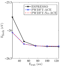
(a) (a)

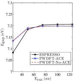
(b) (b)

Figure 1: (color online) (a) Fock exchange energy and (b) HOMO-LUMO gap obtained from Quantum ESPRESSO, PWDFT with and without the ACE formulation for a water molecule.

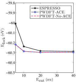
(a) (a)

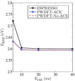
(b) (b)

Figure 2: (color online) (a) Fock exchange energy and (b) HOMO-LUMO gap obtained from Quantum ESPRESSO, PWDFT with and without the ACE formulation for a silicon system with $8$ atoms.

In section 3 the oversampling ratio $r=N_{\varphi}/N_{e}$ is defined. It is conceivable that as $r$ increases, the convergence of the outer iteration for the orbitals $\{\varphi_{i}\}$ can accelerate. Fig. 3 (a) and (b) report the convergence of the difference of the Fock exchange energy at each outer iteration with respect to different oversampling ratio $r$ for the water and silicon system, respectively, as a measure of the convergence of the outer iteration. The kinetic energy cutoff for the water and silicon systems is set to $100$ au and $20$ au, respectively. The convergence without the ACE formulation is also included fir comparison. We observe that as the oversampling ratio increases, the convergence rate of the outer iteration becomes marginally improved. In fact the convergence rate using the ACE formulation with $r=1$ is very close to that without the ACE formulation at all. This indicates that the use of the ACE formulation does not hinder the convergence rate of the hybrid functional calculation.

In order to demonstrate the efficiency of the ACE formulation for hybrid functional calculations, we study three silicon systems with increasing sizes $8$, $64$ and $216$ atoms, respectively. The latter two systems correspond to a silicon unit cell with $8$ atoms replicated into a $2\times 2\times 2$ and a $3\times 3\times 3$ supercell, respectively. Since hybrid functional is implemented in PWDFT so far in the serial mode, we use a relatively small kinetic energy cutoff $E_{\mbox{cut}}=5$ au in these calculations. Nonetheless, the kinetic energy cutoff mainly affects the cost of the FFTs, and we expect that the ACE formulation will become more advantageous with a higher $E_{\mbox{cut}}$ in terms of the reduction of the absolute computational time. Fig. 4 shows the time cost of each SCF iteration for the electron density, which involves $10$ LOBPCG iterations, for the calculation with the HSE functional with and without the ACE formulation. For comparison we also include the time cost of each SCF iteration for the electron density in a GGA functional calculation using the Perdew-Burke-Ernzerhof (PBE) functional ⁷, of which the cost is much less expensive. The cost of the construction phase of the ACE formulation is marked separately as “ACE,Construct” in Fig. 4.

First we confirm that the cost of each hybrid functional calculations is much higher than that of GGA calculations. The time per SCF iteration for the electron density of the HSE calculation without ACE is $42$ times higher than that of the PBE calculation for the $64$ atom system. This ratio becomes $58$ times for the $216$ atom system. With the ACE formulation, this ratio is reduced to $1.18$ and $1.05$, for the $64$ and $216$ atom systems, respectively, i.e. the cost of each HSE calculation in the ACE formulation is only marginally larger than that of the GGA calculation. Although the construction of the ACE still requires solving a large number of Poisson equations, the overall time is greatly reduced since the ACE, once constructed, can be used for multiple SCFs for converging the electron density, until the orbitals $\varphi_{i}$’s are changed in the outer iteration. Even assuming the inner iteration only consists of one SCF iteration, for the system with $216$ atoms, the ACE formulation already achieves a speedup $8.8$ times compared to the standard implementation. The ACE formulation becomes orders of magnitude more efficient when multiple inner SCF iterations is required, which is usually the case both in PWDFT and in other software packages such as Quantum ESPRESSO.

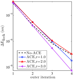
(a) (a) Water molecule

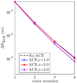
(b) (b) Silicon with $8$ atoms

Figure 3: (color online) Convergence of the difference of the exchange energy.

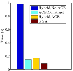
(a) (a)$8$ atoms

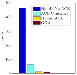
(b) (b)$64$ atoms

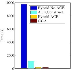
(c) (c)$216$ atoms

Figure 4: (color online) Computational time for silicon systems with increasing system sizes.

5 Conclusion

We have introduced the adaptively compressed exchange operator (ACE) formulation for compressing the Fock exchange operator. The main advantage of the ACE formulation is that there is no loss of accuracy, and its effectiveness does not depend on the size of the band gap. Hence the ACE formulation can be used for insulators, semiconductors as well as metals. We demonstrated the use of the ACE formulation in an iterative framework for solving Hartree-Fock equations and Kohn-Sham equations with hybrid exchange-correlation functionals. The ACE formulation only requires moderate modification of the code, and can potentially be applied to all electronic structure software packages for treating the exchange interaction. The construction cost of the ACE formulation is the same as applying the Fock exchange operator once to the occupied orbitals. Once constructed, the cost of each self-consistent field iteration for the electron density in hybrid functional calculations becomes only marginally larger than that of GGA calculations. Our numerical results indicate that the computational advantage of the ACE formulation can be clearly observed even for small systems with tens of atoms.

For insulating systems, the cost of the ACE formulation can be further reduced when combined with linear scaling type methods. For range separated hybrid functionals, it might even be possible to localize the projection vectors $\xi_{k}$’s due to the screened Coulomb interaction in the real space. This could further reduce the construction as well as the application cost of the ACE, and opens the door to Hartree-Fock-like calculations for a large range of systems beyond reach at present.

This work was partially supported by Laboratory Directed Research and Development (LDRD) funding from Berkeley Lab, provided by the Director, Office of Science, of the U.S. Department of Energy under Contract No. DE-AC02-05CH11231, by the Scientific Discovery through Advanced Computing (SciDAC) program and the Center for Applied Mathematics for Energy Research Applications (CAMERA) funded by U.S. Department of Energy, Office of Science, Advanced Scientific Computing Research and Basic Energy Sciences, and by the Alfred P. Sloan fellowship.

References

- Hohenberg and Kohn 1964 Hohenberg, P.; Kohn, W. Phys. Rev. 1964, 136, B864–B871
- Kohn and Sham 1965 Kohn, W.; Sham, L. Phys. Rev. 1965, 140, A1133–A1138
- Ceperley and Alder 1980 Ceperley, D. M.; Alder, B. J. Phys. Rev. Lett. 1980, 45, 566–569
- Perdew and Zunger 1981 Perdew, J. P.; Zunger, A. Phys. Rev. B 1981, 23, 5048–5079
- Becke 1988 Becke, A. D. Phys. Rev. A 1988, 38, 3098–3100
- Lee et al. 1988 Lee, C.; Yang, W.; Parr, R. G. Phys. Rev. B 1988, 37, 785–789
- Perdew et al. 1996 Perdew, J. P.; Burke, K.; Ernzerhof, M. Phys. Rev. Lett. 1996, 77, 3865–3868
- Staroverov et al. 2003 Staroverov, V. N.; Scuseria, G. E.; Tao, J.; Perdew, J. P. J. Chem. Phys. 2003, 119, 12129–12137
- Zhao and Truhlar 2008 Zhao, Y.; Truhlar, D. G. Theor. Chem. Acc. 2008, 120, 215–241
- Becke 1993 Becke, A. D. J. Chem. Phys. 1993, 98, 5648
- Perdew et al. 1996 Perdew, J. P.; Ernzerhof, M.; Burke, K. J. Chem. Phys. 1996, 105, 9982–9985
- Heyd et al. 2003 Heyd, J.; Scuseria, G. E.; Ernzerhof, M. J. Chem. Phys. 2003, 118, 8207–8215
- Heyd et al. 2006 Heyd, J.; Scuseria, G. E.; Ernzerhof, M. J. Chem. Phys. 2006, 124, 219906
- Goedecker 1999 Goedecker, S. Rev. Mod. Phys. 1999, 71, 1085
- Bowler and Miyazaki 2012 Bowler, D. R.; Miyazaki, T. Rep. Prog. Phys. 2012, 75, 036503
- Kohn 1996 Kohn, W. Phys. Rev. Lett. 1996, 76, 3168–3171
- Prodan and Kohn 2005 Prodan, E.; Kohn, W. Proc. Natl. Acad. Sci. 2005, 102, 11635–11638
- Foster and Boys 1960 Foster, J. M.; Boys, S. F. Rev. Mod. Phys. 1960, 32, 300
- Marzari and Vanderbilt 1997 Marzari, N.; Vanderbilt, D. Phys. Rev. B 1997, 56, 12847
- Marzari et al. 2012 Marzari, N.; Mostofi, A. A.; Yates, J. R.; Souza, I.; Vanderbilt, D. Rev. Mod. Phys. 2012, 84, 1419–1475
- Gygi 2009 Gygi, F. Phys. Rev. Lett. 2009, 102, 166406
- E et al. 2010 E, W.; Li, T.; Lu, J. Proc. Natl. Acad. Sci. 2010, 107, 1273–1278
- Ozoliņš et al. 2013 Ozoliņš, V.; Lai, R.; Caflisch, R.; Osher, S. Proc. Natl. Acad. Sci. 2013, 110, 18368–18373
- Damle et al. 2015 Damle, A.; Lin, L.; Ying, L. J. Chem. Theory Comput. 2015, 11, 1463–1469
- Wu et al. 2009 Wu, X.; Selloni, A.; Car, R. Phys. Rev. B 2009, 79, 085102
- Gygi and Duchemin 2012 Gygi, F.; Duchemin, I. J. Chem. Theory Comput. 2012, 9, 582–587
- Chen et al. 2010 Chen, W.; Wu, X.; Car, R. Phys. Rev. Lett. 2010, 105, 017802
- DiStasio et al. 2014 DiStasio, R. A.; Santra, B.; Li, Z.; Wu, X.; Car, R. J. Chem. Phys. 2014, 141, 084502
- Dawson and Gygi 2015 Dawson, W.; Gygi, F. J. Chem. Theory Comput. 2015, 11, 4655–4663
- Giannozzi et al. 2009 Giannozzi, P.; Baroni, S.; Bonini, N.; Calandra, M.; Car, R.; Cavazzoni, C.; Ceresoli, D.; Chiarotti, G. L.; Cococcioni, M.; Dabo, I. J. Phys.: Condens. Matter 2009, 21, 395502–395520
- Anderson 1965 Anderson, D. G. J. Assoc. Comput. Mach. 1965, 12, 547–560
- Pulay 1980 Pulay, P. Chem. Phys. Lett. 1980, 73, 393–398
- Davidson 1975 Davidson, E. J. Comput. Phys. 1975, 17, 87–94
- Knyazev 2001 Knyazev, A. V. SIAM J. Sci. Comp. 2001, 23, 517–541
- Lin et al. 2012 Lin, L.; Lu, J.; Ying, L.; E, W. J. Comput. Phys. 2012, 231, 2140–2154
- Hu et al. 2015 Hu, W.; Lin, L.; Yang, C. J. Chem. Phys. 2015, 143, 124110
- Hartwigsen et al. 1998 Hartwigsen, C.; Goedecker, S.; Hutter, J. Phys. Rev. B 1998, 58, 3641–3662
- Pask and Sterne 2005 Pask, J. E.; Sterne, P. A. Phys. Rev. B 2005, 71, 113101–113104
- Marques et al. 2012 Marques, M. A. L.; Oliveira, M. J. T.; Burnus, T. Comput. Phys. Commun. 2012, 183, 2272–2281
- Hutter and Curioni 2005 Hutter, J.; Curioni, A. Parallel Comput. 2005, 31, 1–17