Stable and convergent approximation of two-dimensional vector fields on unstructured meshes

Abstract

A new framework is proposed for analyzing staggered-grid finite difference finite volume methods on unstructured meshes. The new framework employs the concept of external approximation of function spaces, and gauge convergence of numerical schemes through the quantities of vorticity and divergence, instead of individual derivatives of the velocity components. The construction of a stable and convergent external approximation of a simple but relevant vector-valued function space is demonstrated, and the new framework is applied to establish the convergence of the MAC scheme for the incompressible Stokes problem on unstructured meshes.

1 Introduction

In simulations of physical systems, it is often advantageous to stagger the vectorial variables with the scalar variables. The resulting schemes are collectively called staggered-grid schemes. A classical example of staggered-grid scheme is the Marker-and-Cell scheme ([1]), also known as the C-grid in the geoscience community ([2]), in which the mass and other related variables are specified at cell centers and the normal velocity components are specified at cell edges. The MAC scheme is widely accepted as the method of choice for incompressible flows ; see [3] for a review. Since its introduction, it has also been argued that the scheme is suitable for flows at all speeds; see the seminal papers by [4] and [5], as well as later developments by [6, 7, 8, 9, 10]. For geophysical flows, the C-grid scheme has been shown to be superior in resolving inertial-gravity dispersive relations; see the seminal paper by [2], and recent expositions on this topic, [11, 12, 13, 14]. In recent years, to take advantage of the growing power of supercomputers, there has been a push to extend the C-grid scheme onto unstructured meshes for complex problems on complex geometric domains. In this regard, we mention the work by [15, 16, 17].

In this work we concern ourselves with the analysis of staggered-grid numerical schemes on unstructured meshes. Staggered-grid schemes are mostly constructed using the finite difference (FD) or finite volume (FV) techniques, and therefore, with regard to analysis, they pose the same challenges that classical FD/FV schemes do, namely the lack of variational formulations and the use of low-order piecewise constant functions. Staggered-grid schemes on unstructured meshes pose an extra challenge: the normal and/or tangential velocity components specified on the edges may not align with the canonical directions of the original vector field. The last two decades have seen quite some efforts on this topic; the theory for the MAC-scheme on structured meshes is fairly complete, at least when classical fluid problems, such as compressible/incompressible Stokes, are concerned. In 1975, roughly 10 years after the MAC scheme was introduced, Girault ([18]) proposed a finite element method on “interlaced” rectangular meshes for the stationary incompressible Navier-Stokes problem; the method reduces to the classical MAC scheme when the boundaries of the domain align with the mesh lines and a special 4-point quadrature rule is used. First-order error estimates were given for both the velocity and the pressure. Through the co-volume approach, Nicolaides and Wu ([19]) derives the a priori error estimates of the MAC scheme on rectangular meshes for the stationary two-dimensional incompressible Navier-Stokes problem. Kanschat ([20]) shows that, on rectangular meshes, the MAC scheme for incompressible flows is algebraically equivalent to the divergence-conforming discontinuous Galerkin method based on the lowest order Raviart-Thomas elements. Eymard et. al. ([21]) perform the stability and convergence analysis of the MAC scheme for the two- and three-dimensional compressible Stokes problem on rectangular meshes. Chénier et. al. ([22]) consider a variational extension of the MAC to the full Navier Stokes equations on semi-regular, non-conforming, and locally refined meshes. E and Liu ([23]) analyze the MAC scheme for the two-dimensional time-dependent Navier-Stokes equations, again, on rectangular meshes. The situation on unstructured meshes is quite different. The only work known to us on this topic is Nicolaides ([24]), who derives the a priori error estimates for the MAC scheme for the incompressible Stokes problem on unstructured meshes. We should point out that Chou ([25]) derives the a priori error estimates for MAC-like schemes for generalized Stokes on triangular meshes. But the schemes are constructed by approximating both of the canonical velocity components with piecewise linear Petrov-Galerkin elements, and thus are different from the type of schemes considered here.

We aim to develop a new theoretical framework for analyzing staggered-grid schemes for a wide range of fluid problems. There are two essential ingredients to this new framework. The first is the concept of external approximation of function spaces, which was proposed by Céa ([26]), and extensively used by Aubin ([27]) and Temam ([28]). This concept has been used recently by several authors to study the convergence of non-staggered finite volume schemes ([29, 30]). Formal definitions will be given in the next section. Briefly speaking, external approximation adds an auxiliary function space $F$ alongside the original function space $V$ and the discrete function space $V_{h}$ (see Figure 1). With the aid of several mappings defined between these function spaces, elements from $V_{h}$, which are often discontinuous, can now be compared with elements from $V$ in the auxiliary space $F$. The second ingredient of our new framework is the use of vorticity and divergence to gauge the convergence of the numerical schemes. This is a direct reflection of the fact that staggered-grid schemes are best at mimicking the vorticity and/or divergence, but not the canonical components of the velocity field, or any of its gradients in the canonical directions.

The framework is general enough to be applicable to different types of staggered-grid schemes (MAC, co-volume, etc.), and potentially to a wide range of fluid problems (compressible/incompressible Stokes, shallow water equations, etc.) The goal of the current article is to present the analysis framework and to apply it to the first case of interest, the classical incompressible Stokes problem. The existence and uniqueness of a discrete solution, and its convergence to the true solution are established.

After we have completed this work, we were made ware that very similar results have been obtained in [31]. But the current work and the cited work differ in the approaches taken. We utilize an external approximation framework for vector fields for the convergence analysis, while [31] rely on a strong reconstruction operator (to reconstruct the velocity field from either the tangential or normal velocity components) and a compactness result. They also prove the convergence for the pressure field for one version of the MAC schemes, which comes as an extra bonus of their approach. The same issue is not discussed in our work, because the pressure field disappear in the variational form for the problem. On the other hand, it appears that the results of [31] only apply to triangular-Delaunay meshes, while ours apply to arbitrarily unstructured staggered grids. Due to these differences, we are comfortable in publishing this work.

The rest of the article is arranged as follows. In Section 2, we recall the definitions of external approximations, and present the framework for constructing and analyzing external approximations of vector fields on unstructured meshes. In Section 3, we apply the framework to analyze the MAC scheme for the incompressible Stokes problem. We finish in Section 4 with some concluding remarks concerning the current work and future plans.

2 Approximation of vector fields

In the study of partial differential equations (PDEs) governing physical systems, such as fluids, various vector-valued function spaces may appear as the natural setting of the problems. These function spaces usually differ in the level of the regularity and boundary behaviors. We let $\Omega$ be a bounded and simply connected domain on the two-dimensional plane with piecewise smooth boundaries, and in this section, we consider the vector-valued function space

$$V=H^{\mathrm{div}}_{0}(\Omega)\cap H^{\mathrm{curl}}(\Omega).$$ (2.1)

Here $H^{\mathrm{div}}_{0}(\Omega)$ is a space of square-integrable vector-valued functions whose divergence is also square-integrable, and whose normal component vanishes on the boundary (see [32] for details). Similarly, $H^{\mathrm{curl}}(\Omega)$ denotes a space of square-integrable vector-valued functions whose curl is also square-integrable. By [32, Proposition 3.1], the space $V$ is algebraically and topologically included in the space $H^{1}(\Omega)$, and in addition, the $H^{1}$-norm of functions from $V$ can be majorized by the $L^{2}$-norms of their divergence and curl. Thus, $V$ is a Hilbert space with norm

$$\|\boldsymbol{u}\|_{V}^{2}=|\mathrm{div}\boldsymbol{u}|_{0}^{2}+|\mathrm{curl}\boldsymbol{u}|_{0}^{2}.$$ (2.2)

In this section we present a discrete approximation to the function space $V$. We choose to work on this function space because it is quite general but still relevant in the study of fluids. The homogeneous boundary condition on the normal velocity component corresponds to no-flux boundary condition, which is desirable for both viscous and inviscid fluids in closed domains. The discrete approximation to this function space appears to be the most general setting where many of the discrete vector field theories can be established, such as the Helmholtz decomposition theorem. These results will be needed in dealing with specific problems, even though the function spaces may differ.

The approximation that we are about to present is stable and convergent. But before we present the discrete approximations, we need to first recall the definitions of approximations of function spaces, and the concepts of stability and convergence.

2.1 Definitions

Here we recall the definitions of external approximations of normed spaces. Detailed expositions on this topic can be found in [33, 26, 27]. Let $V$ be a linear function space with norm $\|\cdot\|$.

Definition 2.1.

An external approximation of a normed space $V$ is a set consisting of

1. a normed space $F$ and an isomorphism $\Pi$ from $V$ into $F$;

2. a family of triplets $\{V_{h},\,\mathcal{P}_{h},\,\mathcal{R}_{h}\}_{h\in\mathcal{H}}$, in which for each $h$, $V_{h}$ is a normed space, $\mathcal{P}_{h}$ a continuous linear mapping of $V_{h}$ into $F$, $\mathcal{R}_{h}$ a (possibly nonlinear) mapping of $V$ into $V_{h}$.

The relations between the normed spaces and the operators in an external approximation are shown in Figure 1.

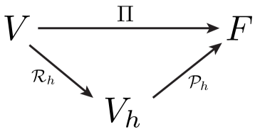
Figure 1: External approximation

The restriction operators may be nonlinear, and, as a consequence, it is not possible to define their norms. The prolongation operator $\mathcal{P}_{h}$ is linear, and its stability and the stability of the external approximation are defined as follows.

Definition 2.2.

The prolongation operators $\mathcal{P}_{h}$ are called stable if their norms

$$\|\mathcal{P}_{h}\|=\sup_{\stackrel{{\scriptstyle u_{h}\in V_{h}}}{{\|u_{h}\|_{h}=1}}}\|\mathcal{P}_{h}u_{h}\|$$

can be majorized independently of $h$. The external approximation of $V$ is sable if the prolongation operators $\mathcal{P}_{h}$ are stable.

Definition 2.3.

An external approximation of a normed space $V$ is convergent if

1. for all $u\in V$,

   $$\lim_{h\rightarrow 0}\mathcal{P}_{h}\mathcal{R}_{h}u=\Pi u$$ (2.3)

   in the strong topology of $F$;

2. a sequence $\mathcal{P}_{h}u_{h}$ converging to some element $\phi$ in the weak topology of $F$ implies that $\phi=\Pi u$ for some $u\in V$.

In practice, it may be difficult to explicitly define the restriction operator $\mathcal{R}_{h}$ for every function in $V$. As it turns out, $\mathcal{R}_{h}$ only needs to be specified for a dense subspace $\mathcal{V}$. If condition (C1) holds for every $\boldsymbol{u}\in\mathcal{V}$, then the definition of $\mathcal{R}_{h}$ can be extended, possibly in nonlinear fashion, to the whole space of $V$ so that the condition holds for all $\boldsymbol{u}\in V$. For a proof, the reader is referred to [33, Section 3.4].

2.2 Specification of the mesh

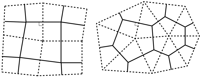
Figure 2: Examples of staggered grid. Left: a quadrilateral staggered grid. Right: a Delaunay-Voronoi staggered grid.

Our approximation of the function space is based on discrete meshes that consist of polygons. To avoid potential technical issues with the boundary, we shall assume that the domain $\Omega$ itself is polygonal. We make use of a pair of staggered meshes, with one called primary and the other called dual. The meshes consist of polygons, called cells, of arbitrary shape, but conforming to the requirements to be specified. The centers of the cells on the primary mesh are the vertices of the cells on the dual mesh, and vice versa. The edges of the primary cells intersect orthogonally with the edges of the dual cells. The line segments of the boundary $\partial\Omega$ pass through the centers of the primary cells that border the boundary. Thus the primary cells on the boundary are only partially contained in the domain. Shown in Figure 2 are two common types of staggered grids: a quadrilateral-quadrilateral staggered grid (left), and a Delaunay-Voronoi tessellation (right).

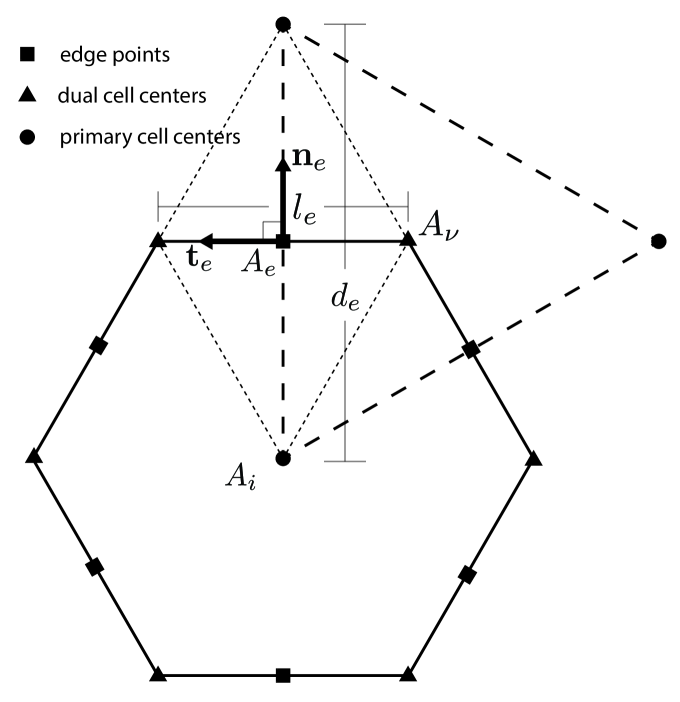
Figure 3: Notations

Table 1: Sets of elements defining the connectivity of an unstructured dual grid.

Set	Definition
EC($i$)	Set of edges defining the boundary of primary cell $A_{i}$
VC($i$)	Set of dual cells that form the vertices primary cell $A_{i}$
CE($e$)	Set of primary cells boarding edge $e$
VE($e$)	Set of dual cells boarding edge $e$
CV($\nu$)	Set of primary cells that form vertices of dual cell $D_{\nu}$
EV($\nu$)	Set of edges that define the boundary of dual cell $D_{\nu}$

In order to construct function spaces on this type of meshes, some notations are in order, for which we follow the conventions made in [16, 17]. As shown in the diagram in Figure 3, the primary cells are denoted as $A_{i},\,1\leq i\leq N_{c}+N_{cb}$, where $N_{c}$ denotes the number of cells that are in the interior of the domain, and $N_{cb}$ the number of cells that are on the boundary. We assume the cells are numbered so that $A_{i}$ with $1\leq i\leq N_{c}$ refer to interior cells. The dual cells, which all lie inside the domain, are denoted as $A_{\nu},\,1\leq\nu\leq N_{v}$. When no confusion should arise, we also use $A_{i}$ and $A_{\nu}$ to denote the areas of the primary cells and dual cells, respectively. Each primary cell edge corresponds to a distinct dual cell edge, and vice versa. Thus the primary and dual cell edges share a common index $e,\,1\leq e\leq N_{e}+N_{eb}$, where $N_{e}$ denotes the number of edge pairs that lie entirely in the interior of the domain, and $N_{eb}$ the number of edge pairs on the boundary, i.e., with dual cell edge aligned with the boundary of the domain. Again, we assume that $1\leq e\leq N_{e}$ refer to interior edges. Upon the edge pair $e$, the distance between the two primary cell centers, which is also the length of the corresponding dual cell edge, is denoted as $d_{e}$, while the distance between the two dual cell centers, which is also the length of the corresponding primary cell edge, is denoted as $l_{e}$. These two edges form the diagonals of a diamond-shaped region, whose vertices consist of the two neighboring primary cell centers and the two neighboring dual centers. The diamond-shaped region is also indexed by $e$, and will be referred to as $A_{e}$. The Euler formula for planar graphs states that the number of primary cell centers $N_{c}+N_{cb}$, the number of vertices (dual cell centers) $N_{v}$, and the number of primary or dual cell edges $N_{e}+N_{eb}$ must satisfy the relation

$$N_{c}+N_{cb}+N_{v}=N_{e}+N_{eb}+1.$$ (2.4)

The connectivity information of the unstructured staggered meshes is provided by six sets of elements defined in Table 1.

For each edge pair, a unit vector $\mathbf{n}_{e}$, normal to the primary cell edge, is specified. A second unit vector $\mathbf{t}_{e}$ is defined as

$$\mathbf{t}_{e}=\mathbf{k}\times\mathbf{n}_{e},$$ (2.5)

with $\mathbf{k}$ standing for the upward unit vector. Thus $\mathbf{t}_{e}$ is orthogonal to the dual cell edge, but tangent to the primary cell edge, and points to the vertex on the left side of $\mathbf{n}_{e}$. For each edge $e$ and for each $i\in\mathrm{CE}(e)$ (the set of cells on edge $e$, see Table 1), we define the direction indicator

$$n_{e,i}=\left\{\begin{aligned} 1&&&\phantom{sssssss}\textrm{if }\mathbf{n}_{e}\textrm{ points away from primary cell }A_{i},\\ -1&&&\phantom{sssssss}\textrm{if }\mathbf{n}_{e}\textrm{ points towards primary cell }A_{i},\\ \end{aligned}\right.$$ (2.6)

and for each $\nu\in\mathrm{VE}(e)$,

$$t_{e,\nu}=\left\{\begin{aligned} 1&&&\phantom{sssssss}\textrm{if }\mathbf{t}_{e}\textrm{ points away from dual cell }A_{\nu},\\ -1&&&\phantom{sssssss}\textrm{if }\mathbf{t}_{e}\textrm{ points towards dual cell }A_{\nu}.\\ \end{aligned}\right.$$ (2.7)

For this study, we make the following regularity assumptions on the meshes. We assume that the diamond-shaped region $A_{e}$ is actually convex. In other words, the intersection point of each edge pair falls inside each of the two edges. We also assume that the meshes are quasi-uniform, in the sense that there exists $h>0$ such that, for each edge $e$,

$$mh\leq l_{e},\,d_{e}\leq Mh$$ (2.8)

for some fixed constants $(m,\,M)$ that are independent of the meshes. The staggered dual meshes are thus designated by $\mathcal{T}_{h}$.

2.3 Discrete scalar fields

For each $1\leq i\leq N_{c}+N_{cb}$, let $\chi_{i}$ be the characteristic function with support on cell $i$, that is,

$$\chi_{i}(x)=\left\{\begin{aligned} &1&\textrm{ if }x\in A_{i},\\ &0&\textrm{ otherwise.}\end{aligned}\right.$$ (2.9)

For each $1\leq\nu\leq N_{v}$, we let $\chi_{\nu}$ be the characteristic function with support on dual cell $\nu$, that is,

$$\chi_{\nu}(x)=\left\{\begin{aligned} &1&\textrm{ if }x\in A_{\nu},\\ &0&\textrm{ otherwise.}\end{aligned}\right.$$ (2.10)

We define $\Phi_{h}$ to be a space of scalar fields associated with the primary mesh,

$$\Phi_{h}=\left\{\varphi_{h}=\sum_{i=1}^{N_{c}+N_{cb}}\varphi_{i}\chi_{i},\textrm{ with }\{\varphi_{i}\}_{i=1}^{N_{c}+N_{cb}}\in\mathbb{R}^{N_{c}+N_{cb}}\right\}.$$ (2.11)

It is a Hilbert space endowed with the discrete $L^{2}$-norm

$$\|\varphi_{h}\|_{\Phi_{h}}^{2}\equiv|\varphi_{h}|_{0}^{2}=\sum_{i=1}^{N_{c}+N_{cb}}A_{i}\varphi_{i}^{2}.$$ (2.12)

We define $\Psi_{h}$ to be a space of scalar fields associated with the dual mesh,

$$\Psi_{h}=\left\{\psi_{h}=\sum_{\nu=1}^{N_{\nu}}\psi_{\nu}\chi_{\nu},\textrm{ with }\{\psi_{\nu}\}_{\nu=1}^{N_{\nu}}\in\mathbb{R}^{N_{\nu}}\right\}.$$ (2.13)

It is a Hilbert space endowed with the discrete $L^{2}$-norm

$$\|\psi_{h}\|_{\Psi_{h}}^{2}\equiv|\psi_{h}|_{0}^{2}=\sum_{\nu=1}^{N_{\nu}}A_{\nu}\psi_{\nu}^{2}.$$ (2.14)

Gradient operators can be defined on scalar fields from $\Phi_{h}$ and $\Psi_{h}$, using the direction indicators $n_{e,i}$ and $t_{e,\nu}$, respectively. On each edge $e$, the discrete gradient operator on $\varphi_{h}\in\Phi_{h}$ is defined as

$$[\nabla_{h}\varphi_{h}]_{e}=\dfrac{-1}{d_{e}}\sum_{i\in\mathrm{CE}(e)}\varphi_{i}n_{e,i},$$ (2.15)

and the skewed discrete gradient operator on $\psi_{h}\in\Psi_{h}$ is defined as

$$[\widetilde{\nabla}_{h}^{\perp}\psi_{h}]_{e}=\dfrac{1}{l_{e}}\sum_{\nu\in\mathrm{VE}(e)}\psi_{\nu}t_{e,\nu}.$$ (2.16)

The situation on the boundary requires some comments. With each boundary edge, only one vertex is associated. Hence on a boundary edge $e$, the definition (2.16) can be written as

$$[\widetilde{\nabla}_{h}^{\perp}\psi_{h}]_{e\textrm{ on boundary}}=\dfrac{1}{l_{e}}\psi_{\nu}t_{e,\nu},$$ (2.17)

where $\nu$ is the single element in $\mathrm{VE}(e)$. This amounts to implicitly requiring that $\psi_{h}$ vanishes on the boundary. We let

$$\nabla_{h}\varphi_{h}=\sum_{e=1}^{N_{e}+N_{eb}}[\nabla_{h}\varphi_{h}]_{e}\chi_{e}\mathbf{n}_{e},$$ (2.18)

$$\widetilde{\nabla}_{h}^{\perp}\psi_{h}=\sum_{e=1}^{N_{e}+N_{eb}}[\widetilde{\nabla}_{h}^{\perp}\psi_{h}]_{e}\chi_{e}\mathbf{n}_{e}.$$ (2.19)

With the gradient operators, semi-$H^{1}$ norms can be defined as well. For $\varphi_{h}\in\Phi_{h}$, and $\psi_{h}\in\Psi_{h}$, we define

$$|\varphi_{h}|_{1,h} \equiv|\nabla_{h}\varphi_{h}|_{0,h},$$ (2.20)

$$|\psi_{h}|_{1,h} \equiv|\widetilde{\nabla}^{\perp}_{h}\psi_{h}|_{0,h}.$$ (2.21)

These semi-$H^{1}$ norms can actually be taken as norms for the corresponding function spaces, thanks to the discrete Poincaré inequalities. We denote by $\dot{\Phi}_{h}$ the subspace of $\Phi_{h}$ that has zero average.

Lemma 2.4 (Discrete Poincaré inequalities for scalar fields).

For $\varphi_{h}\in\dot{\Phi}_{h}$ and $\psi_{h}\in\Psi_{h}$,

$$|\varphi_{h}|_{0,h} \leq C|\varphi_{h}|_{1,h},$$ (2.22)

$$|\psi_{h}|_{0,h} \leq C|\psi_{h}|_{1,h}.$$ (2.23)

In the above, $C$ stands for some generic constants that depend on the domain $\Omega$ only.

The proofs of these inequalities can be found in [34]. The proofs are quite technical, due to the lack of a global Cartesian coordinate system. The main idea is to construct the values of a scalar variable from its discrete derivatives along an arbitrary but fixed direction. The dimension of the domain $\Omega$ along that direction is finite, by assumption. For details, the reader is referred to [34].

2.4 Discrete vector fields

For each $1\leq e\leq N_{e}+N_{eb}$, we let $\chi_{e}$ be the characteristic function with support on the diamond-shaped region $A_{e}$ (see Figure 3, i.e.

$$\chi_{e}(x)=\left\{\begin{aligned} &1&\textrm{ if }x\in A_{e},\\ &0&\textrm{ otherwise.}\end{aligned}\right.$$ (2.24)

We define $V_{h}$ to be a space of discrete vector-fields that equal a constant vector on each $A_{e}$. Specifically,

$$V_{h}=\left\{u_{h}=\sum_{e=1}^{N_{e}+N_{eb}}u_{e}\chi_{e}\mathbf{n}_{e}\right\}.$$ (2.25)

We recall that $\mathbf{n}_{e}$ is a unit vector normal to the primary cell edge $e$.

Around each primary cell $i$, a discrete divergence operator can be defined, per the divergence theorem,

$$\left[\nabla_{h}\cdot u_{h}\right]_{i}=\dfrac{1}{A_{i}}\sum_{e\in\mathrm{EC}(i)}u_{e}l_{e}n_{e,i}.$$ (2.26)

It is worth noting that, on partial cells on the boundary, the summation on the right-hand side only includes fluxes across the edges that are inside the domain and the partial edges that intersect with the boundary, and this amounts to imposing a no-flux condition across the boundary. It is clear from the definition (2.26) that the image of the discrete divergence operator $\nabla_{h}\cdot(\,)$ on each $u_{h}\in V_{h}$ is a scalar field in $\Phi_{h}$,

$$\nabla_{h}\cdot u_{h}=\sum_{i=1}^{N_{c}+N_{cb}}\left[\nabla_{h}\cdot u_{h}\right]_{i}\chi_{i}\quad\in\Phi_{h},$$ (2.27)

and the mapping is linear. Around each dual cell $\nu$, a discrete curl operator can be defined, per Stokes’ theorem,

$$\left[\widetilde{\nabla}_{h}\times u_{h}\right]_{\nu}=\dfrac{-1}{A_{\nu}}\sum_{e\in\mathrm{EV}(\nu)}u_{e}d_{e}t_{e,\nu}.$$ (2.28)

The tilde atop $\nabla$ signifies the involvement of the dual cells. Thus, the image of the discrete curl operator $\widetilde{\nabla}_{h}\times(\,)$ on each $u_{h}\in V_{h}$ is a scalar field in $\Psi_{h}$,

$$\widetilde{\nabla}_{h}\times u_{h}=\sum_{\nu=1}^{N_{v}}\left[\widetilde{\nabla}_{h}\times u_{h}\right]_{\nu}\chi_{\nu}\quad\in\Psi_{h},$$ (2.29)

and the mapping is linear.

$V_{h}$ is a finite dimensional Hilbert space under the discrete $L^{2}$-norm

$$|u_{h}|_{0,h}^{2}\equiv\sum_{e=1}^{N_{e}+N_{eb}}A_{e}u_{e}^{2}.$$ (2.30)

The discrete semi-$H^{1}$-norm on $V_{h}$ is defined as

$$|u_{h}|_{1,h}^{2}\equiv|\nabla_{h}\cdot u_{h}|_{0,h}^{2}+|\widetilde{\nabla}_{h}\times u_{h}|_{0,h}^{2}.$$ (2.31)

$V_{h}$ is a finite dimensional Hilbert space endowed with norm

$$\|u_{h}\|_{V_{h}}^{2}=|u_{h}|_{0,h}^{2}+|u_{h}|_{1,h}^{2}.$$ (2.32)

In fact, the semi-$H^{1}$ norm (2.31) can also be taken as the norm for $V_{h}$, thanks to a Poincaré-type inequality, which will be presented after we state and prove a few basic properties for the discrete divergence and curl operators.

Given the definitions of the norm (2.31) for $V_{h}$ and the norms (2.12) and (2.14) for $\Phi_{h}$ and $\Psi_{h}$, respectively, it is clear that the the discrete divergence operator and the discrete curl operator

$$\nabla_{h}\cdot(\,):\, V_{h}\xrightarrow{\hskip 42.67912pt}\Phi_{h},$$ (2.33)

$$\widetilde{\nabla}_{h}\times(\,):\, V_{h}\xrightarrow{\hskip 42.67912pt}\Psi_{h},$$ (2.34)

are bounded linear operators. From the definitions (2.18) and (2.19), it is clear that $\nabla_{h}(\,)$ and $\widetilde{\nabla}^{\perp}_{h}(\,)$ are linear operators from $\Phi_{h}$ and $\Psi_{h}$, respectively, into $V_{h}$, that is,

$$\nabla_{h}(\,):\, \Phi_{h}\xrightarrow{\hskip 42.67912pt}V_{h},$$ (2.35)

$$\widetilde{\nabla}_{h}^{\perp}(\,):\, \Psi_{h}\xrightarrow{\hskip 42.67912pt}V_{h}.$$ (2.36)

They can be viewed as the “adjoint operators” of the discrete divergence operator and the discrete curl operator, respectively, thanks to the following discrete integration-by-parts formulae.

Lemma 2.5.

For $u_{h}\in V_{h}$, $\varphi_{h}\in\Phi_{h}$, and $\psi_{h}\in\Psi_{h}$, the following relations hold,

$$\left(u_{h},\,\nabla_{h}\varphi_{h}\right)_{0,h} =-\dfrac{1}{2}\left(\nabla_{h}\cdot u_{h},\,\varphi_{h}\right)_{0,h},$$ (2.37)

$$\left(u_{h},\,\widetilde{\nabla}_{h}^{\perp}\psi_{h}\right)_{0,h} =-\dfrac{1}{2}\left(\widetilde{\nabla}_{h}\times u_{h},\,\psi_{h}\right)_{0,h}.$$ (2.38)

Proof.

We verify equation (2.37) first. For arbitrary $u_{h}\in V_{h}$, and $\varphi_{h}\in\Phi_{h}$, by the definitions of the inner products and the discrete operators, we have

$$\left(u_{h},\,\nabla_{h}\varphi_{h}\right)_{0,h} =\sum_{e=1}^{N_{e}+N_{eb}}\sum_{i\in\mathrm{CE}(e)}\dfrac{-A_{e}}{d_{e}}u_{e}\varphi_{i}n_{e,i}$$

$$=\sum_{e=1}^{N_{e}+N_{eb}}\sum_{i\in\mathrm{CE}(e)}-\dfrac{1}{2}l_{e}u_{e}\varphi_{i}n_{e,i}.$$

We now switch the order of summations,

$$\left(u_{h},\,\nabla_{h}\varphi_{h}\right)_{0,h} =-\dfrac{1}{2}\sum_{i=1}^{N_{c}+N_{cb}}\varphi_{i}\sum_{e\in\mathrm{EC}(i)}u_{e}l_{e}n_{e,i}$$

$$=-\dfrac{1}{2}\sum_{i=1}^{N_{c}+N_{cb}}A_{i}\varphi_{i}\left(\dfrac{1}{A_{i}}\sum_{e\in\mathrm{EC}(i)}u_{e}l_{e}n_{e,i}\right).$$

From the definition of the discrete divergence operator (2.27) it follows that

$$\left(u_{h},\,\nabla_{h}\varphi_{h}\right)_{0,h}=-\dfrac{1}{2}\left(\nabla_{h}\cdot u_{h},\,\varphi_{h}\right)_{0,h}.$$

To show (2.38), we again invoke the definitions of the inner product and the discrete operator, and by simple calculations, we find that

$$\left(u_{h},\,\widetilde{\nabla}^{\perp}\psi_{h}\right)_{0,h} =\sum_{e=1}^{N_{e}+N_{eb}}A_{e}u_{e}\left(\dfrac{1}{l_{e}}\sum_{\nu\in\mathrm{VE}(e)}\psi_{\nu}t_{e,\nu}\right)$$

$$=\sum_{e=1}^{N_{e}+N_{eb}}\dfrac{1}{2}u_{e}d_{e}\sum_{\nu\in\mathrm{VE}(e)}\psi_{\nu}t_{e,\nu}$$

$$=\dfrac{1}{2}\sum_{e=1}^{N_{e}+N_{eb}}u_{e}d_{e}\sum_{\nu\in VE(e)}\psi_{\nu}t_{e,\nu}.$$

Now we switch the order of summations,

$$\left(u_{h},\,\widetilde{\nabla}^{\perp}\psi_{h}\right)_{0,h} =\dfrac{1}{2}\sum_{\nu=1}^{N_{\nu}}\psi_{\nu}\sum_{e\in\mathrm{EV}(\nu)}u_{e}d_{e}t_{e,\nu}$$

$$=-\dfrac{1}{2}\sum_{\nu=1}^{N_{\nu}}A_{\nu}\psi_{\nu}\left(\dfrac{-1}{A_{\nu}}\sum_{e\in\mathrm{EV}(\nu)}u_{e}d_{e}t_{e,\nu}\right).$$

From the definition of the discrete curl operator (2.29) on the dual mesh, it follows that

$$\left(u_{h},\,\widetilde{\nabla}_{h}^{\perp}\psi_{h}\right)_{0,h}=-\dfrac{1}{2}\left(\widetilde{\nabla}_{h}\times u_{h},\,\psi_{h}\right)_{0,h}.$$

∎

It is clear that equations (2.37) and (2.38) are, respectively, the discrete versions of the integration-by-parts formulae

$$\int_{\Omega}\boldsymbol{u}\cdot\nabla\varphi dx= -\int_{\Omega}\nabla\cdot\boldsymbol{u}\varphi dx, \forall\boldsymbol{u}\in H^{\mathrm{div}}_{0}(\Omega),\,\varphi\in H^{1}(\Omega),$$ (2.39)

$$\int_{\Omega}\boldsymbol{u}\cdot\nabla^{\perp}\psi dx= -\int_{\Omega}\nabla\times\boldsymbol{u}\psi dx, \forall\boldsymbol{u}\in H^{\mathrm{curl}}(\Omega),\,\psi\in H^{1}_{0}(\Omega).$$ (2.40)

The factor of one half in the discrete version stems from the fact that the discrete vector fields $u_{h}$, $\nabla_{h}\varphi_{h}$, and $\widetilde{\nabla}^{\perp}\psi_{h}$ contain only the normal component (in the direction of $\mathbf{n}_{e}$). The no-flux boundary condition, required for (2.39), is implied in the specification of the discrete divergence operator, and the homogeneous boundary condition on the scalar field $\psi$, required for (2.40), is implied in the specification of the discrete skewed gradient operator $\widetilde{\nabla}^{\perp}$ on $\psi_{h}$. See the comments following definition (2.26) and the comments following (2.17). It is worth pointing out that the identity (2.38) is still valid if $u_{h}$ vanishes on the boundary and $\psi_{h}$ is arbitrary. Indeed, we will encounter this situation in the next section in dealing with the incompressible Stokes problem.

In two-dimension, it is well known that a non-divergent vector field is the curl of a scalar field, and an irrotational vector field is the gradient of a scalar field, and the set of non-divergent vector functions and the set of irrotational vector functions form an orthogonal decomposition of the $L^{2}(\Omega)\times L^{2}(\Omega)$ function space ([32, Section 3]). We now establish the discrete version of these results for the space $V_{h}$.

Lemma 2.6.

Assume that the domain $\Omega$ is simply connected. For $u_{h}\in V_{h}$,

$$\nabla_{h}\cdot u_{h}=0$$ (2.41)

if and only if there exists $\psi_{h}\in\Psi_{h}$ such that

$$u_{h}=\widetilde{\nabla}_{h}^{\perp}\psi_{h}.$$ (2.42)

Proof.

We first show sufficiency. Let $u_{h}$ be given by a scalar field $\psi_{h}\in\Psi_{h}$ via

$$u_{h}=\widetilde{\nabla}^{\perp}_{h}\psi_{h}.$$

Then for an arbitrary cell $i$,

$$[\nabla_{h}\cdot u_{h}]_{i}= \dfrac{1}{A_{i}}\sum_{e\in\mathrm{EC}(i)}u_{e}l_{e}n_{e,i}$$

$$= \dfrac{1}{A_{i}}\sum_{e\in\mathrm{EC}(i)}\left(\dfrac{1}{l_{e}}\sum_{\nu\in\mathrm{VE}(e)}\psi_{\nu}t_{e,\nu}\right)l_{e}n_{e,i}$$

$$= \dfrac{1}{A_{i}}\sum_{e\in\mathrm{EC}(i)}\sum_{\nu\in\mathrm{VE}(e)}\psi_{\nu}t_{e,\nu}n_{e,i}.$$

It is easy to verify that, surrounding cell $i$, each $\psi_{\nu}$ appears exactly twice, with opposite signs. Hence the summation is zero, and (2.41) is proven.

For necessity, let $u_{h}\in V_{h}$ be a discrete vector field such that (2.41) holds. For an arbitrary vertex, say $\nu=1$, we set $\psi_{\nu}=0$, or any other constants. For a vertex $\nu$ that is connected to vertex $1$ by a common edge, $\psi_{\nu}$ can be obtained by integrating $u_{e}$ on the common edge. Specifically, $\psi_{\nu}$ on neighboring vertices can be obtained through the relation

$$u_{e}l_{e}=\sum_{\nu\in\mathrm{VE}(e)}\psi_{\nu}t_{e,\nu}.$$ (2.43)

It is obvious that, on edges that originate from vertex $1$, $u_{h}$ is given by the formula (2.42).

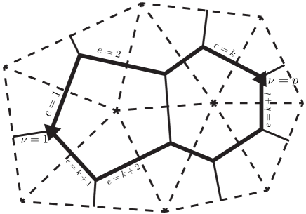
Figure 4: Closed path around primary cells

The integration can be further carried out to reach points that are not directly connected to vertex $1$. By assumption, the domain $\Omega$ is connected, and therefore every $\psi_{\nu}$ can be determined this way. Since two arbitrarily given vertices can be connected by multiple paths, we need to verify that results obtained over different paths are consistent. To this end, we suppose that vertex $p$ is connected to vertex 1 through two paths, the first consisting of edges $1$, $2$, $\cdots$, $k$, and the second consisting of edges $k+1$, $k+2$, $\cdots$, $k+l$. We also suppose that the integration along the first path yields $\psi_{p}$, and the integration along the second path yields $\widetilde{\psi}_{p}$. We shall show that these two results are identical. We note that the two paths form a closed curve, and the surrounded region consists of primary cells, and no holes (Figure 4). By the assumption (2.41), the net flux across the boundary of each individual cell is zero, and therefore, it must also be zero across the boundary of the surrounded region, that is,

$$\sum_{e=1}^{k+l}u_{e}l_{e}n_{e}=0,$$ (2.44)

where $n_{e}$ is an indicator of the direction of the unit normal vector $\mathbf{n}_{e}$ with respect of the surrounded region, and it is defined as

$$n_{e}=\left\{\begin{aligned} &1&&\textrm{if $\mathbf{n}_{e}$ points outward,}\\ &-1&&\textrm{if $\mathbf{n}_{e}$ points inward.}\end{aligned}\right.$$

Multiplying (2.43) by $n_{e}$ and summing over $1\leq e\leq k$, we have

$$\sum_{e=1}^{k}u_{e}l_{e}n_{e}=\sum_{e=1}^{k}\sum_{e=1}^{k}\sum_{\nu\in\mathrm{VE}(e)}\psi_{\nu}t_{e,mu}n_{e}.$$

On the right-hand side, each $\psi_{\nu}$ except $\psi_{1}$ and $\psi_{\partial}$ appears exactly twice, but with opposite signs. Hence

$$\sum_{e=1}^{k}u_{e}l_{e}n_{e}=-\psi_{1}+\psi_{p}.$$

Similarly, along the second path, we have

$$\sum_{e=k+1}^{k+l}u_{e}l_{e}n_{e}=\psi_{1}-\widetilde{\psi}_{p}.$$

It follows from (2.44) that

$$\psi_{p}=\widetilde{\psi}_{p}.$$

∎

Lemma 2.7.

Assume that the domain $\Omega$ is simply connected. For $u_{h}\in V_{h}$,

$$\widetilde{\nabla}_{h}\times u_{h}=0$$ (2.45)

if and only if there exists $\varphi_{h}\in\Phi_{h}$ such that

$$u_{h}=\nabla_{h}\varphi_{h}.$$ (2.46)

Proof.

We first verify the sufficiency. We let $\varphi_{h}\in\Phi_{h}$ such that

$$u_{h}=\nabla_{h}\varphi_{h}.$$

Then for an arbitrary vertex $\nu$,

$$[\widetilde{\nabla}\times u_{h}]_{\nu} =\dfrac{-1}{A_{\nu}}\sum_{e\in\mathrm{EV}(\nu)}u_{e}d_{e}t_{e,\nu}$$

$$=\dfrac{-1}{A_{\nu}}\sum_{e\in\mathrm{EV}(\nu)}\dfrac{-1}{d_{e}}\left(\sum_{i\in\mathrm{CE}(e)}\varphi_{i}n_{e,i}\right)d_{e}t_{e,\nu}$$

$$=\dfrac{1}{A_{\nu}}\sum_{e\in EV(\nu)}\sum_{i\in\mathrm{CE}(e)}\varphi_{i}n_{e,i}t_{e,\nu}.$$

We note that in the expression above concerning an arbitrary vertex $\nu$, each $\varphi_{i}$ appears exactly twice, but with opposite signs. Hence the summation vanishes for each $\nu$.

For necessity, we assume that $u_{h}\in V_{h}$, and (2.45) holds. We pick an arbitrary cell center, say cell $1$, and set

$$\varphi_{1}=0.$$

Then we determine the values of the $\varphi$ at neighboring cell centers by integrating $u_{e}$ along the dual cell edges. Specifically, $\varphi_{i}$ at a neighboring cell center is obtained via

$$u_{e}d_{e}=-\sum_{i\in\mathrm{CE}(e)}\varphi_{i}n_{e,i}.$$ (2.47)

It is clear that the relation (2.46) holds along dual cell edges originating from cell $1$.

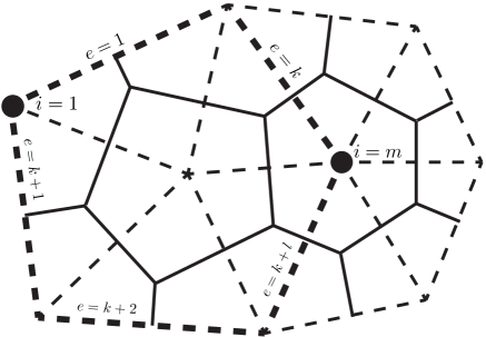
Figure 5: Two paths around dual cells

The integration is then carried out to define $\varphi_{i}$’s at cell centers not directly connected to cell $1$. The domain is connected, and therefore each $\varphi_{i}$ can be defined this way. To ensure that a discrete scalar field $\varphi_{h}$ is well-defined, we just need to show that, for an arbitrary cell $m$, integrations along any two paths yield the same value. Without loss of generality, we assume that the first path consists of dual cell edges $1$, $2$, $\cdots$, $k$ (Figure 5), and the integration yields $\varphi_{m}$, and the second path consists of dual cell edges $k+1$, $k+2$, $\cdots$, $k+l$, and the integration yields $\widetilde{\varphi}_{m}$. These two paths form a closed curve, and the enclosed region is made up of dual cells, and no holes. By the assumption (2.45), the circulation around each dual cell is zero, and therefore the circulation around the entire enclosed region is also zero, that is,

$$\sum_{e=1}^{k+l}u_{e}d_{e}t_{e}=0,$$ (2.48)

where $t_{e}$ is an indicator of the direction of the unit tangent vector $\mathbf{t}_{e}$ with respect to the enclosed region,

$$t_{e}=\left\{\begin{aligned} &1&&\textrm{if $\mathbf{t}_{e}$ points outward,}\\ &-1&&\textrm{if $\mathbf{t}_{e}$ points inward.}\end{aligned}\right.$$

Multiplying (2.47) by $t_{e}$ and summing over $1\leq e\leq k$, we obtain

$$\sum_{e=1}^{k}u_{e}d_{e}t_{e}=-\sum_{e=1}^{k}\sum_{i\in\mathrm{CE}(e)}\varphi_{i}n_{e,i}t_{e}.$$

On the right-hand side, each $\varphi_{i}$ except $\varphi_{1}$ and $\varphi_{m}$ appears exactly twice but with opposite signs, and hence

$$\sum_{e=1}^{k}u_{e}d_{e}t_{e}=-\varphi_{1}+\varphi_{m}.$$

Similarly, multiplying (2.47) by $t_{e}$ and summing over $k+1\leq e\leq k+l$, we find

$$\sum_{e=1}^{k}u_{e}d_{e}t_{e}=\varphi_{1}-\widetilde{\varphi}_{m}.$$

In view of (2.48), we conclude that

$$\varphi_{m}=\widetilde{\varphi}_{m}.$$

∎

Lemma 2.8.

The space of discrete vector fields has the following orthogonal decomposition

$$V_{h}=\{u_{h}\in V_{h}|\,\nabla_{h}\cdot u_{h}=0\}\oplus\{u_{h}\in V_{h}|\,\widetilde{\nabla}\times u_{h}=0\}.$$ (2.49)

Proof.

We first show that the two sets are orthogonal. We let $u_{h},\,u^{\#}_{h}\in V_{h}$ such that $\nabla\cdot u_{h}=0$ and $\widetilde{\nabla}\times u^{\#}_{h}=0$. Then by Lemma 2.6, there exists $\psi_{h}\in\Psi_{h}$ such that $u_{h}=\widetilde{\nabla}^{\perp}\psi_{h}$. Using the integration by parts formula (2.38), we find that

$$(u_{h},\,u^{\#}_{h})=(\widetilde{\nabla}^{\perp}\psi_{h},\,u^{\#}_{h})=-\dfrac{1}{2}(\psi_{h},\,\widetilde{\nabla}\times u^{\#}_{h})=0.$$

Thus $u_{h}$ and $u^{\#}_{h}$ are orthogonal.

We now show that each element of $V_{h}$ is the sum of an non-divergent discrete vector field and an irrotational discrete vector field. In view of Lemmas 2.6 and 2.7, this amounts to saying that there exist $\varphi_{h}\in\Phi_{h}$ and $\psi_{h}\in\Psi_{h}$ such that

$$u_{h}=\widetilde{\nabla}^{\perp}\psi_{h}+\nabla_{h}\varphi_{h}.$$ (2.50)

This single equation actually represents a system of equations involving the normal velocity components $u_{e}$, $1\leq e\leq N_{e}+N_{eb}$, on the edges, and the discrete scalar variable $\varphi_{i}$, $1\leq i\leq N_{c}+N_{cb}$, at cell centers, and $\psi_{\nu}$, $1\leq\nu\leq N_{v}$, at cell vertices. There are $N_{c}+N_{cb}+N_{v}$ unknowns. The system reads

$$[\widetilde{\nabla}^{\perp}\psi_{h}]_{e}+[\nabla_{h}\varphi_{h}]_{e}=u_{e},\qquad 1\leq e\leq N_{e}+N_{eb}.$$ (2.51)

Hence there are $N_{e}+N_{eb}$ equations. By Euler’s formula (2.4) there is one more unknown than the number of equations. This reflects the fact that any $\varphi_{h}$ that satisfies (2.50) will still satisfy the equation after an addition of any constant. To make the solution unique, we can impose an extra constraint requiring that the area weighted average of $\varphi_{h}$ be zero, that is,

$$\int_{\Omega}\varphi_{h}dx=0,\quad\textrm{or equivalently, }\quad\sum_{i=1}^{N_{c}+N_{cb}}A_{i}\varphi_{i}=0.$$ (2.52)

Equations (2.51) and (2.52) form a square linear system. To show that this system has a unique solution for an arbitrary $u_{h}\in V_{h}$, we only need to show that the homogeneous system

$$\left\{\begin{aligned} &[\widetilde{\nabla}^{\perp}\psi_{h}]_{e}+[\nabla_{h}\varphi_{h}]_{e}=0,\qquad 1\leq e\leq N_{e}+N_{eb},\\ &\sum_{i=1}^{N_{c}+N_{cb}}A_{i}\varphi_{i}=0,\end{aligned}\right.$$ (2.53)

or equivalently,

$$\left\{\begin{aligned} &\widetilde{\nabla}^{\perp}\psi_{h}+\nabla_{h}\varphi_{h}=0,\\ &\int_{\Omega}\varphi_{h}dx=0,\end{aligned}\right.$$ (2.54)

has only trivial solutions. It is clear that $\varphi_{h}=0$ and $\psi_{h}=0$ are solutions to the system (2.54). We let $\varphi_{h}$ and $\psi_{h}$ be arbitrary discrete scalar functions that also satisfy the system. Applying the discrete curl operator $\widetilde{\nabla}_{h}\times(\,)$ to the first equation of (2.54), we obtain

$$\widetilde{\nabla}_{h}\times\widetilde{\nabla}^{\perp}\psi_{h}=0.$$ (2.55)

Multiplying (2.55) by $\psi_{h}$, and integrating by parts using (2.38), we find that

$$\left(\widetilde{\nabla}^{\perp}\psi_{h},\,\widetilde{\nabla}^{\perp}\psi_{h}\right)=0.$$ (2.56)

Hence

$$\widetilde{\nabla}^{\perp}\psi_{h}=0,\quad\textrm{or equivalently, }[\widetilde{\nabla}^{\perp}\psi_{h}]_{e}=0,\,\forall 1\leq e\leq N_{e}+N_{eb}.$$ (2.57)

Noticing the definition (2.17) of the skewed discrete gradient operator $\widetilde{\nabla}^{\perp}$ on the boundary, we conclude that

$$\psi_{h}=0\qquad\textrm{(i.e.~{}{}}\psi_{\nu}=0\quad\forall 1\leq\nu\leq N_{v}).$$ (2.58)

Applying the discrete divergence operator $\nabla\cdot(\,)$ to the first equation of (2.54) again, we obtain

$$\nabla_{h}\cdot(\nabla_{h}\varphi_{h})=0.$$ (2.59)

Multiplying (2.59) by $\varphi_{h}$ and integrating by parts using (2.37), we find that

$$\left(\nabla_{h}\varphi_{h},\,\nabla_{h}\varphi_{h}\right)=0.$$ (2.60)

Hence

$$\nabla_{h}\varphi_{h}=0.$$ (2.61)

Under the constraint $\eqref{eq:70}_{2}$, $\varphi_{h}$ must vanish everywhere, that is,

$$\varphi_{h}=0\qquad\textrm{(i.e.~{}{}}\varphi_{i}=0\quad\forall 1\leq i\leq N_{c}+N_{cb}).$$ (2.62)

∎

A discrete Poincaré inequality concerning the $L^{2}$-norm (2.30) and the semi-$H^{1}$ norm (2.31) of $V_{h}$ can be established, which allows us to use the semi-$H^{1}$ norm as the norm for $V_{h}$.

Lemma 2.9 (Discrete Poincaré inequality for vector fields).

For $u_{h}\in V_{h}$,

$$|u_{h}|_{0,h}\leq C|u_{h}|_{1,h}.$$ (2.63)

Proof.

By Lemma 2.8, there exist unique $\psi_{h}\in\Psi_{h}$ $\varphi_{h}\in\dot{\Phi}_{h}$ such that

$$u_{h}=\widetilde{\nabla}_{h}^{\perp}\psi_{h}+\nabla_{h}\varphi_{h}.$$ (2.64)

It is easy to see that $\psi_{h}$ and $\varphi_{h}$ satisfy the discrete elliptic equations

$$\widetilde{\nabla}_{h}\times\widetilde{\nabla}_{h}^{\perp}\psi_{h} =\widetilde{\nabla}_{h}\times u_{h},$$ (2.65)

$$\nabla_{h}\cdot\nabla_{h}\varphi_{h} =\nabla_{h}\cdot u_{h}.$$ (2.66)

With the aid of the integration by parts formulae (2.37) and (2.38), and the discrete Poincaré inequalities (2.22) and (2.23) for scalar fields, we derive the discrete analogues to the classical energy bounds for elliptic problems,

$$|\varphi_{h}|_{0,h}\leq C|\varphi_{h}|_{1,h}\leq C|\nabla_{h}\cdot u_{h}|_{0,h},$$ (2.67)

$$|\psi_{h}|_{0,h}\leq C|\psi_{h}|_{1,h}\leq C|\widetilde{\nabla}_{h}\times u_{h}|_{0,h}.$$ (2.68)

Here, $C$ stands for some generic constants that depend neither on the function nor the mesh resolution $h$. Then, by the orthogonal decomposition (2.64), and the estimates just obtained on $\varphi_{h}$ and $\psi_{h}$,

$$|u_{h}|_{0,h}^{2} =|\widetilde{\nabla}^{\perp}_{h}\psi_{h}|_{0,h}^{2}+|\nabla_{h}\varphi_{h}|_{0,h}^{2}$$

$$=|\psi_{h}|_{1,h}^{2}+|\varphi_{h}|_{1,h}^{2}$$

$$\leq C\left(|\widetilde{\nabla}_{h}\times u_{h}|_{0,h}^{2}+|\nabla_{h}\cdot u_{h}|_{0,h}^{2}\right)$$

$$=C|u_{h}|_{1,h}^{2}.$$

The claim is thus proven. ∎

2.5 External approximation of $V$

We recall that

$$V=H^{1}(\Omega)\cap H^{\mathrm{div}}_{0}(\Omega).$$

We let $F=H\equiv L^{2}(\Omega)\times L^{2}(\Omega)$, and for each $\boldsymbol{u}\in V$, we define

$$\Pi\boldsymbol{u}=(\nabla\times\boldsymbol{u},\,\nabla\cdot\boldsymbol{u})\quad\in F.$$ (2.69)

It is clear that, thanks to the equality (2.2),

$$\Pi:\,V\xrightarrow{\hskip 42.67912pt}F$$ (2.70)

is an isomorphism. For each $u_{h}\in V_{h}$, we define

$$\mathcal{P}_{h}u_{h}=(\widetilde{\nabla}_{h}\times u_{h},\,\nabla_{h}\cdot u_{h})\quad\in\Psi_{h}\times\Phi_{h}\subset F.$$ (2.71)

Clearly $\mathcal{P}_{h}$ is a bounded linear operator from $V_{h}$ into $F$. We now define the restriction operator $\mathcal{R}_{h}$. We only need to define $\mathcal{R}_{h}$ on a dense subspace of $V$ ([33]). We let

$$\mathcal{V}=\{\boldsymbol{u}\in C^{\infty}(\overline{\Omega}),\boldsymbol{u}\cdot\mathbf{n}=0\textrm{ on }\partial\Omega\}.$$ (2.72)

Clearly $\mathcal{V}$ is a dense subspace of $V$. For each $\boldsymbol{u}\in\mathcal{V}$, we let $(\omega,\,\delta)=\Pi\boldsymbol{u}$. We then define their associated discrete scalar fields by

$$\omega_{h}=\sum_{\nu=1}^{N_{v}}\omega_{\nu}\chi_{\nu}\quad\in\Psi_{h},$$ (2.73)

$$\delta_{h}=\sum_{i=1}^{N_{c}+N_{cb}}\delta_{i}\chi_{\nu}\quad\in\Psi_{h}.$$ (2.74)

In the above, the discrete variables $\delta_{i}$ is set to be the average of $\delta$ on primary cell $A_{i}$, i.e.

$$\delta_{i}=\dfrac{1}{|A_{i}|}\int_{A_{i}}\delta dx,$$ (2.75)

so that, by the divergence theorem,

$$\int_{\Omega}\delta_{h}dx=\int_{\Omega}\delta dx=\int_{\partial\Omega}\boldsymbol{u}\cdot\mathbf{n}ds=0.$$ (2.76)

The discrete variables $\omega_{\nu}$ can be specified in various ways, depending on the problem. For example, $\omega_{\nu}$ can be defined in the same way that $\delta_{i}$ is defined, or it can simply be the value of $\omega$ at the center of the dual cell $A_{\nu}$,

$$\omega_{\nu}=\omega(x_{\nu}),$$ (2.77)

with $x_{\nu}$ being the coordinates of the dual cell center. Then we let $u_{h}\in V_{h}$ be the discrete vector field from that satisfy

$$\left\{\begin{aligned} &\widetilde{\nabla}_{h}\times u_{h}=\omega_{h},\\ &\nabla_{h}\cdot u_{h}=\delta_{h}.\end{aligned}\right.$$ (2.78)

Assuming that the system (2.78) is well-posed, i.e. it has a unique solution, we define such $u_{h}$ to be the image of $\mathcal{R}_{h}$ on $\boldsymbol{u}$,

$$\mathcal{R}_{h}\boldsymbol{u}=u_{h}.$$ (2.79)

We now show the well-posedness of the problem (2.78).

Lemma 2.10.

For any $(\omega_{h},\,\delta_{h})\in\Psi_{h}\times\Phi_{h}$ satisfying $\int_{\Omega}\delta_{h}dx=0$, the problem (2.78) has a unique solution $u_{h}\in V_{h}$.

Proof.

We rewrite the system (2.78) in terms of the discrete variables associated with the cell centers, cell vertices, and cell edges,

$$\left\{\begin{aligned} &\dfrac{-1}{A_{\nu}}\sum_{e\in\mathrm{EV}(\nu)}u_{e}d_{e}t_{e,\nu}=\omega_{\nu},&&1\leq\nu\leq N_{v},\\ &\dfrac{1}{A_{i}}\sum_{e\in\mathrm{EC}(i)}u_{e}l_{e}n_{e,i}=\delta_{i},&&1\leq i\leq N_{c}+N_{cb}.\end{aligned}\right.$$ (2.80)

It is clear that there are $N_{e}+N_{eb}$ unknowns, and $N_{v}+N_{c}+N_{cb}$ equations. According to the Euler formula (2.4), there is one more equation than the number of unknowns. Hence the data on the right-hand side of (2.80) need to satisfy some constraint so that they may belong to the range of the linear operator associated with the system on the left-hand side. This constraint is provided by the assumption $\int_{\Omega}\delta_{h}dx=0$, because the integral of the left-hand side of the second equation in $~{}\eqref{eq:79}$ always vanishes. Hence for arbitrary $(\omega_{h},\,\delta_{h})\in\Psi_{h}\times\Phi_{h}$ satisfying the constraint, the system (2.80) or (2.78) has a unique solution if and only if the homogeneous system

$$\left\{\begin{aligned} &\widetilde{\nabla}_{h}\times u_{h}=0,\\ &\nabla_{h}\cdot u_{h}=0,\end{aligned}\right.$$ (2.81)

has only trivial solutions, which is evident from Lemma 2.8. ∎

Lemma 2.11.

The external approximation that comprises of the function space $F$, the isomorphic mapping $\Pi$, and the family of triplets $(V_{h},\,\mathcal{R}_{h},\,\mathcal{P}_{h})_{h\in\mathcal{H}}$ is a stable and convergent approximation of $V$.

Proof.

By Definition 2.2, the external approximation is stable because the prolongation operator is stable.

For convergence, we need to verify the two conditions specified in Definition 2.3. We only need to verify (2.3) for $\boldsymbol{u}\in\mathcal{V}$ (see (2.72)). For an arbitrary $\boldsymbol{u}\in\mathcal{V}$, we let $(\omega,\delta)=\Pi\boldsymbol{u}$, and, for each $1\leq\nu\leq N_{v}$ and $1\leq i\leq N_{c}+N_{cb}$,

$$\omega_{\nu}=\overline{\omega}^{A_{\nu}},\qquad\delta_{i}=\overline{\delta}^{A_{i}}.$$

Then by the definition (2.79) of the restriction operator $\mathcal{R}_{h}$ and the definition (2.71) of the prolongation operator $\mathcal{P}_{h}$,

$$\mathcal{P}_{h}\mathcal{R}_{h}\boldsymbol{u}=\left(\sum_{\nu=1}^{N_{v}}\omega_{\nu}\chi_{\nu},\,\sum_{i=1}^{N_{c}+N_{cb}}\delta_{i}\chi_{i}\right),$$

and

$$\|\mathcal{P}_{h}\mathcal{R}_{h}\boldsymbol{u}-\Pi\boldsymbol{u}\|_{F}^{2}= \int_{\Omega}\left(\sum_{\nu=1}^{N_{v}}\omega_{\nu}\chi_{\nu}-\omega\right)^{2}dx+\int_{\Omega}\left(\sum_{i=1}^{N_{c}+N_{cb}}\delta_{i}\chi_{i}-\delta\right)^{2}dx$$

$$= \sum_{\nu=1}^{N_{v}}\int_{A_{\nu}}(\omega_{\nu}-\omega)^{2}dx+\sum_{i=1}^{N_{c}+N_{cb}}\int_{A_{i}}(\delta_{i}-\delta)^{2}dx$$

$$\leq \left(|\nabla\omega|^{2}_{\infty}+|\nabla\delta|^{2}_{\infty}\right)\left(\sum_{\nu=1}^{N_{v}}\int_{A_{\nu}}1dx+\sum_{i=1}^{N_{c}+N_{cb}}\int_{A_{i}}1dx\right)h^{2}$$

$$\leq 2|\Omega|\left(|\nabla\omega|^{2}_{\infty}+|\nabla\delta|^{2}_{\infty}\right)h^{2}.$$

Therefore $\|\mathcal{P}_{h}\mathcal{R}_{h}\boldsymbol{u}-\Pi\boldsymbol{u}\|$ tends to zero as fast as the mesh resolution $h$ tends to zero.

For the second condition of Definition 2.3, we note that $(\omega,\delta)\in F$ is in the range of the linear operator $\Pi$ if and only if $\int_{\Omega}\delta dx=0$. Hence we only need to verify that, if $(\omega,\delta)$ is the limit of the some sequence $\mathcal{P}_{h}u_{h}$ in the weak topology of $F$, then $\int_{\Omega}\delta dx=0$. The weak convergence of $\mathcal{P}_{h}u_{h}$ implies that

$$(\widetilde{\nabla}_{h}\times u_{h},\widetilde{\omega})+(\nabla_{h}\cdot u_{h},\widetilde{\delta}_{h})\xrightarrow{\hskip 28.45274pt}(\omega,\widetilde{\omega})+(\delta,\widetilde{\delta}),\qquad\forall(\widetilde{\omega},\widetilde{\delta})\in F.$$

If we set $\widetilde{\omega}=0$ and $\widetilde{\delta}=1$, then we have

$$0=(\nabla_{h}\cdot u_{h},\,1)\xrightarrow{\hskip 28.45274pt}\int_{\Omega}\delta dx.$$

Hence

$$\int_{\Omega}\delta dx=0.$$

∎

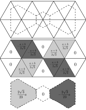
Figure 6: Defining $\mathcal{R}_{h}\boldsymbol{u}$ by averaging the normal components of $\boldsymbol{u}$ along the primary or dual cell edges can lead to inconsistently defined differential operators. Upper panel: the primary mesh consists of equilateral triangles, and the dual mesh consists of non-uniform but equiangular hexagons. The dual cell edge intersects the primary cell edge either at the mid-point or at the one-third point. Every two neighboring primary cell centers are equi-distant to the common edge that separates them. Middle panel: a non-diminishing scalar divergence field that results from averaging the normal components of $\boldsymbol{u}=(ay,\,bx)$ along dual cell edges. Lower panel: a non-diminishing scalar vorticity field that results from averaging the normal components of $\boldsymbol{u}=(ax,\,by)$ along the primary cell edges.

Remark 2.12.

It is tempting to define $\mathcal{R}_{h}\boldsymbol{u}$ as the average of the normal component of $\boldsymbol{u}$ along one of the edges ($\l_{e}$ or $d_{e}$, see Figure 3). However, it is also well-known in the finite volume literature ([34, 29] that volume or area or length averaging leads to inconsistently defined differential operators. In our terminologies, condition C1 of Definition 2.3 may be violated if the restriction operator $\mathcal{R}_{h}$ is defined this way. One-dimensional examples have been given in the two references just cited. Here we give a two-dimensional example, in which the primary mesh consists of equilateral triangles, and the dual mesh consists of non-uniform but equiangular hexagons (see the upper panel of Figure 6). Around each triangle, the dual cell edge (dashed line) intersects the primary cell edge (solid line) either at the one-third point, or at the mid-point. The triangular mesh is Voronoi in the sense that every two neighboring cell centers are equi-distant to the common edge between them, but the staggered meshes are not the classical Delaunay-Voronoi meshes, because the roles of the triangles and the roles of the hexagons are mutated. First, we discuss the case when the normal component of $\boldsymbol{u}$ is averaged along the dual cell edge (dashed lines). We let $\boldsymbol{u}=(ay,\,bx)$, where $a$ and $b$ are two arbitrary constants. The analytic divergence $\delta=u_{x}+v_{y}$ vanishes everywhere. The discrete divergence $\delta_{h}=\nabla_{h}\cdot\mathcal{R}_{h}\boldsymbol{u}$ is a piecewise constant function on the primary mesh, and it can take three values, $0$, $(a+b)/2\sqrt{3}$ and $-(a+b)/2\sqrt{3}$. The distribution pattern of these discrete values are shown in the middle panel of Figure 6. Clearly, for $a+b\neq 0$, $\delta_{h}$ does not converge to $\delta$ in the $L^{2}$-norm as the mesh refines. It only converges weakly. For the case of averaging along the primary cell edges (solid lines), we let $\boldsymbol{u}=(ax,\,by)$, again $a$, $b$ being arbitrary constants. The analytic vorticity $\omega=v_{x}-u_{y}$ vanishes everywhere. But the discrete vorticity $\omega_{h}=\nabla_{h}\times\mathcal{R}_{h}\boldsymbol{u}$, which are piecewise constant functions on the dual mesh, takes three possible values, $0$, $2\sqrt{3}a/23$ and $-2\sqrt{3}a/23$, and the distribution pattern of these discrete values is shown in the lower panel of Figure 6. It is clear that, for $a\neq 0$, the discrete vorticity $\omega_{h}$ does not converge to the analytic vorticity $\omega$ in the $L^{2}$-norm, as the mesh refines. It only converges weakly.

3 The linear incompressible Stokes problem

As in the previous section, we assume that $\Omega$ is an open, bounded, and simply-connected domain with piece-wise smooth boundaries. The incompressible Stokes problem reads

$$\left\{{\begin{aligned} -\Delta\boldsymbol{u}+\nabla p&=\boldsymbol{f},&&\Omega,\\ \nabla\cdot\boldsymbol{u}&=0,&&\Omega,\\ \boldsymbol{u}&=0,&&\partial\Omega.\end{aligned}}\right.$$ (3.1)

Using the vector identity

$$\Delta\boldsymbol{u}=\nabla(\nabla\cdot\boldsymbol{u})+\nabla^{\perp}(\nabla\times\boldsymbol{u}),$$ (3.2)

and the incompressibility condition, one derives the vorticity formulation of the Stokes problem,

$$\left\{{\begin{aligned} -\nabla^{\perp}\nabla\times\boldsymbol{u}+\nabla p&=\boldsymbol{f},&&\Omega,\\ \nabla\cdot\boldsymbol{u}&=0,&&\Omega,\\ \boldsymbol{u}&=0,&&\partial\Omega.\end{aligned}}\right.$$ (3.3)

Here, $\nabla^{\perp}=\mathbf{k}\times\nabla$, $\mathbf{k}$ being the upward unit vector, denotes the skewed gradient operator. We will use the vorticity formulation, since it highlights the role of vorticity, and seems most suitable for staggered-grid discretization techniques.

The natural functional space for the solution of the Stokes problem (3.1) is

$$V=\{\boldsymbol{u}\in H^{1}_{0}(\Omega)\,|\,\nabla\cdot\boldsymbol{u}=0\textrm{ in }\Omega\}.$$

It is a Hilbert space under the norm

$$\|\boldsymbol{u}\|_{V}^{2}=|\nabla\times\boldsymbol{u}|_{0}^{2}.$$ (3.4)

By integration by parts, we obtain the weak formulation of (3.1):

For each $\boldsymbol{f}\in L^{2}(\Omega)\times L^{2}(\Omega)$, find $\boldsymbol{u}\in V$ such that

$$(\nabla\times\boldsymbol{u},\,\nabla\times\boldsymbol{v})=(\boldsymbol{f},\,\boldsymbol{v})\quad\forall\boldsymbol{v}\in V.$$ (3.5)

It is clear that changes need to be made regarding the discrete function space $V_{h}$ in order to accommodate the incompressibility condition and the no-slip boundary condition, both present in the new function space $V$. The previous definition (2.25) of $V_{h}$ is changed to

$$V_{h}=\left\{u_{h}=\sum_{e=1}^{N_{e}}u_{e}\chi_{e}\mathbf{n}_{e}\,\biggr{|}\,\,\nabla_{h}\cdot u_{h}=0.\right\}$$ (3.6)

The discrete divergence operator $\nabla_{h}\cdot(\,)$ and the discrete curl operator $\widetilde{\nabla}_{h}\times(\,)$ are defined as before, but with $V_{h}$ defined as in (3.6), the edges on the boundary has no effect on either the divergence or the vorticity. The discrete Poincaré inequality still applies in this case, and $V_{h}$ is a Hilbert space with the norm

$$\|u_{h}\|_{V_{h}}\equiv|u_{h}|_{1,h}\equiv|\widetilde{\nabla}_{h}\times u_{h}|_{0}.$$ (3.7)

3.1 External approximation of $V$

Since all functions in $V$ are divergence free, there is a one-to-one correspondence between $V$ and $H^{2}_{0}(\Omega)$ ([32]). We let

$$F=L^{2}(\Omega)\times L^{2}(\Omega).$$

For each $\boldsymbol{u}\in V$, we let $\psi\in H^{2}_{0}(\Omega)$ and $\omega\in L^{2}(\Omega)$ such that

$$\boldsymbol{u}=\nabla^{\perp}\psi,\qquad\nabla\times\boldsymbol{u}=\omega.$$ (3.8)

Then we redefine the isomorphism $\Pi$ from $V$ into $F$ as

$$\Pi\boldsymbol{u}=(\psi,\,\omega)\in F,\qquad\forall\boldsymbol{u}\in V.$$ (3.9)

The space $F$ is endowed with the usual $L^{2}$-norm. In view of the norm for $V$, it is clear that $\Pi$ is an isomorphism from $V$ into $F$. It is important to note that the image of the operator $\Pi$ is not the whole space $F$. It is a nowhere dense, closed subspace of the latter. Given a vector function $(\psi,\,\omega)$ in $F$, there is no known method to determine whether it is the image of some element $\boldsymbol{u}$ in $V$, other than solving an elliptic or biharmonic equation. For this reason, we need a straightforward way of specifying a restriction operator that is convergent. The specifications for the meshes are the same as in Section 2.2. For this problem, we further assume that the primary cell edge and the dual cell edge bisect each other in the interior of the domain. This requirement is stronger than what is actually needed (see Remark 3.2).

Under the foregoing assumptions on the meshes, we now define the restriction operator $\mathcal{R}_{h}$. We only need to define $\mathcal{R}_{h}$ for a dense subset of functions of $V$, and the definition can then be extended to the whole space of $V$ according to a result in [33]. We let

$$\mathcal{V}=\{\boldsymbol{u}\in\mathcal{D}(\Omega)\,|\,\nabla\cdot\boldsymbol{u}=0\},$$ (3.10)

which is a dense subspace of $V$. For an arbitrary $\boldsymbol{u}\in\mathcal{V}$, there exists $\psi\in\mathcal{D}(\Omega)$ such that $\boldsymbol{u}=\nabla^{\perp}\psi$, and thus $\omega=\Delta\psi$. We then define the associated discrete scalar field as

$$\psi_{h}=\sum_{\nu=1}^{N_{v}}\psi_{\nu}\chi_{\nu},$$ (3.11)

with

$$\psi_{\nu} =\psi(x_{\nu}),$$ on interior dual cells, (3.12)

$$\psi_{\nu} =0,$$ on dual cells on the boundary, (3.13)

where $x_{\nu}$ is the coordinates for the center of dual cell $\nu$. We note that the function $\psi$ has compact support on $\Omega$, and therefore, if the grid resolution $h$ is fine enough, the specification (3.13) is consistent with (3.12). Finally, the restriction operator $\mathcal{R}_{h}$ on $\boldsymbol{u}\in\mathcal{V}$ is defined as

$$\mathcal{R}_{h}\boldsymbol{u}=\widetilde{\nabla}_{h}^{\perp}\psi_{h}.$$ (3.14)

That $\mathcal{R}_{h}\boldsymbol{u}$ is divergence free in the discrete sense is guaranteed by Lemma 2.6. It vanishes on the boundary thanks to the condition (3.13) and the definition (2.17) for the skewed gradient operator on the boundary.

To define the prolongation operator $\mathcal{P}_{h}$, we note that, by the virtue of Lemma 2.6, every $u_{h}\in V_{h}$ is represented by a scalar field $\psi\in\Psi_{h}$ via

$$u_{h}=\widetilde{\nabla}_{h}^{\perp}\psi_{h}.$$ (3.15)

The prolongation operator $\mathcal{P}_{h}$ is defined as

$$\mathcal{P}_{h}u_{h}=(\psi_{h},\,\widetilde{\nabla}_{h}\times u_{h}),\qquad\forall u_{h}\in V_{h}.$$ (3.16)

The external approximation of $V$ consists of the mapping pair $(F,\,\Pi)$ and the family of triplets $\{V_{h},\,\mathcal{R}_{h},\,\mathcal{P}_{h}\}_{h\in\mathcal{H}}$. Concerning this approximation we have the following claim.

Theorem 3.1.

The external approximation that consists of the function space $F$, the isomorphic mapping $\Pi$, and the family of triplets $\{V_{h},\,\mathcal{R}_{h},\,\mathcal{P}_{h}\}_{h\in\mathcal{H}}$ is a stable and convergent approximation of $V$.

Proof.

According to Definition 2.2, the approximation is stable if the prolongation operators $\mathcal{P}_{h}$ are stable, which is evidently the case, in view of the specifications (3.7) and (3.16), and the discrete Poincaré inequality.

The approximation is convergent if Conditions (C1) and (C2) of Definition 2.3 are met. According to [33], it is only necessary to verify Condition (C1) for the space $\mathcal{V}$. Let $\boldsymbol{u}\in\mathcal{V}$ and $\Pi\boldsymbol{u}=(\psi,\,\omega)\in F$, and let $\psi_{h}$ be defined as in (3.12)- (3.13). The (C1) condition is verified once we show that, as the grid resolution $h$ tends to zero, the discrete scalar field $\psi_{h}$ defined by (3.12)- (3.13) converges strongly to $\psi$ in $L^{2}(\Omega)$, and $\widetilde{\nabla}_{h}\times\widetilde{\nabla}_{h}^{\perp}\psi_{h}$ converges strongly to $\omega$ in $L^{2}(\Omega)$. The first claim can be easily verified by an application of the Taylor series expansion of $\psi$. The second claim reflects the consistency of the discrete Laplacian operator on this mesh. Indeed, we note that, because the primary cell edge $l_{e}$ and the dual cell edge $d_{e}$ bisect each other,

$$[\widetilde{\nabla}^{\perp}\psi_{h}]_{e}=\overline{\left(\frac{\partial\psi}{\partial t_{e}}\right)}^{d_{e}}+O(h^{2}),$$ (3.17)

where the overbar $\overline{\phantom{A}}^{d_{e}}$ denotes averaging along the dual cell $d_{e}$. Applying the discrete curl operator to the above, we obtain

$$[\widetilde{\nabla}_{h}\times\widetilde{\nabla}_{h}^{\perp}\psi_{h}]_{\nu}=\overline{(\Delta\psi)}^{A_{\nu}}+O(h),$$ (3.18)

with the overbar $\overline{\phantom{A}}^{A_{\nu}}$ denoting averaging over the dual cell $A_{\nu}$. The claim can then be authenticated by application of the Taylor series expansion to $\Delta\psi$.

For Condition (C2), we assume that a sequence $\{\mathcal{P}_{h}u_{h}\}_{h\in\mathcal{H}}$, with $u_{h}\in V_{h}$, converges weakly to an element $(\psi,\,\omega)\in F$, that is, as $h\longrightarrow 0$,

$$\mathcal{P}_{h}u_{h}\rightharpoonup(\psi,\,\omega)\qquad\textrm{weakly in }F,$$ (3.19)

which means that, according to definition (3.16),

$$\psi_{h} \rightharpoonup\psi\qquad\textrm{weakly in }L^{2}(\Omega),$$ (3.20)

$$\Delta_{h}\psi_{h} \rightharpoonup\omega\qquad\textrm{weakly in }L^{2}(\Omega).$$ (3.21)

Here, $\psi_{h}$ is a scalar field such that $u_{h}=\widetilde{\nabla}^{\perp}_{h}\psi_{h}$.

We claim that

$$\psi\in H^{2}(\Omega),$$ (3.22)

$$\Delta\psi=\omega, \Omega$$ (3.23)

$$\psi=\dfrac{\partial\psi}{\partial n}=0, \partial\Omega.$$ (3.24)

Once these properties are verified, we set $\boldsymbol{u}=\nabla^{\perp}\psi$. It is clear then that $\boldsymbol{u}\in V$ and $(\psi,\,\omega)=\Pi\boldsymbol{u}$.

We let

$$\psi_{h}^{\#} = \textrm{extension of }\psi_{h}\textrm{ outside }\Omega\textrm{ by zero},$$

$$\psi^{\#} = \textrm{extension of }\psi\textrm{ outside }\Omega\textrm{ by zero},$$

$$(\Delta_{h}\psi_{h})^{\#} = \textrm{extension of }\Delta_{h}\psi_{h}\textrm{ outside }\Omega\textrm{ by zero},$$

$$\omega^{\#} = \textrm{extension of }\omega\textrm{ outside }\Omega\textrm{ by zero}.$$

The mesh $\mathcal{T}_{h}$ is also extended outside $\Omega$, and the extended mesh $\mathcal{T}^{\#}_{h}$ satisfies the aforementioned requirements. We note that, thanks to the boundary conditions on $\psi_{h}$,

$$(\Delta_{h}\psi_{h})^{\#}=\Delta_{h}\psi_{h}^{\#}.$$ (3.25)

Convergences (3.20) and (3.21) imply that

$$\psi^{\#}_{h} \rightharpoonup\psi^{\#},\qquad\textrm{weakly in }L^{2}(\mathbb{R}^{2}).$$ (3.26)

$$\Delta_{h}\psi^{\#}_{h} \rightharpoonup\omega^{\#},\qquad\textrm{weakly in }L^{2}(\mathbb{R}^{2}).$$ (3.27)

We let $\psi^{\prime}\in\mathcal{D}(\mathbb{R}^{2})$, and let $\psi^{\prime}_{h}=\sum\psi^{\prime}(x_{\nu})\chi_{\nu}$. Thanks to the compact support of $\psi^{\prime}$, it can be shown in a similar fashion as in the verification of the (C1) condition above that

$$\psi^{\prime}_{h} \longrightarrow\psi^{\prime},\qquad\textrm{strongly in }L^{2}(\mathbb{R}^{2}).$$ (3.28)

$$\Delta_{h}\psi^{\prime}_{h} \longrightarrow\Delta\psi^{\prime},\qquad\textrm{strongly in }L^{2}(\mathbb{R}^{2}).$$ (3.29)

The following integration-by-parts formula holds for $\psi^{\#}_{h}$ and $\psi^{\prime}_{h}$,

$$(\psi^{\#}_{h},\,\Delta_{h}\psi^{\prime}_{h})=(\Delta_{h}\psi^{\#}_{h},\,\psi^{\prime}_{h}).$$ (3.30)

Thanks to the weak convergences (3.20) and (3.21) and the strong convergences (3.28) and (3.29), we can pass to the limit in (3.30) and obtain

$$(\psi^{\#},\,\Delta\psi^{\prime})=(\omega^{\#},\,\psi^{\prime}),$$ (3.31)

which implies that

$$\Delta\psi^{\#}=\omega^{\#}\qquad\textrm{in }\mathcal{D}^{\prime}(\mathbb{R}^{2}).$$ (3.32)

This relation, together with the fact that $\psi^{\#}\in L^{2}(\mathbb{R}^{2})$ and $\omega^{\#}\in L^{2}(\mathbb{R}^{2})$, implies that

$$\psi^{\#}\in H^{2}(\mathbb{R}^{2}).$$ (3.33)

Restricted to the domain $\Omega$, (3.33) and (3.32) imply (3.22) and (3.23), respectively. The boundary conditions (3.24) for $\psi$ follow from the fact that $\psi^{\#}\in H^{2}(\mathbb{R}^{2})$, and $\psi^{\#}$ vanishes entirely outside $\Omega$. ∎

Remark 3.2.

The bisecting requirement on the meshes can be relaxed without affecting the convergence conclusion of Theorem 3.1. Specifically, the C1 condition for convergence relies on the second order accuracy of $[\widetilde{\nabla}^{\perp}\psi_{h}]_{e}$ as an approximation to $\overline{(\partial\psi/\partial t_{e})}^{d_{e}}$. The same order of accuracy can still be achieved if we allow the intersection of the primary cell edge $l_{e}$ and the dual cell edge $d_{e}$ to depart from their mid-points by no more than $O(h^{2})$.

3.2 Convergence of the MAC scheme

The vorticity formulation (3.3) is most suitable for discretization on staggered grids, and this is the form that we will use. In discretizing the system, it is important to ensure that the external forcing $\boldsymbol{f}$ is also discretized in a consistent way. For the sake of the convergence proof later on, we discretize the forcing term using its scalar stream and potential functions. For each $\boldsymbol{f}\in L^{2}(\Omega)\times L^{2}(\Omega)$, we let $\psi^{f}\in H_{0}^{1}(\Omega)$ and $\phi^{f}\in H^{1}(\Omega)/\mathbb{R}$ be such that

$$\boldsymbol{f}=\nabla^{\perp}\psi^{f}+\nabla\phi^{f}.$$ (3.34)

By the famous Helmholtz decomposition theorem, the stream and potential functions always exist and are unique, for each vector field $\boldsymbol{f}$ in $L^{2}(\Omega)\times L^{2}(\Omega)$ (see [32]). The stream and potential functions are discretized on the dual and primary meshes, respectively, by averaging,

$$\psi^{f}_{h} =\sum_{\nu=1}^{N_{v}}\psi^{f}_{\nu}\chi_{\nu}, \textrm{with }\psi^{f}_{\nu} =\overline{\psi^{f}}^{A_{\nu}},$$ (3.35)

$$\phi^{f}_{h} =\sum_{i=1}^{N_{c}+N_{cb}}\phi^{f}_{i}\chi_{i}, \textrm{with }\phi^{f}_{i} =\overline{\phi^{f}}^{A_{i}}.$$ (3.36)

Employing the technique of approximation by smooth functions and the Taylor’s series expansion, we can show that the discrete scalar fields converge to the corresponding continuous fields in the $L^{2}$-norm, i.e.

$$\psi^{f}_{h} \longrightarrow\psi^{f} \textrm{strongly in }L^{2}(\Omega),$$ (3.37)

$$\phi^{f}_{h} \longrightarrow\phi^{f} \textrm{strongly in }L^{2}(\Omega).$$ (3.38)

With $\psi^{f}_{h}$ and $\phi^{f}_{h}$ defined as in (3.35) and (3.36), a discrete vector field can be specified,

$$f_{h}=\widetilde{\nabla}_{h}^{\perp}\psi^{f}_{h}+\nabla_{h}\phi^{f}_{h}.$$ (3.39)

We take $f_{h}$ as the discretization of the continuous vector forcing field $\boldsymbol{f}$.

The discrete problem can now be stated as follows.

For each $\boldsymbol{f}\in L^{2}(\Omega)\times L^{2}(\Omega)$, let $f_{h}$ be defined as in (3.39). Find $u_{h}\in V_{h}$ and $p_{h}\in\Phi_{h}$ such that

$$-[\widetilde{\nabla}_{h}^{\perp}\widetilde{\nabla}_{h}\times u_{h}]_{e}+[\nabla_{h}p_{h}]_{e}=f_{e},\qquad 1\leq e\leq N_{e}.$$ (3.40)

The incompressibility condition and the homogeneous boundary conditions on $u_{h}$ have been included in the specification of the space $V_{h}$. It is important to note that equation (3.40) holds on interior edges only. On boundary edges, the computation of $\widetilde{\nabla}^{\perp}_{h}\widetilde{\nabla}_{h}\times u_{h}$ will require boundary conditions for $\widetilde{\nabla}_{h}\times u_{h}$, which are not available a priori.

As for the continuous problem, we multiply (3.40) by $v_{h}\in V_{h}$ and integrate by parts, and noticing that $v_{h}=0$ along the boundary (see also Lemma 2.5, and the remarks following its proof), we obtain the variational form of the numerical scheme,

$$(\widetilde{\nabla}_{h}\times u_{h},\,\widetilde{\nabla}_{h}\times v_{h})=2(f_{h},\,v_{h}).$$ (3.41)

The term involving the pressure $p_{h}$ vanishes because of the incompressibility condition on $v_{h}$. The factor 2 on the right-hand side of (3.41) results from the integration-by-parts process. It can also be directly explained by the fact that the inner product on the right-hand side only involves the normal components of the vector fields. For $u_{h},\,v_{h}\in V_{h}$, we define the bilinear form

$$a_{h}(u_{h},\,v_{h})=(\widetilde{\nabla}_{h}\times u_{h},\,\widetilde{\nabla}_{h}\times v_{h}).$$ (3.42)

Then the variational form of the numerical scheme can be stated as follows.

For each $\boldsymbol{f}\in L^{2}(\Omega)\times L^{2}(\Omega)$, let $f_{h}$ be defined as in (3.39). Find $u_{h}\in V_{h}$ such that

$$a_{h}(u_{h},\,v_{h})=2(f_{h},\,v_{h}),\qquad\forall v_{h}\in V_{h}.$$ (3.43)

Given the norm (3.7) on $V_{h}$, the bilinear form $a_{h}(\cdot,\,\cdot)$ is coercive. Thus by Lax-Milgram theorem, for every discrete vector field $f_{h}$, there exists a unique $u_{h}\in V_{h}$ such that (3.43) holds. Noticing that $v_{h}=0$ on edges that intersects with the boundary, we integrate the left-hand side of (3.43) by parts to obtain

$$\left(-\widetilde{\nabla}_{h}^{\perp}\widetilde{\nabla}_{h}\times u_{h}-f_{h},\,v_{h}\right)=0,\qquad\forall v_{h}\in V_{h}.$$ (3.44)

We let $v_{h}=\widetilde{\nabla}_{h}^{\perp}\psi_{h}$ for some $\psi_{h}\in\Psi_{h}$ that vanishes on dual cells that border the boundary. We replace $v_{h}$ by $\widetilde{\nabla}_{h}^{\perp}\psi_{h}$ in (3.44), and integrate by parts again to obtain

$$\left(\widetilde{\nabla}_{h}\times(-\widetilde{\nabla}_{h}^{\perp}\widetilde{\nabla}_{h}\times u_{h}-f_{h}),\,\psi_{h}\right)=0.$$ (3.45)

Thanks to the arbitrariness of $\psi_{h}$, equation (3.45) implies that

$$\left[\widetilde{\nabla}_{h}\times(-\widetilde{\nabla}_{h}^{\perp}\widetilde{\nabla}_{h}\times u_{h}-f_{h})\right]_{\nu}=0,\qquad\textrm{on interior dual cells.}$$ (3.46)

Following the same line of arguments as in the proof of Lemma 2.7, we can show that there exists $p_{h}\in\Phi_{h}$, unique up to a constant, such that

$$\left[-\widetilde{\nabla}_{h}^{\perp}\widetilde{\nabla}_{h}\times u_{h}+\nabla_{h}p_{h}\right]_{e}=f_{e},\qquad\textrm{on interior edges.}$$ (3.47)

Thus the pressure is recovered, and (3.40) holds true.

Remark 3.3.

The existence and uniqueness of a discrete solution to the system (3.40) can also be established from the point of view of a square linear system. Indeed, in practice, the equations in (3.40) are coupled with the incompressibility constraints on $u_{h}$,

$$[\nabla_{h}\cdot u_{h}]_{i}=0,\qquad 1\leq i\leq N_{c}+N_{cb}.$$ (3.48)

One of these equations is redundant, and should be dropped. Thus we have $N_{e}+N_{c}+N_{cb}-1$ equations, for $N_{e}+N_{c}+N_{cb}$ unknowns ($u_{e}$’s with $1\leq e\leq N_{e}$ and $p_{i}$’s with $1\leq i\leq N_{c}+N_{cb}$). There is one more unknown than the number of equations, which is a reflection of the fact that if $p_{h}$ is a solution of (3.40), then so is $p_{h}+c$ for any constant $c$. To uniquely determine the pressure, we may impose an extra constraint on $p_{h}$, such as

$$\int_{\Omega}p_{h}dx=0.$$ (3.49)

The final system has $N_{e}+N_{c}+N_{cb}$ unknowns, and $N_{e}+N_{c}+N_{cb}$ equations, and is a square linear system. For a finite dimensional square linear system, uniqueness is equivalent to solvability. Thus we can claim unique solvability for the system (3.40), (3.48) and (3.49) once we show that the only solutions corresponding to $f_{h}=0$ is the trivial solution $u_{h}=0$ and $p_{h}=0$. If $f_{h}=0$, then the only solution to (3.43) is $u_{h}=0$, thanks to the coercivity of the bilinear form $a_{h}(\cdot,\,\cdot)$. With $u_{h}=0$ and $f_{h}=0$ in (3.40), we derive that $\nabla_{h}p_{h}=0$, which means that $p_{h}$ is a constant over the entire domain. The constraint (3.49) implies that this constant must be zero. Hence, for every $f_{h}$, the numerical scheme (3.40) has a unique solution.

We now obtain a energy bound on the discrete solution in terms the data. To this end, we set $v_{h}=u_{h}$ in (3.43),

$$|u_{h}|^{2}_{1,h}\equiv|\widetilde{\nabla}_{h}\times u_{h}|_{0,h}^{2}=2(f_{h},\,u_{h}).$$ (3.50)

To estimate the right-hand side, we substitute (3.39) for $f_{h}$, and integrate by parts using formulae (2.37) and (2.38) to obtain

$$|u_{h}|_{1,h}^{2}=-(\widetilde{\nabla}_{h}\times u_{h},\,\psi^{f}_{h}).$$ (3.51)

The term involving $\phi^{f}_{h}$ has vanished due to the incompressibility condition on $u_{h}$. An simple application of the Cauchy-Schwarz inequality yields

$$|u_{h}|_{1,h}\leq C|\psi^{f}_{h}|_{0}.$$ (3.52)

Combining this equation with the fact that $\psi^{f}_{h}$ converges to $\psi^{f}$ as $h$ converges to zero, we derive that

$$|u_{h}|_{1,h}\leq C|\psi^{f}|_{0}+K,$$ (3.53)

where $C$ and $K$ are constants that are independent of $h$.

The results are summarized in the following theorem.

Theorem 3.4.

For each $\boldsymbol{f}\in L^{2}(\Omega)\times L^{2}(\Omega)$, let $f_{h}$ be defined as in (3.39). There exists a unique $u_{h}\in V_{h}$, and a $p_{h}\in\Phi_{h}$, unique up to a constant, such that (3.40) holds. In addition, the discrete solution $u_{h}$ is bounded,

$$|u_{h}|_{1,h}\leq C|\psi^{f}|_{0}+K,$$ (3.54)

where $C$ and $K$ are constants independent of the grid resolution $h$.

We next show that the discrete solution $u_{h}$ of (3.43) converges, and the limit is a solution of the continuous problem (3.5).

Theorem 3.5.

For each $\boldsymbol{f}\in L^{2}(\Omega)\times L^{2}(\Omega)$, let $f_{h}$ be defined as in (3.39), and let $u_{h}$ be the unique solution of (3.43). Then there exists a unique $\boldsymbol{u}\in V$ such that, as the grid resolution refines,

$$\mathcal{P}_{h}u_{h}\longrightarrow\Pi\boldsymbol{u}\qquad\textrm{strongly in }F,$$ (3.55)

and $\boldsymbol{u}$ solves the variational problem (3.5).

Proof.

We first show that the discrete solutions $u_{h}$ converge. By the boundedness (3.54) of $u_{h}$, there exists $(\psi,\,\omega)\in F$ and a subsequence $u_{h^{\prime}}$ such that, as the grid resolution refines,

$$\mathcal{P}_{h^{\prime}}u_{h^{\prime}}\equiv(\psi_{h^{\prime}},\,\widetilde{\nabla}_{h^{\prime}}\times u_{h^{\prime}})\rightharpoonup(\psi,\,\omega)\quad\textrm{weakly in }F.$$ (3.56)

By the (C2) condition for a convergent approximation, there exists $\boldsymbol{u}\in V$ such that

$$(\psi,\,\omega)=\Pi\boldsymbol{u}.$$

We next show that $\boldsymbol{u}$ solves the continuous variational problem (3.5). We let $\boldsymbol{v}\in\mathcal{V}\subset V$, $v_{h^{\prime}}=\mathcal{R}_{h^{\prime}}\boldsymbol{v}$. By the (C1) condition for a convergent approximation,

$$\mathcal{P}_{h^{\prime}}\mathcal{R}_{h^{\prime}}\boldsymbol{v}\equiv(\widetilde{\psi}_{h^{\prime}},\,\widetilde{\nabla}_{h^{\prime}}\times v_{h^{\prime}})\longrightarrow(\widetilde{\psi},\,\nabla\times\boldsymbol{v})\quad\textrm{strongly in }F.$$ (3.57)

The discrete variational problem (3.43) holds with these $v_{h^{\prime}}$ as the test functions,

$$(\widetilde{\nabla}_{h^{\prime}}\times u_{h^{\prime}},\,\widetilde{\nabla}_{h^{\prime}}\times v_{h^{\prime}})=2(f_{h^{\prime}},\,v_{h^{\prime}}).$$ (3.58)

Replacing the $f_{h^{\prime}}$ on the right-hand side by $\widetilde{\nabla}_{h^{\prime}}^{\perp}\psi^{f}_{h^{\prime}}+\nabla_{h^{\prime}}\phi^{f}_{h^{\prime}}$, and integrating by parts, we obtain

$$(\widetilde{\nabla}_{h^{\prime}}\times u_{h^{\prime}},\,\widetilde{\nabla}_{h^{\prime}}\times v_{h^{\prime}})=-(\psi^{f}_{h^{\prime}},\,\widetilde{\nabla}_{h^{\prime}}\times v_{h^{\prime}}).$$ (3.59)

In view of the convergences (3.37), (3.56), and (3.57), we pass to the limit in (3.59) by letting $h^{\prime}\longrightarrow 0$, and obtain

$$(\nabla\times\boldsymbol{u},\,\nabla\times\boldsymbol{v})=-(\psi^{f},\,\nabla\times\boldsymbol{v}).$$ (3.60)

Integrating by parts again on the right-hand side yields

$$(\nabla\times\boldsymbol{u},\,\nabla\times\boldsymbol{v})=(\boldsymbol{f},\,\boldsymbol{v}).$$ (3.61)

Since $\mathcal{V}$ is dense in $V$, the above holds for every $\boldsymbol{v}\in V$, which confirms that $\boldsymbol{u}$ is a solution of (3.5).

Finally, we show that the convergence (3.56) holds for the whole sequence $u_{h}$, and in the strong topology of $F$. The solution $\boldsymbol{u}$ of (3.5) is necessarily unique. Then by a contradiction argument, the convergence (3.56) must hold for the entire sequence of $u_{h}$. We now examine the difference $u_{h}-\mathcal{R}_{h}\boldsymbol{u}$ in the semi-$H^{1}$ norm of $V_{h}$.

$$|u_{h}-\mathcal{R}_{h}\boldsymbol{u}|_{1,h}^{2} =a_{h}(u_{h}-\mathcal{R}_{h}\boldsymbol{u},\,u_{h}-\mathcal{R}_{h}\boldsymbol{u})$$

$$=a_{h}(u_{h},\,u_{h})+a_{h}(\mathcal{R}_{h}\boldsymbol{u},\,\mathcal{R}_{h}\boldsymbol{u})-2a_{h}(u_{h},\,\mathcal{R}_{h}\boldsymbol{u})$$

$$=2(f_{h},\,u_{h})+(\widetilde{\nabla}_{h}\times\mathcal{R}_{h}\boldsymbol{u},\,\widetilde{\nabla}_{h}\times\mathcal{R}_{h}\boldsymbol{u})-4(f_{h},\,\mathcal{R}_{h}\boldsymbol{u})$$

We let $\widehat{\psi}_{h}\in\Psi_{h}$ be such that

$$\mathcal{R}_{h}\boldsymbol{u} =\widetilde{\nabla}_{h}^{\perp}\widehat{\psi}_{h}.$$

Then, according to Theorem 3.1,

$$\mathcal{P}_{h}\mathcal{R}_{h}\boldsymbol{u}\equiv(\widehat{\psi}_{h},\,\widetilde{\nabla}_{h}\times\mathcal{R}_{h}\boldsymbol{u})\longrightarrow(\psi,\,\omega)=\Pi\boldsymbol{u}\quad\textrm{strongly in }F.$$ (3.62)

This relation, together with (3.37) and (3.56), imply that

$$2(f_{h},\,u_{h})=-(\psi^{f}_{h},\,\nabla_{h}\times u_{h}) \longrightarrow-(\psi^{f}_{h},\,\nabla\times\boldsymbol{u})=(\nabla^{\perp}\psi^{f},\,\boldsymbol{u})=(\boldsymbol{f},\,\boldsymbol{u}),$$

$$4(f_{h},\,\mathcal{R}_{h}\boldsymbol{u})=-2(\psi^{f}_{h},\,\widetilde{\nabla}_{h}\times\mathcal{R}_{h}\boldsymbol{u}) \longrightarrow-2(\psi^{f},\,\nabla\times\boldsymbol{u})=2(\nabla^{\perp}\psi^{f},\,\boldsymbol{u})=2(\boldsymbol{f},\,\boldsymbol{u}).$$

The strong convergence of $\widetilde{\nabla}_{h}\times\mathcal{R}_{h}\boldsymbol{u}$ to $\nabla\times\boldsymbol{u}$ in $L^{2}(\Omega)$ also implies that

$$(\widetilde{\nabla}_{h}\times\mathcal{R}_{h}\boldsymbol{u},\,\widetilde{\nabla}_{h}\times\mathcal{R}_{h}\boldsymbol{u}) \longrightarrow(\nabla\times\boldsymbol{u},\,\nabla\times\boldsymbol{u}).$$

Hence we have

$$|u_{h}-\mathcal{R}_{h}\boldsymbol{u}|_{1,h}^{2}\longrightarrow(\nabla\times\boldsymbol{u},\,\nabla\times\boldsymbol{u})-(\boldsymbol{f},\,\boldsymbol{u})=0.$$ (3.63)

The convergence (3.55) follows from (3.63) and the following observation,

$$|\mathcal{P}_{h}u_{h}-\Pi\boldsymbol{u}|_{0} \leq|\mathcal{P}_{h}u_{h}-\mathcal{P}_{h}\mathcal{R}_{h}\boldsymbol{u}|_{0}+|\mathcal{P}_{h}\mathcal{R}_{h}\boldsymbol{u}-\Pi\boldsymbol{u}|_{0}$$

$$\leq|\mathcal{P}_{h}|\cdot|u_{h}-\mathcal{R}_{h}\boldsymbol{u}|_{1,h}+|\mathcal{P}_{h}\mathcal{R}_{h}\boldsymbol{u}-\Pi\boldsymbol{u}|_{0}.$$

∎

4 Concluding remarks

In this article, we present a new framework for analyzing staggered-grid schemes on unstructured meshes. The framework employs the concept of external approximation to address the challenge that comes with the use of piecewise constant functions in FD/FV schemes. The framework uses vorticity and/or divergence to gauge the convergence of the numerical schemes. Vorticity and divergence are two fundamental quantities of fluid dynamics, and the performance of numerical schemes in approximating these quantities is of great interest, both theoretically and practically. In this work, we demonstrate the construction and analysis of an external approximation of the vector-valued function space $H^{\mathrm{div}}_{0}(\Omega)\cap H^{\mathrm{curl}}(\Omega)$. The external approximation is shown to be stable and convergent under the general orthogonal and convex assumptions on the primary and dual meshes. We also apply the framework to prove that the discrete solutions of the MAC scheme for the classical incompressible Stokes problem on unstructured meshes converge to the true solution, under an extra assumption that the primary cell edge and the dual cell edge nearly bisect each other. More precisely, the conclusion remains valid if the point of intersection between the primary cell edge and the dual cell edge departs from their mid-points by at most $O(h^{2})$.

It is not known whether the just mentioned convergence result for the Stokes problem still holds without the bisection assumption at all. It would be a highly desirable outcome if the assumption can be further weakened so that only the primary cell edge bisects the dual cell edge (or the other way around). In that case, the theoretical result will cover a wider range of meshes, including the famous Delaunay-Voronoi tessellations ([35]).

The current work is motivated by our study of the staggered-grid schemes for the shallow water equations ([17], [36]). So far, studies on this topic, including ours, have largely been computational and experimental ([2], [37], [16], [38]). Theoretical study, to establish the existence, uniqueness, and convergence of the discrete solutions, is vital to ensure that the schemes perform under the most general conditions. We believe that the framework presented in this work is suitable for this task. So far, this framework has only been applied to the incompressible Stokes problem. In order to apply the framework to nonlinear problems, we envision that new results and new techniques must be developed, such as the compactness of the discrete function spaces. To facilitate such development, and to make progress towards our ultimate goal, we will study a hierarchy of fluid models, with increasing complexity and relevance to geophysical flows, such as the stationary Navier-Stokes equations, the compressible Stokes problem, etc. Work on these models will be reported in future publications.

References

References

- [1] F. H. Harlow, J. E. Welch, Numerical Calculation of Time-Dependent Viscous Incompressible Flow of Fluid with Free Surface, Physics of Fluids 8 (12) (1965) 2182–2189.
- [2] A. Arakawa, V. R. Lamb, Computational design of the basic dynamical processes of the UCLA General Circulation Model, Methods Cornput, Methods in computational physics 17 (1977) 173–265.
- [3] P. Wesseling, Principles of computational fluid dynamics, Vol. 29 of Springer Series in Computational Mathematics, Springer-Verlag, Berlin, Berlin, Heidelberg, 2001.
- [4] F. H. Harlow, A. A. Amsden, Numerical calculation of almost incompressible flow, Journal of Computational Physics 3 (1) (1968) 80–93.
- [5] F. H. Harlow, A. A. Amsden, A numerical fluid dynamics calculation method for all flow speeds, Journal of Computational Physics 8 (2) (1971) 197–213.
- [6] H. Bijl, P. Wesseling, A unified method for computing incompressible and compressible flows in boundary-fitted coordinates, Journal of Computational Physics 141 (2) (1998) 153–173.
- [7] R. I. Issa, A. D. Gosman, A. P. Watkins, The computation of compressible and incompressible recirculating flows by a noniterative implicit scheme, Journal of Computational Physics 62 (1) (1986) 66–82.
- [8] K. C. Karki, S. V. Patankar, Pressure based calculation procedure for viscous flows at all speedsin arbitrary configurations, AIAA Journal 27 (9) (1989) 1167–1174.
- [9] D. R. van der Heul, C. Vuik, P. Wesseling, A conservative pressure-correction method for flow at all speeds, Comput. & Fluids 32 (8) (2003) 1113–1132.
- [10] I. Wenneker, A. Segal, P. Wesseling, A Mach-uniform unstructured staggered grid method, International Journal for Numerical Methods in Fluids 40 (9) (2002) 1209–1235.
- [11] W. C. Skamarock, A Linear Analysis of the NCAR CCSM Finite-Volume Dynamical Core, Month. Weath. Rev. 136 (6) (2008) 2112–2119.
- [12] J. Thuburn, Numerical wave propagation on the hexagonal C-grid, Journal of Computational Physics 227 (11) (2008) 5836–5858.
- [13] A. Gassmann, Inspection of hexagonal and triangular C-grid discretizations of the shallow water equations, Journal of Computational Physics 230 (7) (2011) 2706–2721.
- [14] A. Gassmann, A global hexagonal C-grid non-hydrostatic dynamical core (ICON-IAP) designed for energetic consistency, Quarterly Journal of the Royal Meteorological Society 139 (670) (2012) 152–175.
- [15] J. Thuburn, T. Ringler, W. Skamarock, J. Klemp, Numerical representation of geostrophic modes on arbitrarily structured C-grids, Journal of Computational Physics 228 (22) (2009) 8321–8335.
- [16] T. D. Ringler, J. Thuburn, J. B. Klemp, W. C. Skamarock, A unified approach to energy conservation and potential vorticity dynamics for arbitrarily-structured C-grids, Journal of Computational Physics 229 (9) (2010) 3065–3090.
- [17] Q. Chen, T. Ringler, M. Gunzburger, A co-volume scheme for the rotating shallow water equations on conforming non-orthogonal grids, Journal of Computational Physics 240 (2013) 174–197.
- [18] V. Girault, A combined finite element and marker and cell method for solving Navier-Stokes equations, Numer. Math. 26 (1) (1976) 39–59.
- [19] R. A. Nicolaides, X. Wu, Analysis and convergence of the MAC scheme. II. Navier-Stokes equations, Math. Comp. 65 (213) (1996) 29–44.
- [20] G. Kanschat, Divergence-free discontinuous Galerkin schemes for the Stokes equations and the MAC scheme, International Journal for Numerical Methods in Fluids 56 (7) (2008) 941–950.
- [21] R. Eymard, T. Gallouët, R. Herbin, J.-C. Latché, Convergence of the MAC scheme for the compressible Stokes equations, SIAM Journal on Numerical Analysis 48 (6) (2010) 2218–2246.
- [22] E. Chénier, R. Eymard, T. Gallouët, R. Herbin, An extension of the MAC scheme to locally refined meshes: convergence analysis for the full tensor time-dependent Navier–Stokes equations, Calcolo 52 (1) (2012) 1–39.
- [23] W. E, J.-G. Liu, Projection method. III. Spatial discretization on the staggered grid, Math. Comp. 71 (237) (2002) 27–47 (electronic).
- [24] R. A. Nicolaides, Analysis and Convergence of the MAC Scheme I. The Linear Problem, SIAM Journal on Numerical Analysis 29 (6) (1992) pp. 1579–1591.
- [25] S. H. Chou, Analysis and convergence of a covolume method for the generalized Stokes problem, Math. Comp. 66 (217) (1997) 85–104.
- [26] J. Céa, Approximation variationnelle des problèmes aux limites, Ann. Inst. Fourier (Grenoble) 14 (fasc. 2) (1964) 345–444.
- [27] J.-P. Aubin, Approximation of elliptic boundary-value problems, Wiley-Interscience [A division of John Wiley & Sons, Inc.], New York-London-Sydney, 1972.
- [28] R. Temam, Navier-Stokes equations, AMS Chelsea Publishing, Providence, RI, 2001.
- [29] S. Faure, D. Pham, R. Temam, Comparison of finite volume and finite difference methods and application, Anal. Appl. (Singap.) 4 (2) (2006) 163–208.
- [30] G.-M. Gie, R. Temam, Convergence of a cell-centered finite volume method and application to elliptic equations, Int. J. Numer. Anal. Model. 12 (3) (2015) 536–566.
- [31] R. Eymard, J. Fuhrmann, A. Linke, On MAC schemes on triangular delaunay meshes, their convergence and application to coupled flow problems, Numer. Methods Partial Differential Eq. 30 (4) (2014) 1397–1424.
- [32] V. Girault, P. Raviart, Finite element methods for Navier-Stokes equations: theory and algorithms, Springer-Verlag, Berlin, New York, 1986.
- [33] R. Temam, Numerical Analysis, Kluwer-Springer-Verlag, 1980.
- [34] R. Eymard, T. Gallouët, R. Herbin, Finite volume methods, in: Handbook of numerical analysis, Vol. VII, North-Holland, Amsterdam, 2000, pp. 713–1020.
- [35] Q. Du, V. Faber, M. Gunzburger, Centroidal Voronoi tessellations: applications and algorithms, SIAM Review 41 (4) (1999) 637–676 (electronic).
- [36] Q. Chen, On staggering techniques and the non-staggered Z-grid scheme, Numer. Math. 132 (1) (2016) 1–21.
- [37] D. Randall, Geostrophic adjustment and the finite-difference shallow-water equations, Month. Weath. Rev. 122 (6) (1994) 1371–1377.
- [38] D. Y. Le Roux, Spurious inertial oscillations in shallow-water models, Journal of Computational Physics 231 (24) (2012) 7959–7987.