Ring dark and anti-dark solitons in nonlocal media

Abstract

Ring dark and anti-dark solitons in nonlocal media are found. These structures have, respectively, the form of annular dips or humps on top of a stable continuous-wave background, and exist in a weak or strong nonlocality regime, defined by the sign of a characteristic parameter. It is demonstrated analytically that these solitons satisfy an effective cylindrical Kadomtsev-Petviashvilli (aka Johnson’s) equation and, as such, can be written explicitly in closed form. Numerical simulations show that they propagate undistorted and undergo quasi-elastic collisions, attesting to their stability properties.

In nonlinear optics, spatial dark solitons are known to be intensity dips, with a phase-jump across the intensity minimum, on top of a continuous-wave (cw) background beam. These structures may exist in bulk media and waveguides, due to the balance between diffraction and defocusing nonlinearity, and have been proposed for potential applications in photonics as adjustable waveguides for weak signals Kivshar and Luther-Davies (1998).

In the two-dimensional (2D) geometry, spatial dark solitons, in the form of stripes, are prone to the transverse modulation instability (MI) Kuznetsov and Turitsyn (1998), which leads to their bending and their eventual decay into vortices Tikhonenko et al. (1996). However, the instability band of the dark soliton stripes, may be suppressed if the stripe is bent so as to form a ring of particular length. This idea led to the introduction of ring dark solitons (RDSs) Kivshar and Yang (1994), whose properties have been studied both in theory Frantzeskakis and Malomed (1999); Nistazakis et al. (2001a) and in experiments Dreischuh et al. (2002), and potential applications of RDS to parallel guiding of signal beams were proposed Dreischuh et al. (1996). RDSs have also been predicted to occur in other physically relevant contexts, such as atomic Bose-Einstein condensates Theocharis et al. (2003) and polariton superfluids Rodrigues et al. (2014); Dominici et al. (2013).

While the above results rely on the study of nonlinear Schrödinger (NLS) models with a local nonlinearity, there exist many physical settings where the use of NLS models with a nonlocal nonlinearity are more appropriate. This occurs, e.g., in media featuring strong thermal nonlinearity Krolikowski et al. (2004) or in nematic liquid crystals Alberucci et al. (2014), where the nonlinear contribution to the refractive index depends on the intensity distribution in the transverse plane. It has been shown that dark solitons in one-dimensional (1D) settings exist in media with a defocusing nonlocal nonlinearity Kartashov and Torner (2007); Kong et al. (2010); Piccardi et al. (2011); Assanto et al. (2011); Pu et al. (2012); Horikis (2015) while, in the case of stripes, transverse MI may be suppressed due to the nonlocality Armaroli et al. (2009). The smoothing effect of the nonlocal response was shown to occur even in the case of shock wave formation Armaroli et al. (2009); Ghofraniha et al. (2007); Assanto et al. (2008); Xu et al. (2015), or give rise to stable 2D solitons Assanto (2012). Here we should note that, generally, pertinent nonlocal models do not possess soliton solutions in explicit form (other than the weakly nonlinear limit Królikowski and Bang (2000)). As such, various techniques have been used to analyze soliton dynamics and interactions, with the most common one being the variational approximation, where a particular form of the solution is chosen Peccianti and Assanto (2012); Alberucci and Assanto (2013); Assanto et al. (2009); Sciberras et al. (2014); Alberucci et al. (2014). However, to the best of our knowledge, RDSs in nonlocal media have not been considered so far.

It is the purpose of this article to study RDSs and ring anti-dark solitons (RASs) in nonlocal media. These structures have, respectively, the form of annular dips or humps on top of a stable cw background, and exist in a weak or strong nonlocality regime, defined by the sign of a characteristic parameter. Using a multiscale asymptotic expansion technique, we find that RDSs and RASs obey an effective Johnson’s equation, that models ring-shaped waves in shallow water Johnson (1980). We also perform direct simulations to show that RDSs and RASs propagate undistorted and undergo quasi-elastic collisions.

Light propagation in nonlocal media is governed by the following dimensionless model Kartashov and Torner (2007); Alberucci et al. (2014); Peccianti and Assanto (2012); Assanto (2012); Ghofraniha et al. (2007):

$$i\frac{{\partial u}}{{\partial z}}+\frac{1}{2}{\nabla^{2}}u-2\eta u=0,$$ (1a)

$$\nu{\nabla^{2}}\eta-2\eta=-2|u{|^{2}},$$ (1b)

with the transverse Laplacian in cylindrical geometry being: $\displaystyle{\nabla^{2}}=\frac{{{\partial^{2}}}}{{{\partial}r^{2}}}+\frac{1}{r}\frac{\partial}{{\partial r}}+\frac{1}{{{r^{2}}}}\frac{{{\partial^{2}}}}{{\partial{\theta^{2}}}}$. Here, $u=u(z,r,\theta)$ is the complex electric field envelope, $\eta=\eta(z,r,\theta)$ is the optical refractive index, and the parameter $\nu$ stands for the strength of nonlocality. Notice that two interesting limits are possible: the local limit, with $\nu$ small, where (1) reduce to a NLS-type equation with saturable nonlinearity Reinbert et al. (2006), and the nonlocal limit, with $\nu$ large. Here, we will treat $\nu$ as an arbitrary parameter.

We start by expressing functions $u$ and $\eta$ as Horikis (2015); Horikis and Frantzeskakis (2014):

$$u={u_{b}}(z)v(r,\theta,z)={u_{0}}{e^{-2iu_{0}^{2}{\kern 1.0pt}z}}v(r,\theta,z),$$

$$\eta={\eta_{b}}(z)w(r,\theta,z)=u_{0}^{2}w(r,\theta,z),$$

where $u_{0}$ is an arbitrary real constant, while $u_{b}(z)=u_{0}\exp(-2iu_{0}^{2}{\kern 1.0pt}z)$ and $\eta_{b}(z)=u_{0}^{2}$ form the cw background solution of (1) so that $v$ and $w$ satisfy:

$$i\frac{{\partial v}}{{\partial z}}+\frac{1}{2}{\nabla^{2}}v-2\eta_{b}(w-1)v=0,$$ (2a)

$$\nu{\nabla^{2}}w-2w=-2|v|^{2}.$$ (2b)

By doing so, we have now fixed constant unit boundary conditions at infinity and the asymptotic analysis for the determination of $v$ and $w$ may be directly applied. However, before proceeding further, it is relevant to investigate if the cw background is subject to MI. We thus perform a standard MI analysis, assuming small perturbations of $u_{b}(z)$ and $\eta_{b}(z)$ behaving like $\exp[i(k_{z}z+\boldsymbol{k}_{\perp}\cdot\boldsymbol{r}_{\perp})]$. Then, it is found that the longitudinal and transverse perturbation wavenumbers $k_{z}$ and $\boldsymbol{k}_{\perp}$ obey the dispersion relation: $k_{z}^{2}=2u_{0}^{2}\boldsymbol{k}_{\perp}^{2}\left[1+(1/2)\boldsymbol{k}_{\perp}^{2}\right]^{-1}+(1/4)\boldsymbol{k}_{\perp}^{4}.$ This equation shows that $k_{z}$ is always real and, thus, the cw solution is modulationally stable for the considered model (note that, generally, for certain response functions, nonlocality could possibly lead to MI even in the defocusing case Krolikowski et al. (2001)).

Next, we use the Madelung transformation $v=\rho e^{i\phi}$ (where real functions $\rho$ and $\phi$ denote the amplitude and phase of $v$), and obtain from (2) the following system:

$$\rho\frac{{\partial\phi}}{{\partial z}}-\frac{1}{2}{\nabla^{2}}\rho+\frac{1}{2}\rho{\left({\frac{{\partial\phi}}{{\partial r}}}\right)^{2}}+\frac{1}{{2{r^{2}}}}{\left({\frac{{\partial\phi}}{{\partial\theta}}}\right)^{2}}+2{\eta_{b}}(w-1)\rho=0,$$ (3a)

$$\frac{{\partial\rho}}{{\partial z}}+\frac{1}{2}\rho{\nabla^{2}}\phi+\frac{{\partial\rho}}{{\partial r}}\frac{{\partial\phi}}{{\partial r}}+\frac{1}{{{r^{2}}}}\frac{{\partial\rho}}{{\partial\theta}}\frac{{\partial\phi}}{{\partial\theta}}=0,$$ (3b)

$$\nu{\nabla^{2}}w-2w=-2{\rho^{2}}.$$ (3c)

Seek, now, small-amplitude solutions on top of the cw background in the form of the asymptotic expansions:

$$\rho=\sum_{j=0}^{\infty}{\varepsilon^{2j}}\rho_{2j},\quad\phi=\sum_{j=0}^{\infty}{\varepsilon^{2j+1}}\phi_{2j+1},\quad w=\sum_{j=0}^{\infty}{\varepsilon^{2j}}w_{2j},$$

where the unknown functions depend on the slow variables $R=\varepsilon(r-Cz)$ (where $C$ is the wave velocity), $\Theta=\theta/\varepsilon$, and $Z=\varepsilon^{3}z$. Substituting these expansions to (3) we obtain a hierarchy of coupled systems. To leading order in $\varepsilon$, i.e., for $O(\varepsilon^{-4})$ and $O(\varepsilon^{-3})$, a system of linear equations is obtained:

$$\left.{\begin{array}[]{c}\displaystyle{2u_{0}^{2}{w_{2}}-C\frac{{\partial{\phi_{1}}}}{{\partial R}}=0,}\\[6.0pt] \displaystyle{-2C\frac{{\partial{\rho_{2}}}}{{\partial R}}+\frac{{{\partial^{2}}{\phi_{1}}}}{{\partial{R^{2}}}}=0,}\\[3.0pt] \displaystyle{{w_{2}}=2{\rho_{2}},}\end{array}}\right\}\Leftrightarrow\left\{{\begin{array}[]{c}\displaystyle{\frac{{\partial{\phi_{1}}}}{{\partial R}}=\frac{{4u_{0}^{2}}}{{C}}{\rho_{2}}},\\[6.0pt] \displaystyle{C^{2}}=2u_{0}^{2},\\[3.0pt] \displaystyle{{w_{2}}=2{\rho_{2}}}.\end{array}}\right.$$ (10)

Notice that the velocity $C$, determined by (10), may have two signs, corresponding to outward or inward propagating ring solitons (see below). Next, at $O(\varepsilon^{1})$ and $O(\varepsilon^{-2})$ we get:

$$2{C^{2}}{w_{4}}+4{C^{2}}\rho_{2}^{2}+2\frac{{\partial{\phi_{1}}}}{{\partial Z}}-2C\frac{{\partial{\phi_{3}}}}{{\partial R}}-\frac{{{\partial^{2}}{\rho_{2}}}}{{\partial{R^{2}}}}=0,$$ (11)

$${w_{4}}=\rho_{2}^{2}+2{\rho_{4}}+\nu\frac{{{\partial^{2}}{\rho_{2}}}}{{\partial{R^{2}}}},$$ (12)

and at $O(\varepsilon^{-1})$:

$$2{C^{2}}{Z^{2}}\frac{{\partial{\rho_{2}}}}{{\partial Z}}+\frac{{{\partial^{2}}{\phi_{1}}}}{{\partial{\Theta^{2}}}}-4{C^{2}}RZ\frac{{\partial{\rho_{2}}}}{{\partial R}}-2{C^{3}}{Z^{2}}\frac{{\partial{\rho_{4}}}}{{\partial R}}+2CRZ\frac{{{\partial^{2}}{\phi_{1}}}}{{\partial{R^{2}}}}$$

$$+{C^{2}}Z{\rho_{2}}\left({2+{\text{4}}CZ\frac{{\partial{\rho_{2}}}}{{\partial R}}+Z\frac{{{\partial^{2}}{\phi_{1}}}}{{\partial{R^{2}}}}+{C^{2}}{Z^{2}}\frac{{{\partial^{2}}{\phi_{3}}}}{{\partial{R^{2}}}}}\right)=0.$$

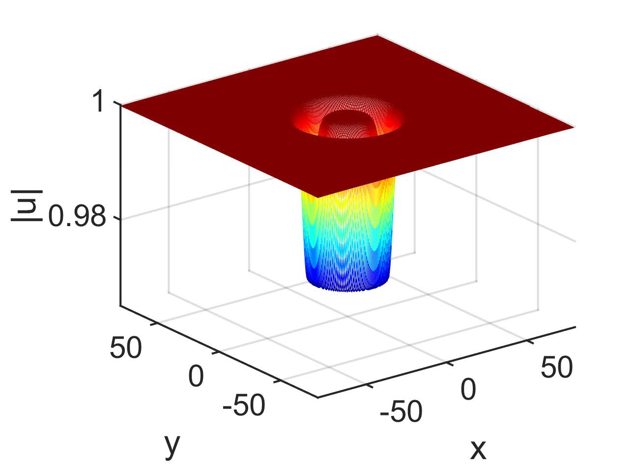
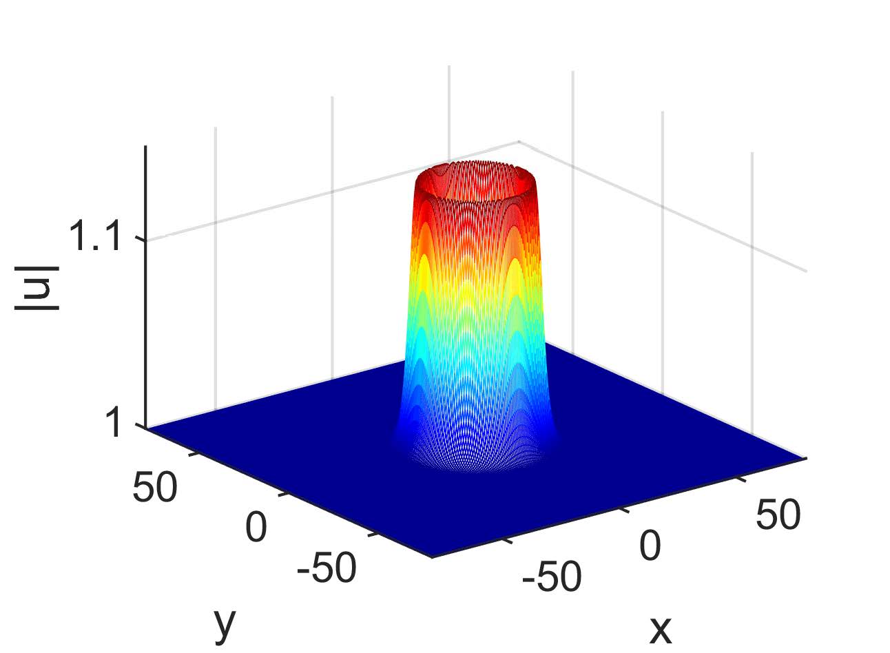
Figure 1: (Color Online) Typical RDS (top) and RAS (bottom), for $u_{0}=\alpha=1$ and $\nu=1$ ($\nu=1/3$) for the RAS (RDS).

Next, solve (11)-(12) for $\rho_{4}$ and substitute above to obtain the following nonlinear evolution equation for $\rho_{2}$:

$$\frac{\partial}{\partial R}\left(\frac{\partial\rho_{2}}{\partial Z}+\frac{3C}{2}\rho_{2}\frac{\partial\rho_{2}}{\partial R}+\frac{SC}{8}\frac{\partial^{3}\rho_{2}}{\partial R^{3}}+\frac{1}{2Z}\rho_{2}\right)+\frac{1}{2CZ^{2}}\frac{\partial^{2}\rho_{2}}{\partial\Theta^{2}}=0,$$ (13)

where parameter $S$ is given by:

$$S=\frac{2C^{2}\nu-1}{C^{2}}=\frac{4u_{0}^{2}\nu-1}{2u_{0}^{2}}.$$

Equation (13) is a cylindrical Kadomtsev-Petviashvili (cKP) equation, also known as Johnson’s equation, first introduced in the context of shallow water waves Johnson (1980). There exist transformations Klein et al. (2007) linking this model with the more commonly known KP equation in the Cartesian geometry Ablowitz and Segur (1981), which allows for construction of solutions of cKP from solutions of KP. Although —obviously— there exist other choices, here we focus on solutions with radial symmetry, which do not depend on $\Theta$. In this case, the system reduces to the cylindrical Korteweg-de Vries (cKdV) equation, which possesses cylindrical, sech²-shaped soliton solutions, on top of a rational background Hirota (1979):

$$\rho_{2}(R,Z)=\frac{R}{3CZ}+\frac{S\alpha^{2}}{Z}\mathrm{sech}^{2}\left(\frac{SC\alpha^{3}}{\sqrt{Z}}+\frac{\alpha R}{\sqrt{Z}}+R_{0}\right),$$ (14)

where, $\alpha$ is an arbitrary real parameter [of order $O(1)$]. Note that the characteristics of the solitons’ core, i.e., amplitude, power, velocity, and inverse width, scale as: $\alpha^{2}$, $\alpha^{4}$, $\alpha^{2}$, and $\alpha$, respectively, similarly to the case of the usual KdV solitons Ablowitz and Segur (1981).

Clearly, the sign of parameter $S$ determines the nature of the soliton: if $S<0$, the solitons are depressions off of the cw background and are, hence, dark solitons; if $S>0$, the solitons are humps on top of the cw background and are, thus, anti-dark solitons (note that if $S\rightarrow 0$, modification of the asymptotic analysis and inclusion of higher-order terms is needed as, e.g., in the shallow water wave problem Burde and Sergyeyev (2013)). Examples of these RDS and RAS solutions, as introduced above, are shown in Fig. 1. Notice that, having determined the form of the soliton [(14)], the refractive index can readily be found in terms of $\rho_{2}$: in fact, up to $O(\epsilon^{2})$, it is given by $n=n_{b}w\approx u_{0}^{2}(1+2\epsilon^{2}\rho_{2})$, thus having the form of an annular well (barrier) for the RDS (RAS).

Here, recalling that $\nu$ defines the degree of nonlocality, it is important to observe that $S<0\Rightarrow\nu<(1/2u_{0})^{2}$, while $S>0\Rightarrow\nu>(1/2u_{0})^{2}$. These inequalities indicate that RDS (RAS) are supported in a regime of weak (strong) nonlocality, as defined by the sign of $S$. Indeed, in the local limit with $\nu=0$ the NLS does not exhibit these RASs.

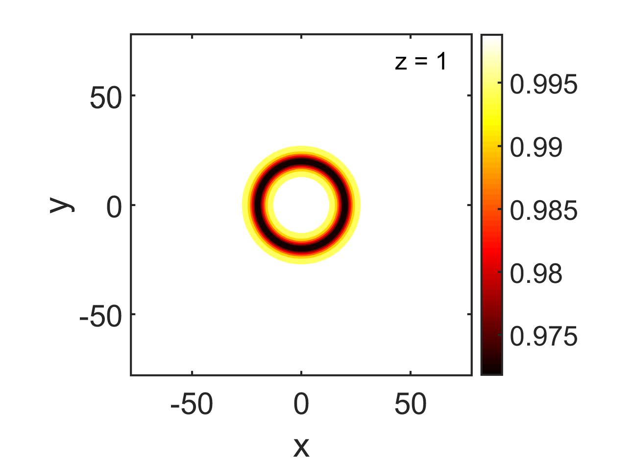
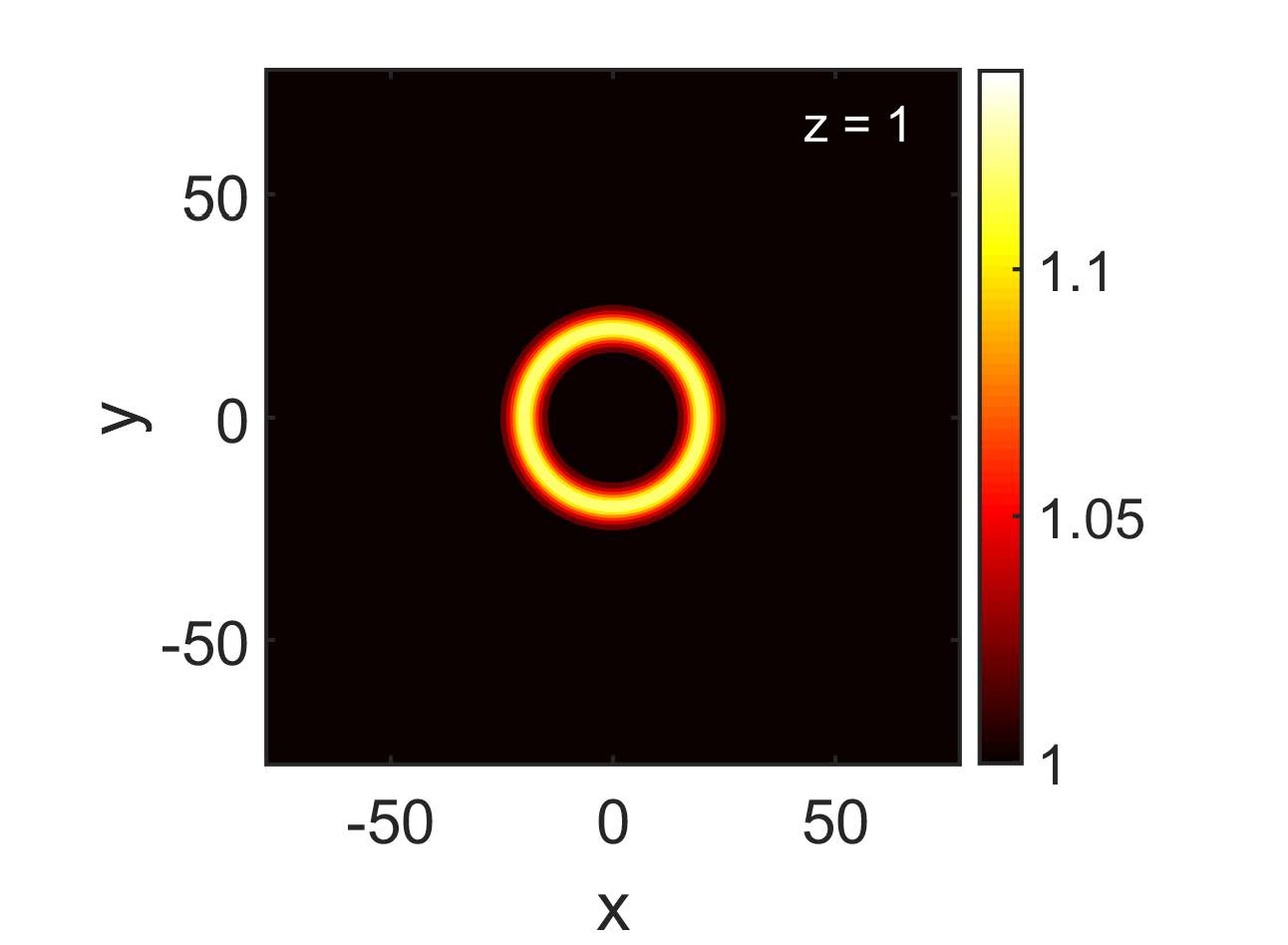
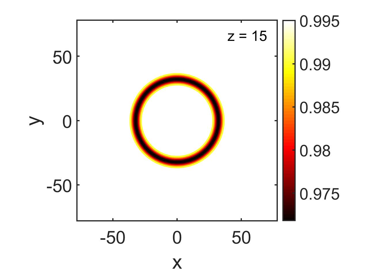
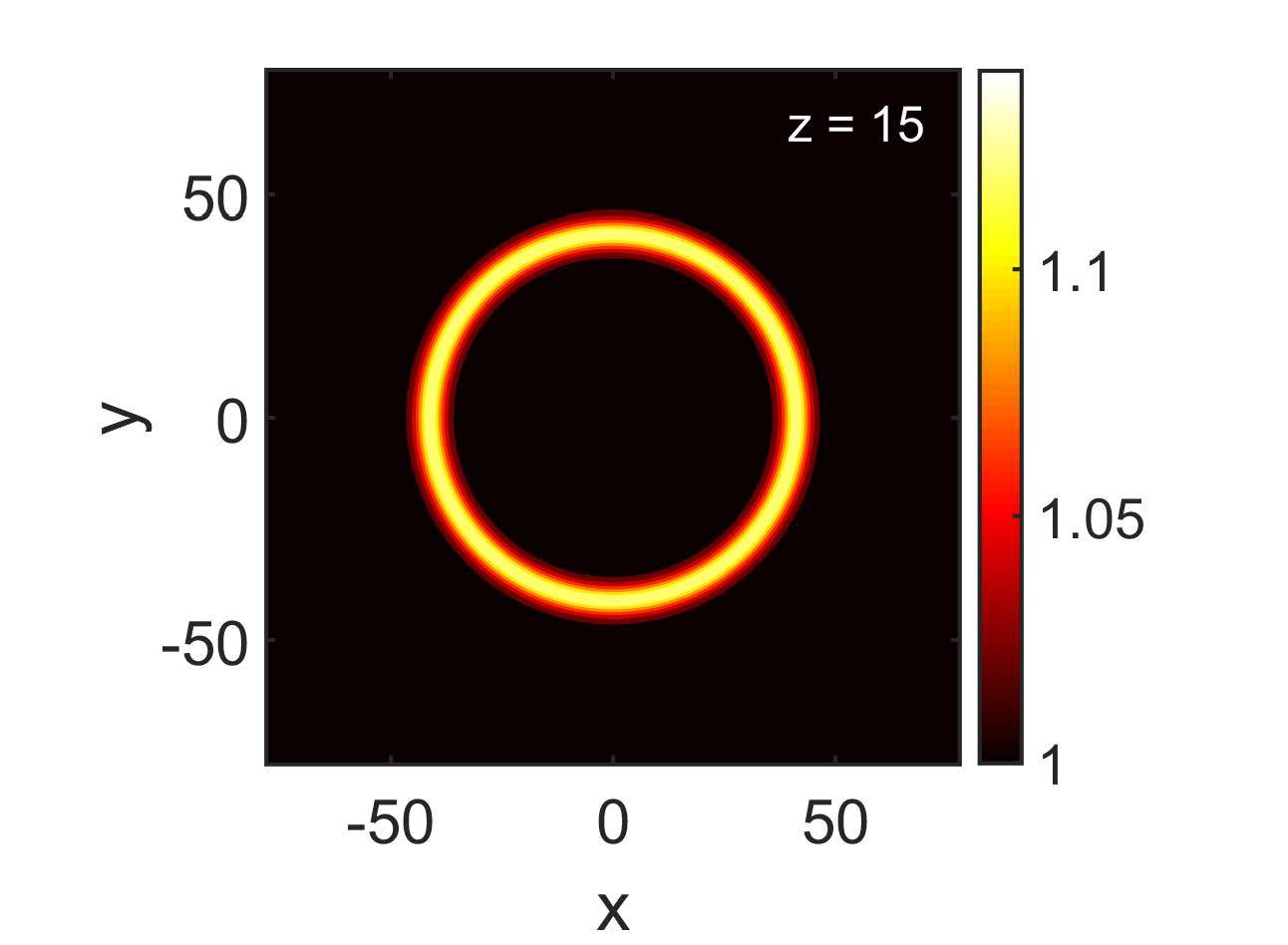
Figure 2: (Color Online) Evolution of a RDS (left) and a RAS (right). Parameter values are as in Fig. 1.

To numerically investigate the propagation properties of RDS and RAS, we evolve an initial ($z=1$) profile for both cases. Note that the rational background is not shown in Cartesian coordinates —see Ref. Santini (1980) for a discussion on the asymptotics for $z\rightarrow 0$. In Fig. 2, we evolve this initial condition under (1) for $u_{0}=\alpha=1$ and $\nu=1$ ($\nu=1/3$) for the RAS (RDS); note that in the simulations we use a high accuracy spectral integrator in Cartesian coordinates. We find that the role of nonlinearity is crucial for the soliton formation: indeed, in the linear regime, the electric field envelope features a diffraction-induced broadening, while when nonlinearity is present a strong localization is observed (results not shown here), and solitons are formed. Other interesting features, directly connected with the soliton form, (14), are reported below.

First, the two solitons propagate undistorted, i.e., the initial rings expand outwards, keeping their shapes during the evolution – at least for relatively short propagation distances. This fact, however, does not ensure stability of solitons, especially against azimuthal perturbations. Nevertheless, information regarding the RDS and RAS stability can be inferred from the cKP: in fact, (13) includes both models, so-called Klein et al. (2007) cKP-I (for $S<0$) and cKP-II (for $S>0$). Then, similarly to the case of the KP equation, where lower-dimensional line (KdV-type) solitons of KP-I (KP-II) are unstable (stable) against transverse perturbations Ablowitz and Segur (1981), we can infer the following: ring (cKdV-type) solitons of cKP-I (cKP-II), i.e., the RDS (for $S<0$) and RAS (for $S>0$) respectively, are unstable (stable) against azimuthal perturbations. Nevertheless, in our simulations we have not observed the instability of RDS, for propagation distances up to $z\approx 70$.

Second, we find that the soliton velocities are $C=\sqrt{2/3}$ for the RDS and $C=\sqrt{2}$ for the RAS, with a deviation less than $2\%$ from the analytical prediction. It is also observed in Fig. 2 that, indeed, the RAS’s radius is larger than that of RDS at the same propagation distance. Note that the amplitudes of RDS and RAS depend on $S$, but do not depend on $C$ (the sign of $C$ determines if the soliton will contract inwards or expand outwards). Thus, according to these results, the RDS and the RAS cannot coexist. However, we note that in the presence of a competing quintic nonlinearity, it would be in principle possible to find parameter regimes where RDS and RAS do coexist, as was the case in Refs. Crosta et al. (2011); Zhou et al. (2011) (see also Refs. Kivshar (1991); Kivshar and Afanasjev (1991); Nistazakis et al. (2001b) for the same effect in a setting incorporating third-order dispersion).

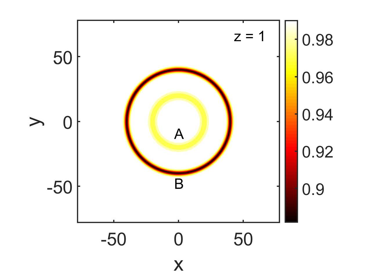
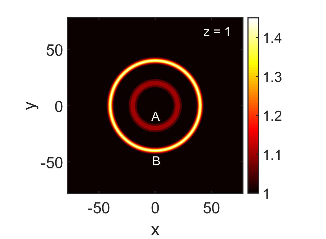
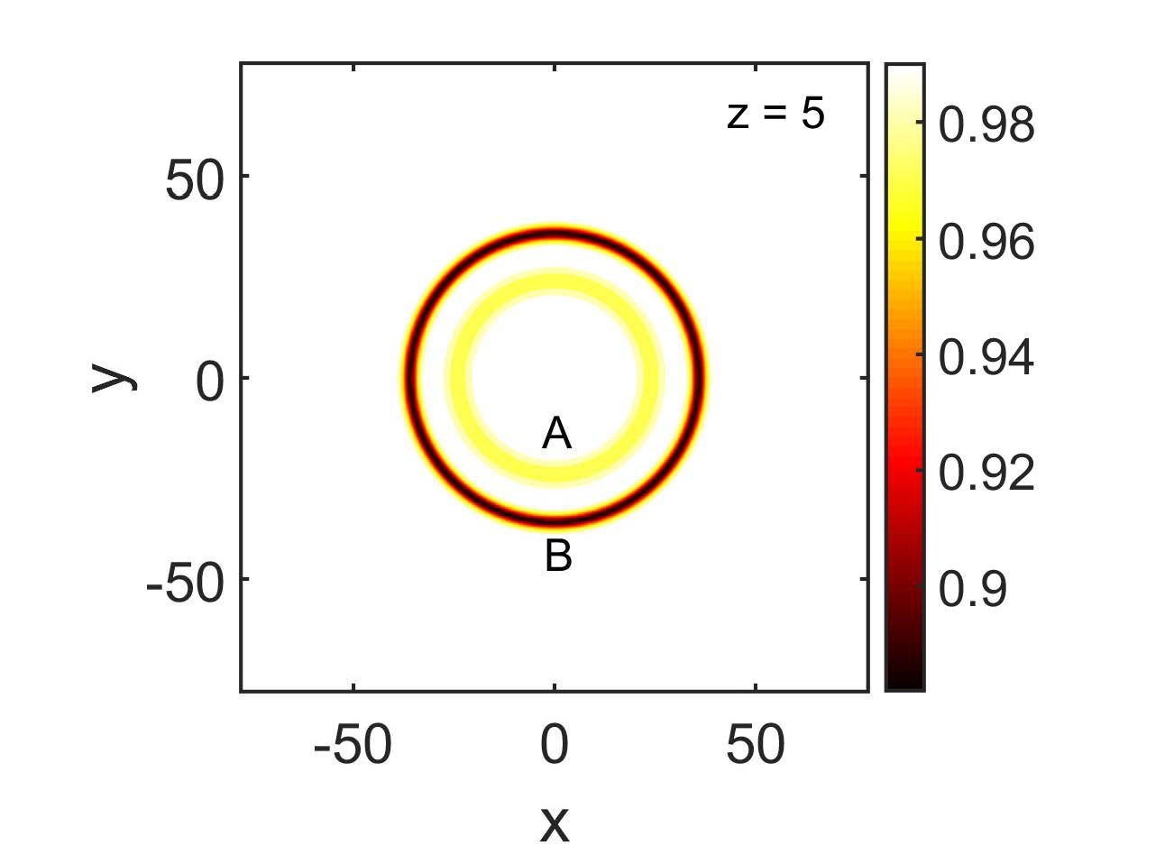
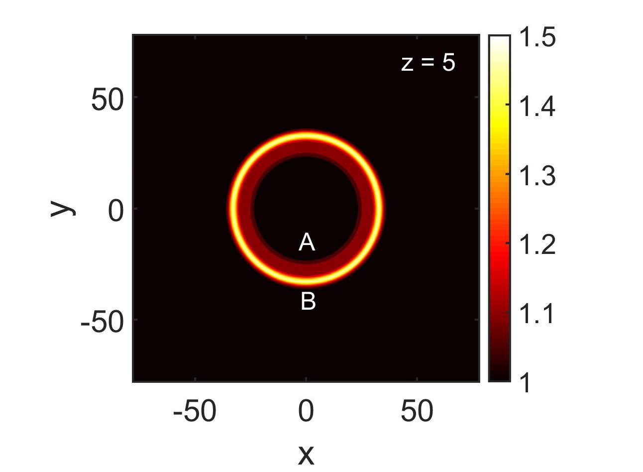
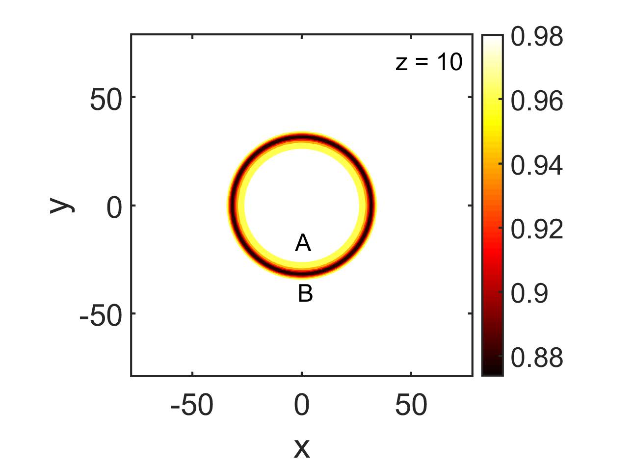
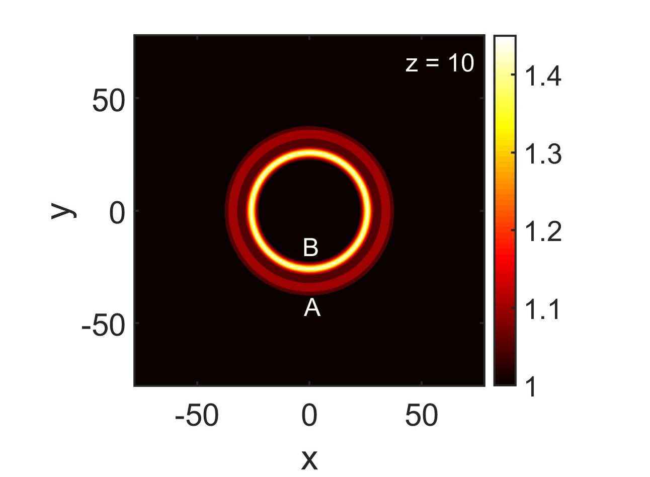
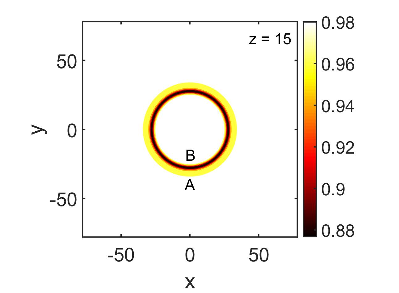
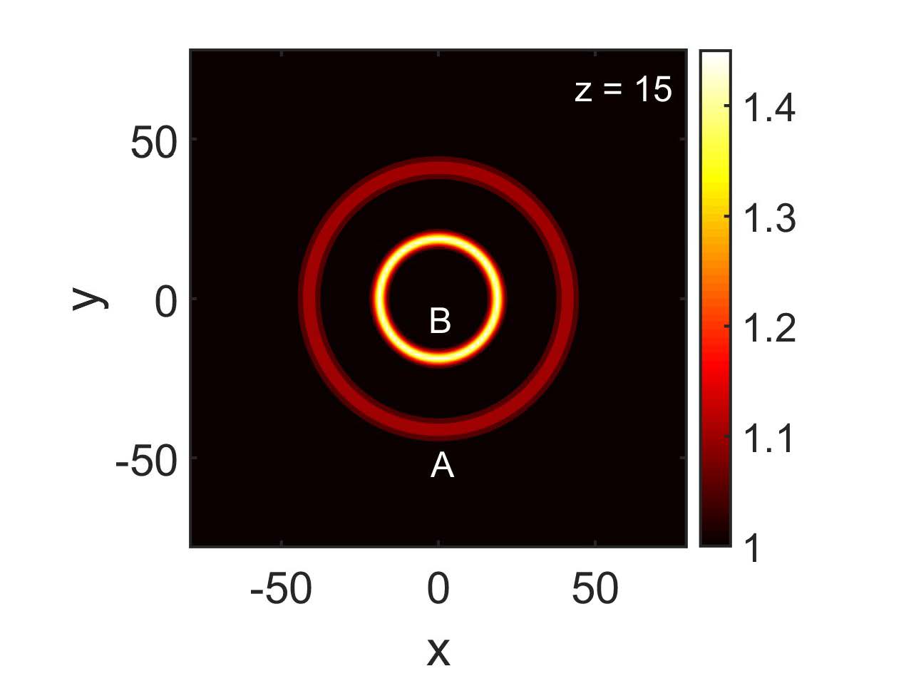
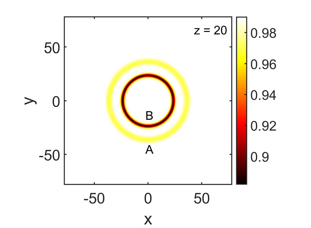
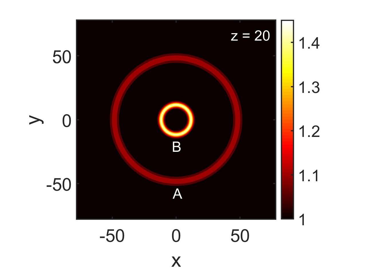
Figure 3: (Color Online) Interaction of RDSs (left) and RNAs (right) solitons.

Third, although RDS and the RAS cannot coexist and, thus, cannot interact with each other, it is possible to study interactions of two solitons of the same type, namely RDS-RDS or RAS-RAS: this would be an important test on their robustness and solitonic character —at least up to relatively short propagation distances, as explained above. In Fig. 3, we show the interaction of two solitons of unequal amplitudes, namely $\alpha=1$ ($\alpha=2$) for the inner (outer) soliton; other parameters are as above. The velocities are also chosen as before, but with a different sign, so that the solitons will undergo a head-on collision. As seen, the collision is quasielastic: after passing through each other, the solitons restore their shapes. This behavior is in agreement with the perturbation theory of Ref. Nistazakis et al. (2001a), which predicts that the head-on collision is elastic up to the second-order.

It should be mentioned that the numerical results obtained above refer to the collision between concentric RDS or RAS. However, there exists the possibility of the collision between slightly mismatched rings. In this case, it is expected that the collision will produce small oscillations of the rings, that will be oscillating between two elliptic configurations with small positive and negative eccentricities.

To conclude, we have found and analyzed ring dark solitons (RDSs) and ring anti-dark solitons (RASs) in nonlocal media. These structures were found as special, radially symmetric, solutions of a cylindrical KdV model, which is a lower-dimensional reduction of an underlying cylindrical KP (alias Johnson’s) equation. RDSs and RASs are supported, respectively, in a weak or strong nonlocal regime, as defined by the sign of a characteristic parameter. The same parameter controls the stability of these structures: in particular, RDSs (RASs) are predicted to be unstable (stable) against azimuthal perturbations. These facts highlight the role of nonlocality, which, not only support RASs that do not exist in the local limit, but also renders them stable in the higher-dimensional setting. For relatively short propagation distances, both structures were found to propagate undistorted and remain unaffected even under head-on collisions; this attests to their solitonic character. Importantly, even for longer propagation distances, instabilities were not observed in our simulations. This suggests that RDSs and RASs have a good chance to be observed in experiments.

References

- Kivshar and Luther-Davies (1998) Y. S. Kivshar and B. Luther-Davies, Phys. Rep. 298, 81 (1998).
- Kuznetsov and Turitsyn (1998) E. A. Kuznetsov and S. K. Turitsyn, JETP 67, 1583 (1998).
- Tikhonenko et al. (1996) V. Tikhonenko, J. Christou, B. LutherDavies, and Y. S. Kivshar, Opt. Lett. 21, 1129 (1996).
- Kivshar and Yang (1994) Y. S. Kivshar and X. Yang, Phys. Rev. E 50, R40 (1994).
- Frantzeskakis and Malomed (1999) D. J. Frantzeskakis and B. A. Malomed, Phys. Lett. A 264, 179 (1999).
- Nistazakis et al. (2001a) H. E. Nistazakis, D. J. Frantzeskakis, B. A. Malomed, and P. G. Kevrekidis, Phys. Lett. A 285, 157 (2001a).
- Dreischuh et al. (2002) A. Dreischuh, D. Neshev, G. G. Paulus, F. Grasbon, and H. Walther, Phys. Rev. E 66, 066611 (2002).
- Dreischuh et al. (1996) A. Dreischuh, V. Kamenov, and S. Dinev, Appl. Phys. B 63, 145 (1996).
- Theocharis et al. (2003) G. Theocharis, D. J. Frantzeskakis, P. G. Kevrekidis, B. A. Malomed, and Y. S. Kivshar, Phys. Rev. Lett. 90, 120403 (2003).
- Rodrigues et al. (2014) A. S. Rodrigues, P. G. Kevrekidis, R. Carretero-González, J. Cuevas-Maraver, D. J. Frantzeskakis, and F. Palmero, J. Phys.: Cond. Mat. 26, 155801 (2014).
- Dominici et al. (2013) L. Dominici, D. Ballarini, M. D. Giorgi, E. Cancellieri, B. S. Fernández, A. Bramati, G. Gigli, F. Laussy, and D. Sanvitto, arXiv p. 1309.3083 (2013).
- Krolikowski et al. (2004) W. Krolikowski, O. Bang, N. I. Nikolov, D. Neshev, J. Wyller, J. J. Rasmussen, and D. Edmundson, J. Opt. B: Quantum Semiclass. Opt. 6, S288 (2004).
- Alberucci et al. (2014) A. Alberucci, G. Assanto, J. M. L. MacNeil, and N. F. Smyth, J. Nonlinear Optic. Phys. Mat. 23, 1450046 (2014).
- Kartashov and Torner (2007) Y. V. Kartashov and L. Torner, Opt. Lett. 32, 946–948 (2007).
- Kong et al. (2010) Q. Kong, Q. Wang, O. Bang, and W. Królikowski, Opt. Lett. 35, 2152–2154 (2010).
- Piccardi et al. (2011) A. Piccardi, A. Alberucci, N. Tabiryan, and G. Assanto, Opt. Lett. 36, 1356 (2011).
- Assanto et al. (2011) G. Assanto, T. R. Marchant, A. A. Minzoni, and N. F. Smyth, Phys. Rev. E 84, 066602 (2011).
- Pu et al. (2012) S. Pu, C. Hou, K. Zhan, and C. Yuan, Physica Scr. 85, 015402 (2012).
- Horikis (2015) T. P. Horikis, J. Phys. A: Math. Theor. 48, 02FT01 (2015).
- Armaroli et al. (2009) A. Armaroli, S. Trillo, and A. Fratalocchi, Phys. Rev. A 80, 053803 (2009).
- Ghofraniha et al. (2007) N. Ghofraniha, C. Conti, G. Ruocco, and S. Trillo, Phys. Rev. Lett. 99, 043903 (2007).
- Assanto et al. (2008) G. Assanto, T. R. Marchant, and N. F. Smyth, Phys. Rev. A 78, 063808 (2008).
- Xu et al. (2015) G. Xu, D. Vocke, D. Faccio, J. Garnier, T. Roger, S. Trillo, and A. Picozzi, Nature Comm. 6, 8131 (2015).
- Assanto (2012) G. Assanto, Nematicons: Spatial Optical Solitons in Nematic Liquid Crystals (Wiley-Blackwell, 2012).
- Królikowski and Bang (2000) W. Królikowski and O. Bang, Phys. Rev. E 63, 016610 (2000).
- Peccianti and Assanto (2012) M. Peccianti and G. Assanto, Phys. Rep. 516, 147 (2012).
- Alberucci and Assanto (2013) A. Alberucci and G. Assanto, Mol. Cryst. Liq. Cryst. 572, 2 (2013).
- Assanto et al. (2009) G. Assanto, A. A. Minzoni, and N. F. Smyth, J. Nonlinear Opt. Phys. Mater. 18, 657 (2009).
- Sciberras et al. (2014) L. W. Sciberras, A. A. Minzoni, N. F. Smyth, and G. Assanto, J. Nonlinear Optic. Phys. Mat. 23, 1450045 (2014).
- Johnson (1980) R. S. Johnson, J. Fluid Mech. 97, 701 (1980).
- Reinbert et al. (2006) C. G. Reinbert, A. A. Minzoni, and N. F. Smyth, J. Opt. Soc. Am. B 23, 294 (2006).
- Horikis and Frantzeskakis (2014) T. P. Horikis and D. J. Frantzeskakis, Rom. J. Phys. 59, 195 (2014).
- Krolikowski et al. (2001) W. Krolikowski, O. Bang, J. J. Rasmussen, and J. Wyller, Phys. Rev. E 64, 016612 (2001).
- Klein et al. (2007) C. Klein, V. B. Matveev, and A. O. Smirnov, Theor. Math. Phys. 152, 1132 (2007).
- Ablowitz and Segur (1981) M. J. Ablowitz and H. Segur, Solitons and the Inverse Scattering Transform (SIAM Studies in Applied Mathematics, 1981).
- Hirota (1979) R. Hirota, Phys. Lett. 71A, 393 (1979).
- Burde and Sergyeyev (2013) G. I. Burde and A. Sergyeyev, J. Phys. A: Math. Theor. 46, 075501 (2013).
- Santini (1980) P. Santini, Il Nuovo Cimento 57A, 387 (1980).
- Crosta et al. (2011) M. Crosta, A. Fratalocchi, and S. Trillo, Phys. Rev. A 84, 063809 (2011).
- Zhou et al. (2011) Z. Zhou, Y. Du, C. Hou, H. Tian, and Y. Wang, J. Opt. Soc. Am. B 28, 1583 (2011).
- Kivshar (1991) Y. S. Kivshar, Opt. Lett. 16, 892 (1991).
- Kivshar and Afanasjev (1991) Y. S. Kivshar and V. V. Afanasjev, Phys. Rev. A 44, R1446 (1991).
- Nistazakis et al. (2001b) H. E. Nistazakis, D. J. Frantzeskakis, and B. A. Malomed, Phys. Rev. E 64, 026604 (2001b).