On the wave equation with hyperbolic dynamical boundary conditions, interior and boundary damping and supercritical sources

Abstract.

The aim of this paper is to study the problem

$$\begin{cases}u_{tt}-\Delta u+P(x,u_{t})=f(x,u)\qquad&\text{in $(0,\infty)\times\Omega$,}\\ u=0&\text{on $(0,\infty)\times\Gamma_{0}$,}\\ u_{tt}+\partial_{\nu}u-\Delta_{\Gamma}u+Q(x,u_{t})=g(x,u)\qquad&\text{on $(0,\infty)\times\Gamma_{1}$,}\\ u(0,x)=u_{0}(x),\quad u_{t}(0,x)=u_{1}(x)&\text{in $\overline{\Omega}$,}\end{cases}$$

where $\Omega$ is a bounded open subset of $\mathbb{R}^{N}$ with $C^{1}$ boundary ($N\geq 2$), $\Gamma=\partial\Omega$, $\Gamma_{1}$ is relatively open on $\Gamma$, $\Delta_{\Gamma}$ denotes the Laplace–Beltrami operator on $\Gamma$, $\nu$ is the outward normal to $\Omega$, and the terms $P$ and $Q$ represent nonlinear damping terms, while $f$ and $g$ are nonlinear perturbations.

In the paper we establish local and global existence, uniqueness and Hadamard well–posedness results when source terms can be supercritical or super-supercritical.

1. Introduction and main results

1.1. Presentation of the problem and literature overview

We deal with the evolution problem consisting of the wave equation posed in a bounded regular open subset of $\mathbb{R}^{N}$, supplied with a second order dynamical boundary condition of hyperbolic type, in presence of interior and/or boundary damping terms and sources. More precisely we consider the initial –and–boundary value problem

(1.1) $$\begin{cases}u_{tt}-\Delta u+P(x,u_{t})=f(x,u)\qquad&\text{in $(0,\infty)\times\Omega$,}\\ u=0&\text{on $(0,\infty)\times\Gamma_{0}$,}\\ u_{tt}+\partial_{\nu}u-\Delta_{\Gamma}u+Q(x,u_{t})=g(x,u)\qquad&\text{on $(0,\infty)\times\Gamma_{1}$,}\\ u(0,x)=u_{0}(x),\quad u_{t}(0,x)=u_{1}(x)&\text{in $\overline{\Omega}$,}\end{cases}$$

where $\Omega$ is a bounded open subset of $\mathbb{R}^{N}$ ($N\geq 2$) with $C^{1}$ boundary (see [31]). We denote $\Gamma=\partial\Omega$ and we assume $\Gamma=\Gamma_{0}\cup\Gamma_{1}$, $\Gamma_{0}\cap\Gamma_{1}=\emptyset$, $\Gamma_{1}$ being relatively open on $\Gamma$ (or equivalently $\overline{\Gamma_{0}}=\Gamma_{0}$). Moreover, denoting by $\sigma$ the standard Lebesgue hypersurface measure on $\Gamma$, we assume that $\sigma(\overline{\Gamma}_{0}\cap\overline{\Gamma}_{1})=0$. These properties of $\Omega$, $\Gamma_{0}$ and $\Gamma_{1}$ will be assumed, without further comments, throughout the paper. Moreover $u=u(t,x)$, $t\geq 0$, $x\in\Omega$, $\Delta=\Delta_{x}$ denotes the Laplace operator with respect to the space variable, while $\Delta_{\Gamma}$ denotes the Laplace–Beltrami operator on $\Gamma$ and $\nu$ is the outward normal to $\Omega$.

The terms $P$ and $Q$ represent nonlinear damping terms, i.e. $P(x,v)v\geq 0$, $Q(x,v)v\geq 0$, the cases $P\equiv 0$ and $Q\equiv 0$ being specifically allowed, while $f$ and $g$ represent nonlinear source, or sink, terms. The specific assumptions on them will be introduced later on.

Problems with kinetic boundary conditions, that is boundary conditions involving $u_{tt}$ on $\Gamma$, or on a part of it, naturally arise in several physical applications. A one dimensional model was studied by several authors to describe transversal small oscillations of an elastic rod with a tip mass on one endpoint, while the other one is pinched. See [3, 17, 18, 32, 38, 37, 41] and also [40] were a piezoelectric stack actuator is modeled.

A two dimensional model introduced in [28] deals with a vibrating membrane of surface density $\mu$, subject to a tension $T$, both taken constant and normalized here for simplicity. If $u(t,x)$, $x\in\Omega\subset\mathbb{R}^{2}$ denotes the vertical displacement from the rest state, then (after a standard linear approximation) $u$ satisfies the wave equation $u_{tt}-\Delta u=0$, $(t,x)\in\mathbb{R}\times\Omega$. Now suppose that a part $\Gamma_{0}$ of the boundary is pinched, while the other part $\Gamma_{1}$ carries a constant linear mass density $m>0$ and it is subject to a linear tension $\tau$. A practical example of this situation is given by a drumhead with a hole in the interior having a thick border, as common in bass drums. One linearly approximates the force exerted by the membrane on the boundary with $-\partial_{\nu}u$. The boundary condition thus reads as $mu_{tt}+\partial_{\nu}u-\tau\Delta_{\Gamma_{1}}u=0$. In the quoted paper the case $\Gamma_{0}=\emptyset$ and $\tau=0$ was studied, while here we consider the more realistic case $\Gamma_{0}\not=\emptyset$ and $\tau>0$, with $\tau$ and $m$ normalized for simplicity. We would like to mention that this model belongs to a more general class of models of Lagrangian type involving boundary energies, as introduced for example in [23].

A three dimensional model involving kinetic dynamical boundary conditions comes out from [26], where a gas undergoing small irrotational perturbations from rest in a domain $\Omega\subset\mathbb{R}^{3}$ is considered. Normalizing the constant speed of propagation, the velocity potential $\phi$ of the gas (i.e. $-\nabla\phi$ is the particle velocity) satisfies the wave equation $\phi_{tt}-\Delta\phi=0$ in $\mathbb{R}\times\Omega$. Each point $x\in\partial\Omega$ is assumed to react to the excess pressure of the acoustic wave like a resistive harmonic oscillator or spring, that is the boundary is assumed to be locally reacting (see [42, pp. 259–264]). The normal displacement $\delta$ of the boundary into the domain then satisfies $m\delta_{tt}+d\delta_{t}+k\delta+\rho\phi_{t}=0$, where $\rho>0$ is the fluid density and $m,d,k\in C(\partial\Omega)$, $m,k>0$, $d\geq 0$. When the boundary is nonporous one has $\delta_{t}=\partial_{\nu}\phi$ on $\mathbb{R}\times\partial\Omega$, so the boundary condition reads as $m\delta_{tt}+d\partial_{\nu}\phi+k\delta+\rho\phi_{t}=0$. In the particular case $m=k$ and $d=\rho$ (see [26, Theorem 2]) one proves that $\phi_{|\Gamma}=\delta$, so the boundary condition reads as $m\phi_{tt}+d\partial_{\nu}\phi+k\phi+\rho\phi_{t}=0$, on $\mathbb{R}\times\partial\Omega$. Now, if one consider the case in which the boundary is not locally reacting, as in [9], one adds a Laplace–Beltrami term so getting a dynamical boundary condition like in (1.1).

Several papers in the literature deal with the wave equation with kinetic boundary conditions. This fact is even more evident if one takes into account that, plugging the equation in (1.1) into the boundary condition, we can rewrite it as $\Delta u+\partial_{\nu}u-\Delta_{\Gamma}u+Q(x,u_{t})+P(x,u_{t})=f(x,u)+g(x,u)$. Such a condition is usually called a generalized Wentzell boundary condition, at least when nonlinear perturbations are not present. We refer to [43], where abstract semigroup techniques are applied to dissipative wave equations, and to [21, 22, 51, 56, 57, 59].

Here we shall consider this type of kinetic boundary condition in connection with nonlinear boundary damping and source terms. These terms have been considered by several authors, but mainly in connection with first order dynamical boundary conditions. See [4, 5, 10, 11, 12, 14, 15, 16, 24, 35, 53, 60]. The competition between interior damping and source terms is methodologically related to the competition between boundary damping and source and it possesses a large literature as well. See [6, 27, 36, 44, 45, 46, 52].

A linear problem strongly related to (1.1) has also been recently studied in [25, 30], and another one in the recent paper [58], dealing with holography, a main theme in theoretical high energy physics and quantum gravity. See also [29].

Problem (1.1) has been studied by the author in the recent paper [55] (see also [54]) when source/sink terms are subcritical, that is when the Nemitskii operators associated to $f$ and $g$ are locally Lischitz, respectively from $H^{1}(\Omega)$ to $L^{2}(\Omega)$ and from $H^{1}(\Gamma)$ to $L^{2}(\Gamma)$. In particular, using nonlinear semigroup theory, local Hadamard well–posedness, and hence also local existence and uniqueness, has been established in the natural energy space related to the problem. Moreover global existence and well–posedness have been proved when source terms are either sublinear or dominated by corresponding damping terms.

The aim of the present paper is to extend the results of [55] to possibly non–subcritical perturbation terms $f$ and $g$. As a consequence we do not expect to get new results when all perturbation terms are subcritical, as in the case $N=2$, but we want to cover the case when one term is subcritical while the other one is non–subcritical. As a byproduct the results in [55] will be a subcase of the more general analysis presented in the sequel.

Our main motivation is constituted by the three dimensional case, in which only the term $f$ can be non–subcritical. Hence our choice to consider also non–subcritical boundary terms $g$ is only of mathematical interest, but it is motivated as follows. At first in dimensions higher than $3$ both terms can be non–subcritical. At second this extension is costless, since all estimates used in the paper will be explicitly proved only for $f$ (in relation with $P$) and then trivially transposed to $g$. Finally to consider terms $f$ and $g$ under the same setting allows to give results in which $f$ and $g$ play a symmetric role, as they do in dimension $N=4$.

1.2. A simplified problem, source classification and main assumptions

To best illustrate our results we shall consider, in this section, the following simplified version of problem (1.1)

(1.2) $$\begin{cases}u_{tt}-\Delta u+\alpha(x)P_{0}(u_{t})=f_{0}(u)\qquad&\text{in $(0,\infty)\times\Omega$,}\\ u=0&\text{on $(0,\infty)\times\Gamma_{0}$,}\\ u_{tt}+\partial_{\nu}u-\Delta_{\Gamma}u+\beta(x)Q_{0}(u_{t})=g_{0}(u)\qquad&\text{on $(0,\infty)\times\Gamma_{1}$,}\\ u(0,x)=u_{0}(x),\quad u_{t}(0,x)=u_{1}(x)&\text{in $\overline{\Omega}$,}\end{cases}$$

where $\alpha\in L^{\infty}(\Omega)$, $\beta\in L^{\infty}(\Gamma_{1})$, $\alpha,\beta\geq 0$, and the following assumptions hold:

1. $P_{0}$ and $Q_{0}$ are continuous and monotone increasing in $\mathbb{R}$, $P_{0}(0)=Q_{0}(0)=0$, and there are $m,\mu>1$ such that

   $$0<\varliminf_{|v|\to\infty}\frac{|P_{0}(v)|}{|v|^{m-1}}\leq\varlimsup_{|v|\to\infty}\frac{|P_{0}(v)|}{|v|^{m-1}}<\infty,\quad\varliminf_{|v|\to 0}\frac{|P_{0}(v)|}{|v|^{m-1}}>0,$$

   $$0<\varliminf_{|v|\to\infty}\frac{|Q_{0}(v)|}{|v|^{\mu-1}}\leq\varlimsup_{|v|\to\infty}\frac{|Q_{0}(v)|}{|v|^{\mu-1}}<\infty,\quad\varliminf_{|v|\to 0}\frac{|Q_{0}(v)|}{|v|^{\mu-1}}>0;$$

2. $f_{0},g_{0}\in C^{0,1}_{\text{loc}}(\mathbb{R})$ and there are exponents $p,q\geq 2$ such that

   $$|f_{0}^{\prime}(u)|=O(|u|^{p-2})\qquad\text{and}\quad|g_{0}^{\prime}(u)|=O(|u|^{q-2})\quad\text{as $|u|\to\infty$.}$$

Our model nonlinearities, trivially satisfying assumptions (I–II), are given by

(1.3) $$\left\{\begin{aligned} P_{0}(v)=&P_{1}(v):=a|v|^{\widetilde{m}-2}v+|v|^{m-2}v,\quad&&1<\widetilde{m}\leq m,\quad&&a\geq 0,\\ Q_{0}(v)=&Q_{1}(v):=b|v|^{\widetilde{\mu}-2}v+|v|^{\mu-2}v,\quad&&1<\widetilde{\mu}\leq\mu,\quad&&b\geq 0,\\ f_{0}(u)=&f_{1}(u):=\widetilde{\gamma}|u|^{\widetilde{p}-2}u+\gamma|u|^{p-2}u+c_{1},\quad&&2\leq\widetilde{p}\leq p,\quad&&\widetilde{\gamma},\gamma,c_{1}\in\mathbb{R},\\ g_{0}(u)=&g_{1}(u):=\widetilde{\delta}|u|^{\widetilde{q}-2}u+\delta|u|^{q-2}u+c_{2},\,\quad&&2\leq\widetilde{q}\leq q,\quad&&\widetilde{\delta},\delta,c_{2}\in\mathbb{R}.\end{aligned}\right.$$

We introduce the critical exponents ${r_{\phantom{a}\!\!\!\!{}_{\Omega}}}$ and ${r_{\phantom{a}\!\!\!\!{}_{\Gamma}}}$ of the Sobolev embeddings of $H^{1}(\Omega)$ and $H^{1}(\Gamma)$ into the corresponding Lebesgue spaces, that is

$${r_{\phantom{a}\!\!\!\!{}_{\Omega}}}=\begin{cases}\dfrac{2N}{N-2}&\text{if $N\geq 3$,}\\ \infty&\text{if $N=2$},\end{cases}\qquad{r_{\phantom{a}\!\!\!\!{}_{\Gamma}}}=\begin{cases}\dfrac{2(N-1)}{N-3}&\text{if $N\geq 4$,}\\ \infty&\text{if $N=2,3$}.\end{cases}$$

The term $f_{0}$, or $f_{1}$, is usually classified as follows in the literature (see [11, 12]):

1. $f_{0}$ is subcritical if $2\leq p\leq 1+{r_{\phantom{a}\!\!\!\!{}_{\Omega}}}/2$, when the Nemitskii operator $\widehat{f_{0}}$ associated to $f_{0}$ is locally Lipschitz from $H^{1}(\Omega)$ into $L^{2}(\Omega)$;

2. $f_{0}$ is supercritical if $1+{r_{\phantom{a}\!\!\!\!{}_{\Omega}}}/2<p\leq{r_{\phantom{a}\!\!\!\!{}_{\Omega}}}$, when $\widehat{f_{0}}$ is no longer locally Lipschitz from $H^{1}(\Omega)$ into $L^{2}(\Omega)$ but it still possesses a potential energy in $H^{1}(\Omega)$;

3. $f_{0}$ is super–supercritical if $p>{r_{\phantom{a}\!\!\!\!{}_{\Omega}}}$, when $\widehat{f_{0}}$ has no potentials in $H^{1}(\Omega)$.

The analogous classification is made for $g_{0}$, depending on $q$ and ${r_{\phantom{a}\!\!\!\!{}_{\Gamma}}}$.

In [55] the case when (I–II) hold and $f_{0}$ and $g_{0}$ are both subcritical was studied, while here we are concerned with possibly supercritical and super–supercritical terms. To deal with them we need two further main assumptions:

1. $\operatorname{essinf}_{\Omega}\alpha>0$ when $p>1+{r_{\phantom{a}\!\!\!\!{}_{\Omega}}}/2$, $\operatorname{essinf}_{\Gamma_{1}}\beta>0$ when $q>1+{r_{\phantom{a}\!\!\!\!{}_{\Gamma}}}/2$, and

   (1.4) $$2\leq p\leq 1+{r_{\phantom{a}\!\!\!\!{}_{\Omega}}}/\overline{m}^{\prime},\quad 2\leq q\leq 1+{r_{\phantom{a}\!\!\!\!{}_{\Gamma}}}/\overline{\mu}^{\prime},$$

   where $\overline{m}=\max\{2,m\}$ and $\overline{\mu}=\max\{2,\mu\}$;

2. if $1+{r_{\phantom{a}\!\!\!\!{}_{\Omega}}}/2<p=1+{r_{\phantom{a}\!\!\!\!{}_{\Omega}}}/m^{\prime}$ then $N\leq 4$, $f_{0}\in C^{2}(\mathbb{R})$ and $\varlimsup\limits_{|u|\to\infty}\frac{|f_{0}^{\prime\prime}(u)|}{|u|^{p-3}}<\infty$;
   if $1+{r_{\phantom{a}\!\!\!\!{}_{\Gamma}}}/2<q=1+{r_{\phantom{a}\!\!\!\!{}_{\Gamma}}}/\mu^{\prime}$ then $N\leq 5$, $g_{0}\in C^{2}(\mathbb{R})$ and $\varlimsup\limits_{|u|\to\infty}\frac{|g_{0}^{\prime\prime}(u)|}{|u|^{q-3}}<\infty$.

Remark 1.1.

Clearly assumption (III) can be equally refereed to our model nonlinearities in (1.3), while they satisfy (IV) if

• $N\leq 4$ and $\widetilde{p}>3$ or $\widetilde{\gamma}=0$ provided $1+{r_{\phantom{a}\!\!\!\!{}_{\Omega}}}/2<p=1+{r_{\phantom{a}\!\!\!\!{}_{\Omega}}}/m^{\prime}$;

• $N\leq 5$ and $\widetilde{q}>3$ or $\widetilde{\delta}=0$ provided $1+{r_{\phantom{a}\!\!\!\!{}_{\Gamma}}}/2<q=1+{r_{\phantom{a}\!\!\!\!{}_{\Gamma}}}/\mu^{\prime}$.

Remark 1.2.

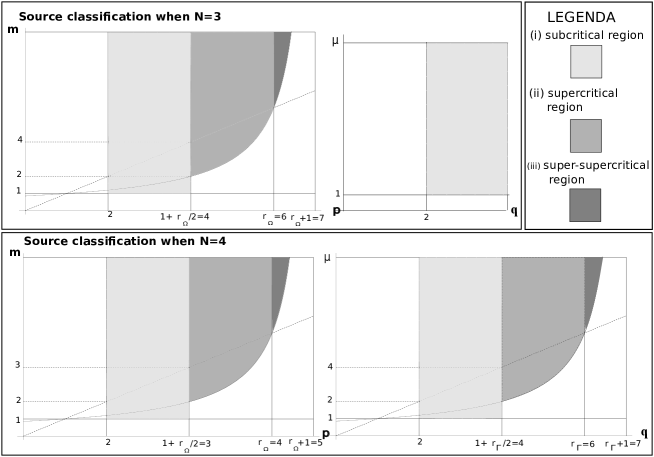
Figure 1. The regions covered by (1.4) in dimensions $N=3,4$.

The sets in the planes $(p,m)$ and $(q,\mu)$, for which (1.4) holds, corresponding to the classification above, are illustrated in dimensions $N=3,4$ in Figure 1. The subcritical regions were studied in [55], while this paper covers all regions in the picture. In dimensions $N=3$ and $N=4$, the first one being of physical relevance, (IV) is a mild strengthening of (II). When $N=5$ assumption (IV) excludes parameter couples for which $1+{r_{\phantom{a}\!\!\!\!{}_{\Omega}}}/2<p=1+{r_{\phantom{a}\!\!\!\!{}_{\Omega}}}/m^{\prime}$, while it is a strengthening of (II) for the term $g_{0}$. When $N\geq 6$ assumption (IV) simply excludes parameter couples for which $1+{r_{\phantom{a}\!\!\!\!{}_{\Omega}}}/2<p=1+{r_{\phantom{a}\!\!\!\!{}_{\Omega}}}/m^{\prime}$ and $1+{r_{\phantom{a}\!\!\!\!{}_{\Gamma}}}/2<q=1+{r_{\phantom{a}\!\!\!\!{}_{\Gamma}}}/\mu^{\prime}$.

To present our results it is useful to subclassify supercritical terms $f_{0}$, by distinguishing between intercritical ones, when $1+{r_{\phantom{a}\!\!\!\!{}_{\Omega}}}/2<p<{r_{\phantom{a}\!\!\!\!{}_{\Omega}}}$, and Sobolev critical ones when $p={r_{\phantom{a}\!\!\!\!{}_{\Omega}}}$. Moreover terms $f_{0}$ for which $p<1+{r_{\phantom{a}\!\!\!\!{}_{\Omega}}}/m^{\prime}$ when $m>2$ will be treated in a different way from those for which $p=1+{r_{\phantom{a}\!\!\!\!{}_{\Omega}}}/m^{\prime}$ when $m>2$, according to the compactness or non–compactness of $\widehat{f_{0}}$ from $H^{1}(\Omega)$ to $L^{m^{\prime}(p-1)}(\Omega)$. In the latter case we shall say that $f_{0}$ is on the hyperbola. We shall also use the term bicritical for Sobolev critical terms on the hyperbola, when $p=m={r_{\phantom{a}\!\!\!\!{}_{\Omega}}}$. The same terminology will be adopted for $g_{0}$.

1.3. Add–on assumptions

We now introduce some further assumptions which will be needed only in some results. In uniqueness and well–posedness results assumption (IV) will be strengthened to the following one:

1. if $p>1+{r_{\phantom{a}\!\!\!\!{}_{\Omega}}}/2$ then $N\leq 4$, $f_{0}\in C^{2}(\mathbb{R})$ and $\varlimsup\limits_{|u|\to\infty}\frac{|f_{0}^{\prime\prime}(u)|}{|u|^{p-3}}<\infty$;
   if $q>1+{r_{\phantom{a}\!\!\!\!{}_{\Gamma}}}/2$ then $N\leq 5$, $g_{0}\in C^{2}(\mathbb{R})$ and $\varlimsup\limits_{|u|\to\infty}\frac{|g_{0}^{\prime\prime}(u)|}{|u|^{q-3}}<\infty$.

Remark 1.3.

The model nonlinearities in (1.3) satisfy assumption (IV)^′ if

• $N\leq 4$ and $\widetilde{p}>3$ or $\widetilde{\gamma}=0$ provided $p>1+{r_{\phantom{a}\!\!\!\!{}_{\Omega}}}/2$;

• $N\leq 5$ and $\widetilde{q}>3$ or $\widetilde{\delta}=0$ provided $q>1+{r_{\phantom{a}\!\!\!\!{}_{\Gamma}}}/2$.

Remark 1.4.

In dimensions $N=3,4$ assumption (IV)^′ is a mild strengthening of (II). When $N=5$ it says that $f_{0}$ is subcritical while it is a strengthening of (II) for $g_{0}$. When $N\geq 6$ it simply says that $f_{0}$ and $g_{0}$ are both subcritical.

When dealing with well–posedness, we shall restrict to non–bicritical terms $f_{0}$, $g_{0}$ and we shall use one between the assumptions:

1. if $p\geq{r_{\phantom{a}\!\!\!\!{}_{\Omega}}}$ then $\operatorname*{essliminf}\limits_{|v|\to\infty}\frac{P_{0}^{\prime}(v)}{|v|^{m-2}}>0$, if $q\geq{r_{\phantom{a}\!\!\!\!{}_{\Gamma}}}$ then $\operatorname*{essliminf}\limits_{|v|\to\infty}\frac{Q_{0}^{\prime}(v)}{|v|^{\mu-2}}>0$;

2. if $m>{r_{\phantom{a}\!\!\!\!{}_{\Omega}}}$ then $\operatorname*{essliminf}\limits_{|v|\to\infty}\frac{P_{0}^{\prime}(v)}{|v|^{m-2}}>0$, if $\mu>{r_{\phantom{a}\!\!\!\!{}_{\Gamma}}}$ then $\operatorname*{essliminf}\limits_{|v|\to\infty}\frac{Q_{0}^{\prime}(v)}{|v|^{\mu-2}}>0$.

Remark 1.5.

By (1.4), we have $m>{r_{\phantom{a}\!\!\!\!{}_{\Omega}}}$ when $p>{r_{\phantom{a}\!\!\!\!{}_{\Omega}}}$ and $\mu>{r_{\phantom{a}\!\!\!\!{}_{\Omega}}}$ when $q>{r_{\phantom{a}\!\!\!\!{}_{\Omega}}}$, the same implications being true for weak inequalities, hence when sources are non–bicritical we have $m>{r_{\phantom{a}\!\!\!\!{}_{\Omega}}}$ when $p\geq{r_{\phantom{a}\!\!\!\!{}_{\Omega}}}$ and $\mu>{r_{\phantom{a}\!\!\!\!{}_{\Omega}}}$ when $q\geq{r_{\phantom{a}\!\!\!\!{}_{\Omega}}}$. Hence assumption (V)^′ is stronger than (V).

Remark 1.6.

The model nonlinearities in (1.3) trivially satisfy both (V) and (V)^′.

When looking for global solutions, as shown in [55], one has to restrict to perturbation terms which source part has at most linear growth at infinity or, roughly, it is dominated by the corresponding damping term. Hence, denoting

(1.5) $$\mathfrak{F}_{0}(u)=\int_{0}^{u}f_{0}(s)\,ds,\qquad\mathfrak{G}_{0}(u)=\int_{0}^{u}g_{0}(s)\,ds\qquad\text{for all $u\in\mathbb{R}$,}$$

we shall use the following specific global existence assumption:

1. there are $p_{1}$ and $q_{1}$ satisfying

   (1.6) $$2\leq p_{1}\leq\min\{p,\,\max\{2,m\}\}\quad\text{and}\quad 2\leq q_{1}\leq\min\{q,\,\max\{2,\mu\}\}$$

   and such that

   (1.7) $$\varlimsup_{|u|\to\infty}\mathfrak{F}_{0}(u)/|u|^{p_{1}}<\infty\quad\text{and}\quad\varlimsup_{|u|\to\infty}\mathfrak{G}_{0}(u)/|u|^{q_{1}}<\infty.$$

   Moreover

   (1.8) $$\operatorname{essinf}_{\Omega}\alpha>0 p_{1}>2 \operatorname{essinf}_{\Gamma_{1}}\beta>0 q_{1}>2$$ if and if .

Since $\mathfrak{F}_{0}(u)=\int_{0}^{1}f_{0}(su)u\,ds$ (similarly for $\mathfrak{G}_{0}$), (VI) is a weak version of the following assumption, which is adequate for most purposes and it is easier to verify:

1. there are $p_{1}$ and $q_{1}$ such that (1.6) holds with (1.8) and

   (1.9) $$\varlimsup_{|u|\to\infty}f_{0}(u)u/|u|^{p_{1}}<\infty\qquad\text{and}\quad\varlimsup_{|u|\to\infty}g_{0}(u)u/|u|^{q_{1}}<\infty.$$

Remark 1.7.

Assumptions (II) and (VI)^′ are satified by $f_{0}$ when it belongs to one among the following classes:

1. $f_{0}$ is constant;

2. $f_{0}$ satisfies (II) with $p\leq\max\{2,m\}$ and $\operatorname{essinf}_{\Omega}\alpha>0$ if $p>2$;

3. $f_{0}$ satisfies (II) and $f_{0}(u)u\leq 0$ in $\mathbb{R}$.

The same remark applies to $g_{0}$, mutatis mutandis. More generally (II) and (VI)^′ hold when

(1.10) $$f_{0}=f_{0}^{0}+f_{0}^{1}+f_{0}^{2},\qquad g_{0}=g_{0}^{0}+g_{0}^{1}+g_{0}^{2},$$

and $f_{0}^{i}$ and $g_{0}^{i}$ belong to the class (i) for $i=0,1,2$.

Remark 1.8.

One easily checks that $f_{1}$ in (1.3) satisfies (II) and (VI) if and only if one among the following cases (the analogous ones applying to $g_{1}$) occurs:

1. $\gamma>0$, $p\leq\max\{2,m\}$ and $\operatorname{essinf}_{\Omega}\alpha>0$ if $p>2$;

2. $\gamma\leq 0$, $\widetilde{\gamma}>0$, $\widetilde{p}\leq\max\{2,m\}$ and $\operatorname{essinf}_{\Omega}\alpha>0$ if $\widetilde{p}>2$;

3. $\gamma,\widetilde{\gamma}\leq 0$.

1.4. Function spaces and auxiliary exponents

We shall identify $L^{2}(\Gamma_{1})$ with its isometric image in $L^{2}(\Gamma)$, that is

(1.11) $$L^{2}(\Gamma_{1})=\{u\in L^{2}(\Gamma):u=0\,\,\text{a.e. on }\,\,\Gamma_{0}\}.$$

We set, for $\rho\in[1,\infty)$, the Banach spaces

$$L^{2,\rho}_{\alpha}(\Omega)=\{u\in L^{2}(\Omega):\alpha^{1/\rho}u\in L^{\rho}(\Omega)\},\quad \|\cdot\|_{2,\rho,\alpha}=\|\cdot\|_{2}+\|\alpha^{1/\rho}\cdot\|_{\rho},$$

$$L^{2,\rho}_{\beta}(\Gamma_{1})=\{u\in L^{2}(\Gamma_{1}):\beta^{1/\rho}u\in L^{\rho}(\Gamma_{1})\},\quad \|\cdot\|_{2,\rho,\beta,\Gamma_{1}}=\|\cdot\|_{2,\Gamma_{1}}+\|\beta^{1/\rho}\cdot\|_{\rho,\Gamma_{1}},$$

where $\|\cdot\|_{\rho}:=\|\cdot\|_{L^{\rho}(\Omega)}$ and $\|\cdot\|_{\rho,\Gamma_{1}}:=\|\cdot\|_{L^{\rho}(\Gamma_{1})}$. We denote by $u_{|\Gamma}$ the trace on $\Gamma$ of $u\in H^{1}(\Omega)$. We introduce the Hilbert spaces $H^{0}=L^{2}(\Omega)\times L^{2}(\Gamma_{1})$ and

(1.12) $$H^{1}=\{(u,v)\in H^{1}(\Omega)\times H^{1}(\Gamma):v=u_{|\Gamma},v=0\,\,\ \text{on $\Gamma_{0}$}\},$$

with the norms inherited from the products. For the sake of simplicity we shall identify, when useful, $H^{1}$ with its isomorphic counterpart $\{u\in H^{1}(\Omega):u_{|\Gamma}\in H^{1}(\Gamma)\cap L^{2}(\Gamma_{1})\}$, through the identification $(u,u_{|\Gamma})\mapsto u$, so we shall write, without further mention, $u\in H^{1}$ for functions defined on $\Omega$. Moreover we shall drop the notation $u_{|\Gamma}$, when useful, so we shall write $\|u\|_{2,\Gamma}$, $\int_{\Gamma}u$, and so on, for $u\in H^{1}$. We also introduce, for $\rho,\theta\in[1,\infty)$, the reflexive spaces

(1.13) $$H^{1,\rho,\theta}_{\alpha,\beta}=H^{1}\cap[L^{2,\rho}_{\alpha}(\Omega)\times L^{2,\theta}_{\beta}(\Gamma_{1})],\,\,H^{1,\rho,\theta}=H^{1,\rho,\theta}_{1,1}=H^{1}\cap[L^{\rho}(\Omega)\times L^{\theta}(\Gamma_{1})].$$

Remark 1.9.

By assumption (III) we have $H^{1,\rho,\theta}_{\alpha,\beta}=H^{1,\rho,\theta}$ when

(1.14) $$\rho\in\begin{cases}[2,{r_{\phantom{a}\!\!\!\!{}_{\Omega}}}],\quad&\text{if $p\leq 1+{r_{\phantom{a}\!\!\!\!{}_{\Omega}}}/2$,}\\ [2,\infty),\quad&\text{if $p>1+{r_{\phantom{a}\!\!\!\!{}_{\Omega}}}/2$,}\end{cases}\quad\text{and}\quad\theta\in\begin{cases}[2,{r_{\phantom{a}\!\!\!\!{}_{\Gamma}}}],\quad&\text{if $q\leq 1+{r_{\phantom{a}\!\!\!\!{}_{\Gamma}}}/2$,}\\ [2,\infty),\quad&\text{if $q>1+{r_{\phantom{a}\!\!\!\!{}_{\Gamma}}}/2$.}\end{cases}$$

We introduce the auxiliary exponents ${s_{\phantom{a}\!\!\!\!{}_{\Omega}}}={s_{\phantom{a}\!\!\!\!{}_{\Omega}}}(p,N)$ and ${s_{\phantom{a}\!\!\!\!{}_{\Gamma}}}={s_{\phantom{a}\!\!\!\!{}_{\Gamma}}}(q,N)$ by

(1.15) $${s_{\phantom{a}\!\!\!\!{}_{\Omega}}}=\max\left\{2,{r_{\phantom{a}\!\!\!\!{}_{\Omega}}}(p-2)/({r_{\phantom{a}\!\!\!\!{}_{\Omega}}}-2)\right\},\quad{s_{\phantom{a}\!\!\!\!{}_{\Gamma}}}=\max\left\{2,{r_{\phantom{a}\!\!\!\!{}_{\Gamma}}}(p-2)/({r_{\phantom{a}\!\!\!\!{}_{\Gamma}}}-2)\right\},$$

extended by continuity when ${r_{\phantom{a}\!\!\!\!{}_{\Omega}}},{r_{\phantom{a}\!\!\!\!{}_{\Gamma}}}=\infty$. Trivially one has

(1.16) $$p\lesseqgtr{r_{\phantom{a}\!\!\!\!{}_{\Omega}}}\quad\Leftrightarrow\quad{s_{\phantom{a}\!\!\!\!{}_{\Omega}}}\lesseqgtr{r_{\phantom{a}\!\!\!\!{}_{\Omega}}},\qquad q\lesseqgtr{r_{\phantom{a}\!\!\!\!{}_{\Gamma}}}\quad\Leftrightarrow\quad{s_{\phantom{a}\!\!\!\!{}_{\Gamma}}}\lesseqgtr{r_{\phantom{a}\!\!\!\!{}_{\Gamma}}};$$

(1.17) $$p\geq{r_{\phantom{a}\!\!\!\!{}_{\Omega}}}\quad\Rightarrow\quad p\leq{s_{\phantom{a}\!\!\!\!{}_{\Omega}}},\qquad q\geq{r_{\phantom{a}\!\!\!\!{}_{\Gamma}}}\quad\Rightarrow\quad q\leq{s_{\phantom{a}\!\!\!\!{}_{\Gamma}}}.$$

Moreover, when (IV)^′ holds, so ${r_{\phantom{a}\!\!\!\!{}_{\Omega}}}\geq 4$ when $p\geq 1+{r_{\phantom{a}\!\!\!\!{}_{\Omega}}}/2$ and ${r_{\phantom{a}\!\!\!\!{}_{\Gamma}}}\geq 4$ when $q\geq 1+{r_{\phantom{a}\!\!\!\!{}_{\Gamma}}}/2$, by (1.4) we have

(1.18) $$p>{r_{\phantom{a}\!\!\!\!{}_{\Omega}}}\quad\Rightarrow\quad{r_{\phantom{a}\!\!\!\!{}_{\Omega}}}<{s_{\phantom{a}\!\!\!\!{}_{\Omega}}}<m,\qquad\text{and}\quad q>{r_{\phantom{a}\!\!\!\!{}_{\Gamma}}}\quad\Rightarrow\quad{r_{\phantom{a}\!\!\!\!{}_{\Gamma}}}<{s_{\phantom{a}\!\!\!\!{}_{\Gamma}}}<\mu,$$

the same implications being true with weak inequalities. We also set

(1.19) $${\sigma_{\phantom{a}\!\!\!\!{}_{\Omega}}}=\begin{cases}{s_{\phantom{a}\!\!\!\!{}_{\Omega}}}&\text{if ${r_{\phantom{a}\!\!\!\!{}_{\Omega}}}<p=1+{r_{\phantom{a}\!\!\!\!{}_{\Omega}}}/m^{\prime}$},\\ 2&\text{otherwise},\end{cases}\qquad{\sigma_{\phantom{a}\!\!\!\!{}_{\Gamma}}}=\begin{cases}{s_{\phantom{a}\!\!\!\!{}_{\Gamma}}}&\text{if ${r_{\phantom{a}\!\!\!\!{}_{\Gamma}}}<q=1+{r_{\phantom{a}\!\!\!\!{}_{\Gamma}}}/\mu^{\prime}$},\\ 2&\text{otherwise,}\end{cases}$$

(1.20) $${l_{\phantom{a}\!\!\!\!{}_{\Omega}}}=\begin{cases}{s_{\phantom{a}\!\!\!\!{}_{\Omega}}}&\text{if ${r_{\phantom{a}\!\!\!\!{}_{\Omega}}}<p=1+{r_{\phantom{a}\!\!\!\!{}_{\Omega}}}/m^{\prime}$},\\ p&\text{if ${r_{\phantom{a}\!\!\!\!{}_{\Omega}}}<p<1+{r_{\phantom{a}\!\!\!\!{}_{\Omega}}}/m^{\prime}$},\\ 2&\text{if $p\leq{r_{\phantom{a}\!\!\!\!{}_{\Omega}}}$},\end{cases}\qquad{l_{\phantom{a}\!\!\!\!{}_{\Gamma}}}=\begin{cases}{s_{\phantom{a}\!\!\!\!{}_{\Gamma}}}&\text{if ${r_{\phantom{a}\!\!\!\!{}_{\Gamma}}}<q=1+{r_{\phantom{a}\!\!\!\!{}_{\Gamma}}}/\mu^{\prime}$},\\ q&\text{if ${r_{\phantom{a}\!\!\!\!{}_{\Gamma}}}<q<1+{r_{\phantom{a}\!\!\!\!{}_{\Gamma}}}/\mu^{\prime}$},\\ 2&\text{if $q\leq{r_{\phantom{a}\!\!\!\!{}_{\Gamma}}}$},\end{cases}$$

so, by (1.13), (1.15), (1.17), (1.19)–(1.20) and assumption (II),

(1.21) $$2\leq{\sigma_{\phantom{a}\!\!\!\!{}_{\Omega}}}\leq{l_{\phantom{a}\!\!\!\!{}_{\Omega}}}\leq{s_{\phantom{a}\!\!\!\!{}_{\Omega}}},\qquad 2\leq{\sigma_{\phantom{a}\!\!\!\!{}_{\Gamma}}}\leq{l_{\phantom{a}\!\!\!\!{}_{\Gamma}}}\leq{s_{\phantom{a}\!\!\!\!{}_{\Gamma}}},$$

and

$$H^{1,{s_{\phantom{a}\!\!\!\!{}_{\Omega}}},{s_{\phantom{a}\!\!\!\!{}_{\Gamma}}}}\hookrightarrow H^{1,{l_{\phantom{a}\!\!\!\!{}_{\Omega}}},{l_{\phantom{a}\!\!\!\!{}_{\Gamma}}}}\hookrightarrow H^{1,{\sigma_{\phantom{a}\!\!\!\!{}_{\Omega}}},{\sigma_{\phantom{a}\!\!\!\!{}_{\Gamma}}}}\hookrightarrow H^{1}.$$

When (IV)^′ holds, by (1.16), (1.18) and (1.21) we have

(1.22) $$2\leq{\sigma_{\phantom{a}\!\!\!\!{}_{\Omega}}}\leq{l_{\phantom{a}\!\!\!\!{}_{\Omega}}}\leq{s_{\phantom{a}\!\!\!\!{}_{\Omega}}}\leq\max\{{r_{\phantom{a}\!\!\!\!{}_{\Omega}}},m\},\quad 2\leq{\sigma_{\phantom{a}\!\!\!\!{}_{\Gamma}}}\leq{l_{\phantom{a}\!\!\!\!{}_{\Gamma}}}\leq{s_{\phantom{a}\!\!\!\!{}_{\Gamma}}}\leq\max\{{r_{\phantom{a}\!\!\!\!{}_{\Gamma}}},\mu\}.$$

1.5. Local analysis

Our first main result is the following one.

Theorem 1.1 (Local existence and continuation).

Let (I–IV) hold. Then:

1. for any $(u_{0},u_{1})\in H^{1,{\sigma_{\phantom{a}\!\!\!\!{}_{\Omega}}},{\sigma_{\phantom{a}\!\!\!\!{}_{\Gamma}}}}\times H^{0}$ (1.2) has a maximal weak solution, that is

   (1.23) $$u=(u,u_{|\Gamma})\in L^{\infty}_{\text{loc}}([0,T_{\text{max}});H^{1})\cap W^{1,\infty}_{\text{loc}}([0,T_{\text{max}});H^{0}),$$

   $$u^{\prime}=(u_{t},{u_{|\Gamma}}_{t})\in L^{m}_{\text{loc}}([0,T_{\text{max}});L^{2,m}_{\alpha}(\Omega))\times L^{\mu}_{\text{loc}}([0,T_{\text{max}});L^{2,\mu}_{\beta}(\Gamma_{1})),$$

   which satisfies (1.2) in a distribution sense (to be specified later);

2. $u$ enjoys the regularity

   (1.24) $$U=(u,u^{\prime})\in C([0,T_{\text{max}});H^{1,{\sigma_{\phantom{a}\!\!\!\!{}_{\Omega}}},{\sigma_{\phantom{a}\!\!\!\!{}_{\Gamma}}}}\times H^{0})$$

   and satisfies, for $0\leq s\leq t<T_{\text{max}}$, the energy identity

   (1.25) $$\begin{split}\tfrac{1}{2}\left.\int_{\Omega}u_{t}^{2}\!+\tfrac{1}{2}\int_{\Gamma_{1}}{u_{|\Gamma}}_{t}^{2}+\tfrac{1}{2}\int_{\Omega}|\nabla u|^{2}+\tfrac{1}{2}\int_{\Gamma_{1}}|\nabla_{\Gamma}u|_{\Gamma}^{2}\right|_{s}^{t}\!\!\!+\!\int_{s}^{t}\!\!\!\int_{\Omega}\alpha P_{0}(u_{t})u_{t}\\ +\int_{s}^{t}\int_{\Gamma_{1}}\beta Q_{0}({u_{|\Gamma}}_{t}){u_{|\Gamma}}_{t}=\int_{s}^{t}\int_{\Omega}f_{0}(u)u_{t}+\int_{s}^{t}\int_{\Gamma_{1}}g_{0}(u){u_{|\Gamma}}_{t};\end{split}$$

3. $\varlimsup_{t\to T^{-}_{\text{max}}}\|U(t)\|_{H^{1}\times H^{0}}=\infty$ provided $T_{\text{max}}<\infty$.

Finally the property (ii) is enjoyed by any weak maximal solution of (1.2).

Theorem 1.1 sharply extends the local existence statement in [55, Theorem 1.1] with respect to internal sources/sink when $N=3$ and to internal and boundary sources/sink when $N\geq 4$ (see Figure 1). Moreover it sharply generalizes all local existence results in the broader literature concerning wave equation with internal/boundary damping and source terms (see [12, 11, 46]).

The proof of Theorem 1.1 presented in the sequel is based on [55, Theorem 1.1] together with a truncation procedure inspired from [12]. Moreover we use a combination of a compactness argument from [46], when $(p,m)$ and $(q,\mu)$ are not on the hyperbola, with a key estimate, somewhat simplified and extended to higher dimension, from [11] (see Lemmas 4.1 and 4.3 below) when they are on the hyperbola.

The generality of Theorem 1.1 is best illustrated by some of its corollaries, the first of which concerns data in $H^{1}\times H^{0}$ and involves minimal assumptions on the nonlinearities and no restrictions on $N$ but excludes source/sink terms on the hyperbola, in the spirit of [46].

Corollary 1.1.

Under assumptions (I–III) and

(1.26) $$p<1+{r_{\phantom{a}\!\!\!\!{}_{\Omega}}}/m^{\prime}\quad\text{when $m>2$,}\qquad q<1+{r_{\phantom{a}\!\!\!\!{}_{\Gamma}}}/\mu^{\prime}\quad\text{when $\mu>2$,}$$

for any $(u_{0},u_{1})\in H^{1}\times H^{0}$ problem (1.2) has a maximal weak solution.

By excluding only super-supercritical sources on the hyperbola but having restrictions on $N$ on the supercritical part of it we get

Corollary 1.2.

If assumptions (I–IV) are satisfied and

(1.27) $$p<1+{r_{\phantom{a}\!\!\!\!{}_{\Omega}}}/m^{\prime}\quad\text{when $m>{r_{\phantom{a}\!\!\!\!{}_{\Omega}}}$,}\qquad q<1+{r_{\phantom{a}\!\!\!\!{}_{\Gamma}}}/\mu^{\prime}\quad\text{when $\mu>{r_{\phantom{a}\!\!\!\!{}_{\Gamma}}}$,}$$

for any $(u_{0},u_{1})\in H^{1}\times H^{0}$ problem (1.2) has a maximal weak solution.

In particular the same conclusion holds true when

(1.28) $$2\leq p\leq{r_{\phantom{a}\!\!\!\!{}_{\Omega}}}\qquad\text{and}\quad 2\leq q\leq{r_{\phantom{a}\!\!\!\!{}_{\Gamma}}}.$$

Theorem 1.1 and Corollaries 1.1– 1.2 are stated under minimal regularity (or, more properly, integrability) assumptions on $u_{0}$. When $u_{0}$ is more regular solutions are more regular, as one sees by a trivial time-integration, using (1.23)–(1.24) and Remark 1.9. We explicitly state this remark since it will be crucial in the sequel.

Corollary 1.3.

Under assumptions (I–IV) the conclusions of Theorem 1.1 hold when $H^{1,{\sigma_{\phantom{a}\!\!\!\!{}_{\Omega}}},{\sigma_{\phantom{a}\!\!\!\!{}_{\Gamma}}}}$ is replaced by $H^{1,\rho,\theta}_{\alpha,\beta}$, provided $\rho,\theta\in\mathbb{R}$ satisfy

(1.29) $$(\rho,\theta)\in[{\sigma_{\phantom{a}\!\!\!\!{}_{\Omega}}},\max\{{r_{\phantom{a}\!\!\!\!{}_{\Omega}}},m\}]\times[{\sigma_{\phantom{a}\!\!\!\!{}_{\Gamma}}},\max\{{r_{\phantom{a}\!\!\!\!{}_{\Gamma}}},\mu\}],$$

and by $H^{1,\rho,\theta}$, provided $\rho$ and $\theta$ satisfy (1.14) and (1.29). In particular, by (1.22), it can be replaced by $H^{1,{s_{\phantom{a}\!\!\!\!{}_{\Omega}}},{s_{\phantom{a}\!\!\!\!{}_{\Gamma}}}}$ when also (IV)^′ holds.

Or second main result asserts also uniqueness when $(u_{0},u_{1})\in H^{1,{s_{\phantom{a}\!\!\!\!{}_{\Omega}}},{s_{\phantom{a}\!\!\!\!{}_{\Gamma}}}}\times H^{0}$.

Theorem 1.2 (Local existence–uniqueness and continuation).

Under assumptions (I–III) and (IV)^′ the following conclusions hold:

1. for any $(u_{0},u_{1})\in H^{1,{s_{\phantom{a}\!\!\!\!{}_{\Omega}}},{s_{\phantom{a}\!\!\!\!{}_{\Gamma}}}}\times H^{0}$ problem (1.2) has a unique maximal weak solution $u$ in $[0,T_{\text{max}})$;

2. $u$ enjoys the regularity

   (1.30) $$U=(u,u^{\prime})\in C([0,T_{\text{max}});H^{1,{s_{\phantom{a}\!\!\!\!{}_{\Omega}}},{s_{\phantom{a}\!\!\!\!{}_{\Gamma}}}}\times H^{0})$$

   and satisfies, for $0\leq s\leq t<T_{\text{max}}$, the energy identity (1.25);

3. if $T_{\text{max}}<\infty$ then

   (1.31) $$\varlimsup_{t\to T^{-}_{\text{max}}}\|U(t)\|_{H^{1}\times H^{0}}=\lim_{t\to T^{-}_{\text{max}}}\|U(t)\|_{H^{1,{s_{\phantom{a}\!\!\!\!{}_{\Omega}}},{s_{\phantom{a}\!\!\!\!{}_{\Gamma}}}}\times H^{0}}=\infty.$$

In particular, when $2\leq p\leq{r_{\phantom{a}\!\!\!\!{}_{\Omega}}}$ and $2\leq q\leq{r_{\phantom{a}\!\!\!\!{}_{\Gamma}}}$, we have $H^{1,{s_{\phantom{a}\!\!\!\!{}_{\Omega}}},{s_{\phantom{a}\!\!\!\!{}_{\Gamma}}}}=H^{1}$.

The proof of Theorem 1.2 is based on the key estimate recalled above and on standard arguments. When $u_{0}$ is more regular, as in Corollary 1.3, we have

Corollary 1.4.

Under assumptions (I–III) and (IV)^′ the main conclusions of Theorem 1.2 hold when the space $H^{1,{s_{\phantom{a}\!\!\!\!{}_{\Omega}}},{s_{\phantom{a}\!\!\!\!{}_{\Gamma}}}}$ is replaced by $H^{1,\rho,\theta}_{\alpha,\beta}$, provided $\rho,\theta\in\mathbb{R}$ satisfy

(1.32) $$(\rho,\theta)\in[{s_{\phantom{a}\!\!\!\!{}_{\Omega}}},\max\{{r_{\phantom{a}\!\!\!\!{}_{\Omega}}},m\}]\times[{s_{\phantom{a}\!\!\!\!{}_{\Gamma}}},\max\{{r_{\phantom{a}\!\!\!\!{}_{\Gamma}}},\mu\}],$$

and by $H^{1,\rho,\theta}$, provided $\rho$ and $\theta$ satisfy (1.14) and (1.32).

The sequel of our local analysis concerns local Hadamard well–posedness. Unfortunately it is possible to prove this type of result in the same space used in Theorem 1.2 only when sources are subcritical or intercritical, in this case being $H^{1,{s_{\phantom{a}\!\!\!\!{}_{\Omega}}},{s_{\phantom{a}\!\!\!\!{}_{\Gamma}}}}=H^{1}.$

When $p\geq{r_{\phantom{a}\!\!\!\!{}_{\Omega}}}$ we have to restrict to $u_{0}\in L^{s_{1}}(\Omega)$ with $s_{1}\in({s_{\phantom{a}\!\!\!\!{}_{\Omega}}},m]$, while when $q\geq{r_{\phantom{a}\!\!\!\!{}_{\Gamma}}}$ to ${u_{0}}_{|\Gamma}\in L^{s_{2}}(\Gamma_{1})$ with $s_{2}\in({s_{\phantom{a}\!\!\!\!{}_{\Gamma}}},\mu]$. Since $({s_{\phantom{a}\!\!\!\!{}_{\Omega}}},m]=\emptyset$ when $p=m={r_{\phantom{a}\!\!\!\!{}_{\Omega}}}$ and $({s_{\phantom{a}\!\!\!\!{}_{\Gamma}}},\mu]=\emptyset$ when $q=\mu={r_{\phantom{a}\!\!\!\!{}_{\Gamma}}}$, we have to exclude these cases by assuming

(1.33) $$(p,m)\not=({r_{\phantom{a}\!\!\!\!{}_{\Omega}}},{r_{\phantom{a}\!\!\!\!{}_{\Omega}}})\qquad\text{and}\quad(q,\mu)\not=({r_{\phantom{a}\!\!\!\!{}_{\Gamma}}},{r_{\phantom{a}\!\!\!\!{}_{\Gamma}}}).$$

Consequently we shall consider $u_{0}\in H^{1,s_{1},s_{2}}\hookrightarrow H^{1,{s_{\phantom{a}\!\!\!\!{}_{\Omega}}},{s_{\phantom{a}\!\!\!\!{}_{\Gamma}}}}$ where

(1.34) $$s_{1}\in\begin{cases}({s_{\phantom{a}\!\!\!\!{}_{\Omega}}},{r_{\phantom{a}\!\!\!\!{}_{\Omega}}}]&\text{if $p<{r_{\phantom{a}\!\!\!\!{}_{\Omega}}}$},\\ ({s_{\phantom{a}\!\!\!\!{}_{\Omega}}},\max\{{r_{\phantom{a}\!\!\!\!{}_{\Omega}}},m\}]&\text{otherwise,}\end{cases}\quad s_{2}\in\begin{cases}({s_{\phantom{a}\!\!\!\!{}_{\Gamma}}},{r_{\phantom{a}\!\!\!\!{}_{\Gamma}}}]&\text{if $q<{r_{\phantom{a}\!\!\!\!{}_{\Gamma}}}$},\\ ({s_{\phantom{a}\!\!\!\!{}_{\Gamma}}},\max\{{r_{\phantom{a}\!\!\!\!{}_{\Gamma}}},\mu\}]\,&\text{otherwise.}\end{cases}$$

Trivially, by (1.16) and (1.18), when (1.33) holds we have the implications

(1.35) $$p\geq{r_{\phantom{a}\!\!\!\!{}_{\Omega}}}\quad\Rightarrow\quad{r_{\phantom{a}\!\!\!\!{}_{\Omega}}}\leq{s_{\phantom{a}\!\!\!\!{}_{\Omega}}}<m,\qquad\text{and}\quad q\geq{r_{\phantom{a}\!\!\!\!{}_{\Gamma}}}\quad\Rightarrow\quad{r_{\phantom{a}\!\!\!\!{}_{\Gamma}}}\leq{s_{\phantom{a}\!\!\!\!{}_{\Gamma}}}<\mu.$$

After these preliminary considerations we can state

Theorem 1.3 (Local Hadamard well–posedness I).

Let assumptions (I–III), (IV)^′, (V) and (1.33) hold. Then problem (1.2) is locally well–posed in $H^{1,s_{1},s_{2}}\times H^{0}$ for $s_{1}$ and $s_{2}$ satisfying (1.34).

More explicitly, given $(u_{0n},u_{1n})\to(u_{0},u_{1})$ in $H^{1,s_{1},s_{2}}\times H^{0}$, respectively denoting by $u^{n}$ and $u$ the unique weak maximal solution of (1.2) in $[0,T^{n}_{\text{max}})$ and $[0,T_{\text{max}})$ corresponding to initial data $(u_{0n},u_{1n})$ and $(u_{0},u_{1})$, which exist by Theorem 1.2, $U^{n}=(u^{n},\dot{u}^{n})$ and $U=(u,\dot{u})$, the following conclusions hold:

1. $T_{\text{max}}\leq\varliminf_{n}T^{n}_{\text{max}}$ and

2. $U^{n}\to U$ in $C([0,T^{*}];H^{1,s_{1},s_{2}}\times H^{0})$ for any $T^{*}\in(0,T_{\text{max}})$.

In particular, when $2\leq p<{r_{\phantom{a}\!\!\!\!{}_{\Omega}}}$ and $2\leq q<{r_{\phantom{a}\!\!\!\!{}_{\Gamma}}}$, since (V) has empty content, problem (1.2) is locally well–posed in $H^{1}\times H^{0}$ under assumptions (I–III), (IV)^′.

Theorem 1.3 covers the supercritical ranges exactly as in [12]. Moreover it is the first well–posedness result, in the author’s knowledge, dealing with internal/boundary super–supercritical term $f_{0}$, $g_{0}$. The price paid for this generality is to work in a Banach space smaller than the natural Hilbert energy space $H^{1}\times H^{0}$ and assumption (V). The proof of Theorem 1.3 is based on the key estimate recalled above.

Theorem 1.3 is aimed to get well–posedness in the largest possible space, which turns out to be as close as one likes to $H^{1,{s_{\phantom{a}\!\!\!\!{}_{\Omega}}},{s_{\phantom{a}\!\!\!\!{}_{\Gamma}}}}\times H^{0}$, not including it is some cases. The aim of the following variant of Theorem 1.3, is to complete the picture made in Corollaries 1.3–1.4 by showing in which part of the scale of spaces introduced there the problem is locally well-posed.

Theorem 1.4 (Local Hadamard well–posedness II).

Let assumptions (I–III), (IV)^′, (V)^′, (1.33) hold and $\rho,\theta\in\mathbb{R}$ satisfy

(1.36) $$(\rho,\theta)\in({s_{\phantom{a}\!\!\!\!{}_{\Omega}}},\max\{{r_{\phantom{a}\!\!\!\!{}_{\Omega}}},m\}]\times({s_{\phantom{a}\!\!\!\!{}_{\Gamma}}},\max\{{r_{\phantom{a}\!\!\!\!{}_{\Gamma}}},\mu\}].$$

Then problem (1.2) is locally well–posed in $H^{1,\rho,\theta}_{\alpha,\beta}\times H^{0}$, that is the conclusions of Theorem 1.3 hold true, when $H^{1,s_{1},s_{2}}$ is replaced by $H^{1,\rho,\theta}_{\alpha,\beta}$. In particular it is locally–well posed in $H^{1,\rho,\theta}\times H^{0}$ when $\rho,\theta$ satisfy (1.14) and (1.36).

1.6. Global analysis

As a main application of the local analysis presented above we now state the global–in–time versions of Theorems 1.1–1.4 and their corollaries. When $P_{0}(v)=Q_{0}(v)=$, $f_{0}(u)=|u|^{p-2}u$ and $g_{0}(u)=|u|^{q-2}u$, $p,q>2$, solutions of (1.2) blow–up in finite time for suitably chosen initial data, as proved in [55, Theorem 1.5]. Hence in the sequel we shall restrict to terms $f_{0}$ and $g_{0}$ satisfying assumption (VI) presented above, which excludes this case.

Theorem 1.5 (Global analysis).

The following conclusions hold true.

1. (Global existence) Under assumptions (I–IV) and (VI), for any $(u_{0},u_{1})\in H^{1,{l_{\phantom{a}\!\!\!\!{}_{\Omega}}},{l_{\phantom{a}\!\!\!\!{}_{\Gamma}}}}\times H^{0}$ the weak maximal solution $u$ of problem (1.2) found in Theorem 1.1 is global in time, that is $T_{\text{max}}=\infty$, and $u\in C([0,T_{\text{max}});H^{1,{l_{\phantom{a}\!\!\!\!{}_{\Omega}}},{l_{\phantom{a}\!\!\!\!{}_{\Gamma}}}})$.

   In particular, when (1.28) holds, for any $(u_{0},u_{1})\in H^{1}\times H^{0}$ problem (1.2) has a global weak solution.

2. (Global existence–uniqueness) Under assumptions (I–III), (IV)^′ and (VI), for any $(u_{0},u_{1})\in H^{1,{s_{\phantom{a}\!\!\!\!{}_{\Omega}}},{s_{\phantom{a}\!\!\!\!{}_{\Gamma}}}}\times H^{0}$ the unique maximal solution of problem (1.2) found in Theorem 1.2 is global in time, that is $T_{\text{max}}=\infty$, and $u\in C([0,\infty);H^{1,{s_{\phantom{a}\!\!\!\!{}_{\Omega}}},{s_{\phantom{a}\!\!\!\!{}_{\Gamma}}}})$.

   In particular, when (1.28) holds, for any $(u_{0},u_{1})\in H^{1}\times H^{0}$ problem (1.2) has a unique global weak solution.

3. (Global Hadamard well–posedness) Under assumptions (I–III), (IV)^′, (V–VI) and (1.33) problem (1.2) is globally well–posed in $H^{1,s_{1},s_{2}}\times H^{0}$ for $s_{1}$ and $s_{2}$ satisfying (1.34), that is $T_{\text{max}}=\infty$ in Theorem 1.3.

   Consequently the semi–flow generated by problem (1.2) is a dynamical system in $H^{1,s_{1},s_{2}}\times H^{0}$.

   In particular, when $2\leq p<{r_{\phantom{a}\!\!\!\!{}_{\Omega}}}$ and $2\leq q<{r_{\phantom{a}\!\!\!\!{}_{\Gamma}}}$ and under assumptions (I–III), (IV)^′ and (VI), problem (1.2) is globally well–posed in $H^{1}\times H^{0}$, so the semi–flow generated by (1.2) is a dynamical system in $H^{1}\times H^{0}$.

Remark 1.10.

Parts (ii) and (iii) of Theorem 1.5 simply follow by combining Theorem 1.5–(i) with, respectively, Theorem 1.2 and Theorem 1.3. We include them in Theorem 1.5 in order to illustrate in parallel the global–in–time counterparts of Theorems 1.1–1.3.

By excluding source/sink terms on the hyperbola, so having no restriction on $N$, we get the global–in–time counterpart of Corollary 1.1.

Corollary 1.5.

Under assumptions (I–III), (VI) and (1.26) for any $(u_{0},u_{1})\in H^{1,p.q}\times H^{0}$ problem (1.2) has a global weak solution $u\in C([0,\infty);H^{1,p,q})$.

By excluding only super-supercritical sources on the hyperbola but having restrictions on $N$ on the supercritical part of it we get the global–in–time counterpart of Corollary 1.2.

Corollary 1.6.

Under assumptions (I–IV), (VI) and (1.27) for any $(u_{0},u_{1})\in H^{1,p,q}\times H^{0}$ problem (1.2) has a global weak solution $u\in C([0,\infty);H^{1,p,q})$.

The main difference between Corollaries 1.1 and 1.5 (and between Corollaries 1.2 and 1.6) is that the former concerns all data $u_{0}\in H^{1}$ while the latter restricts to $u_{0}\in H^{1,p,q}$. This restriction originates from the use maid, in the proof of Theorem 1.5–(i), of the potentials of $\widehat{f_{0}}$ and $\widehat{g_{0}}$. Clearly they are simultaneously defined only in $H^{1,p,q}$. For the same reason Theorem 1.1 concerns $u_{0}\in H^{1,{\sigma_{\phantom{a}\!\!\!\!{}_{\Omega}}},{\sigma_{\phantom{a}\!\!\!\!{}_{\Gamma}}}}$ while Theorem 1.5–(i) concerns $u_{0}\in H^{1,{l_{\phantom{a}\!\!\!\!{}_{\Omega}}},{l_{\phantom{a}\!\!\!\!{}_{\Gamma}}}}=H^{1,{\sigma_{\phantom{a}\!\!\!\!{}_{\Omega}}},{\sigma_{\phantom{a}\!\!\!\!{}_{\Gamma}}}}\cap H^{1,p,q}$. Since, by (1.17), $H^{1,{s_{\phantom{a}\!\!\!\!{}_{\Omega}}},{s_{\phantom{a}\!\!\!\!{}_{\Gamma}}}}\subset H^{1,p,q}$, this restriction do not effects Theorem 1.5–(ii–iii).

We now state, for the reader convenience, the global–in–time version of the more general local analysis made in Corollaries 1.3–1.4 and Theorem 1.4, simply obtained by combining them with Theorem 1.5.

Corollary 1.7 (Global analysis in the scale of spaces).

The following conclusions hold true.

1. (Global existence) Under assumptions (I–IV) and (VI) the main conclusion of Theorem 1.5–(i) hold when $H^{1,{l_{\phantom{a}\!\!\!\!{}_{\Omega}}},{l_{\phantom{a}\!\!\!\!{}_{\Gamma}}}}$ is replaced by $H^{1,\rho,\theta}_{\alpha,\beta}$, provided $\rho,\theta\in\mathbb{R}$ satisfy

   (1.37) $$(\rho,\theta)\in[{l_{\phantom{a}\!\!\!\!{}_{\Omega}}},\max\{{r_{\phantom{a}\!\!\!\!{}_{\Omega}}},m\}]\times[{l_{\phantom{a}\!\!\!\!{}_{\Gamma}}},\max\{{r_{\phantom{a}\!\!\!\!{}_{\Gamma}}},\mu\}],$$

   and by $H^{1,\rho,\theta}$, provided $\rho$ and $\theta$ satisfy (1.14) and (1.37).

2. (Global existence–uniqueness) Under assumptions (I–III), (IV)^′ and (VI) the main conclusion of Theorem 1.5–(ii) holds when the space $H^{1,{s_{\phantom{a}\!\!\!\!{}_{\Omega}}},{s_{\phantom{a}\!\!\!\!{}_{\Gamma}}}}$ is replaced by $H^{1,\rho,\theta}_{\alpha,\beta}$, provided $\rho,\theta\in\mathbb{R}$ satisfy (1.32) and by $H^{1,\rho,\theta}$, provided $\rho$ and $\theta$ satisfy (1.14) and (1.32).

3. (Global Hadamard well–posedness) Under assumptions (I–III), (IV)^′, (V–VI) and (1.33) problem (1.2) is locally well–posed in $H^{1,\rho,\theta}_{\alpha,\beta}\times H^{0}$ when $\rho,\theta\in\mathbb{R}$ satisfy (1.36), that is the conclusions of Theorem 1.5–(iii) hold true when $H^{1,s_{1},s_{2}}$ is replaced by $H^{1,\rho,\theta}_{\alpha,\beta}$. In particular it is locally–well posed in $H^{1,\rho,\theta}\times H^{0}$ when $\rho,\theta$ satisfy (1.14) and (1.36).

Theorems 1.1–1.5, with their corollaries, can be easily extended to more general second order uniformly elliptic linear operators, both in $\Omega$ and $\Gamma$, under suitable regularity assumptions on the coefficients. Here we prefer to deal with the Laplace and Laplace–Beltrami operators for the sake of clearness.

1.7. Overall conclusions and paper organization.

The presentation of Theorems 1.1–1.3 and 1.5, dealing with results for data in the maximal space, can be simplified and unified by specifing $N$ and slightly strengthening our assumptions set, that is by assuming assumptions (I–II) and the following ones:

1. when $\operatorname{essinf}_{\Omega}\alpha>0$ and $\operatorname{essinf}_{\Gamma_{1}}\beta>0$, the following properties are satisfied:

   1. $f_{0}\in C^{2}(\mathbb{R})$ and $\varlimsup_{|u|\to\infty}|f_{0}^{\prime\prime}(u)|/|u|^{p-3}<\infty$ when $p>1+{r_{\phantom{a}\!\!\!\!{}_{\Omega}}}/2$;

   2. $g_{0}\in C^{2}(\mathbb{R})$ and $\varlimsup_{|u|\to\infty}|g_{0}^{\prime\prime}(u)|/|u|^{q-3}<\infty$ when $q>1+{r_{\phantom{a}\!\!\!\!{}_{\Gamma}}}/2$;

   3. $\operatorname*{essliminf}_{|v|\to\infty}P_{0}^{\prime}(v)/|v|^{m-2}>0$ if $p\geq{r_{\phantom{a}\!\!\!\!{}_{\Omega}}}$;

   4. $\operatorname*{essliminf}_{|v|\to\infty}Q_{0}^{\prime}(v)/|v|^{\mu-2}>0$ if $q\geq{r_{\phantom{a}\!\!\!\!{}_{\Gamma}}}$.

2. when $\operatorname{essinf}_{\Omega}\alpha>0=\operatorname{essinf}_{\Gamma_{1}}\beta$, properties ($\cal{P}_{1}$) and ($\cal{P}_{3}$) are satisfied;

3. when $\operatorname{essinf}_{\Omega}\alpha=0<\operatorname{essinf}_{\Gamma_{1}}\beta$, properties ($\cal{P}_{2}$) and ($\cal{P}_{4}$) are satisfied;

4. when $\operatorname{essinf}_{\Omega}\alpha=\operatorname{essinf}_{\Gamma_{1}}\beta=0$ no further properties are requested.

Theorems 1.1–1.3 and 1.5 are summarized in Tables 1–4 in the sequel, respectively dealing with the cases $N=3$, $N=4$, $N=5$ and $N\geq 6$, to be read according to the following conventions:

1. boxes separated by continuous lines indicate different cases depending on $p,q,m$ and $\mu$, while dashed lines separate different results in the same case;

2. depending on $\alpha$ and $\beta$, the following parts of Tables 1–4 apply:

   1. when $\operatorname{essinf}_{\Omega}\alpha>0$ and $\operatorname{essinf}_{\Gamma_{1}}\beta>0$ all the tables;

   2. when $\operatorname{essinf}_{\Omega}\alpha>0=\operatorname{essinf}_{\Gamma_{1}}\beta$ only the first column;

   3. when $\operatorname{essinf}_{\Omega}\alpha=0<\operatorname{essinf}_{\Gamma_{1}}\beta$ only the first row;

   4. when $\operatorname{essinf}_{\Omega}\alpha=\operatorname{essinf}_{\Gamma_{1}}\beta=0$ only the first box of the first row;

3. by existence, existence–uniqueness and well–posedness in the Banach space $V$ we indicate the corresponding result among Theorems 1.1–1.3 and the corresponding one among parts (i-iii) of Theorem 1.5 which applies for all $(u_{0},u_{1})\in V\times H^{0}$, the latter only under the additional assumption (VI); when the space $V$ is different for Theorem 1.1 and part (i) of Theorem 1.5, we shall call the former local existence and the latter global existence;

4. since well–posedness yields existence–uniqueness, which in turn yields existence, when two or three results hold in the same space only the strongest result is explicitly written;

5. $\varepsilon$ denotes a sufficiently small positive number.

The case $N=2$ is omitted, since in this case, without additional assumptions, we simply get well–posedness in $H^{1}$ for all $p,q\in[2,\infty)$.

Table 1. Main results when $N=3$
	$2\leq q<\infty$
$2\leq p\leq 4$
$4<p<6$	well–posedness in $H^{1}$
$6=p<m$	existence–uniqueness in $H^{1}$
2-2[1pt/1pt]	well–posedness in $H^{1,6+\varepsilon,2}$
$6=p=m$	existence–uniqueness in $H^{1}$
$6<p<1+6/m^{\prime}$	local existence in $H^{1}$
2-2[1pt/1pt]	global existence in $H^{1,p,2}$
2-2[1pt/1pt]	existence–uniqueness in $H^{1,3(p-2)/2,2}$
2-2[1pt/1pt]	well–posedness in $H^{1,3(p-2)/2+\varepsilon,2}$
$6<p=1+6/m^{\prime}$	existence–uniqueness in $H^{1,3(p-2)/2,2}$
2-2[1pt/1pt]	well–posedness in $H^{1,3(p-2)/2+\varepsilon,2}$

Table 2. Main results when $N=4$
	$2\leq q\leq 4$$4<q<6$	$6=q<\mu$	$6=q=\mu$	$6<q<1+6/\mu^{\prime}$	$6<q=1+6/\mu^{\prime}$
				local existence
				in $H^{1}$
5-5[1pt/1pt] $2\leq p\leq 3$				global existence
				in $H^{1,2,q}$
5-5[1pt/1pt]		existence–		existence–	existence–
		uniqueness in		uniqueness in	uniqueness in
$3<p<4$		$H^{1}$		$H^{1,2,3(q-2)/2}$	$H^{1,2,\frac{3}{2}(q-2)}$,
3-3[1pt/1pt]5-6[1pt/1pt]	well–posedness	well– posedness		well–posedness	well– posedness
	in	in		in	in
	$H^{1}$	$H^{1,2,6+\varepsilon}$		$H^{1,2,\frac{3}{2}(q-2)+\varepsilon}$	$H^{1,2,\frac{3}{2}(q-2)+\varepsilon}$
				local existence
				in $H^{1}$
5-5[1pt/1pt]				global
				existence in $H^{1,2,q}$
5-5[1pt/1pt]	existence–	existence–		existence–	existence–
$4=p<m$	uniqueness in	uniqueness in		uniqueness in	uniqueness in
	$H^{1}$	$H^{1}$		$H^{1,2,3(q-2)/2}$	$H^{1,2,3(q-2)/2}$
2-3[1pt/1pt]5-6[1pt/1pt]	well–	well–		well–	well–
	posedness in	posedness in		posedness in	posedness in
	$H^{1,4+\varepsilon,2}$	$H^{1,4+\varepsilon,6+\varepsilon}$		$H^{1,4+\varepsilon,3(q-2)/2+\varepsilon}$	$H^{1,4+\varepsilon,3(q-2)/2+\varepsilon}$
				local existence
				in $H^{1}$
5-5[1pt/1pt]				global
$4=p=m$				existence in $H^{1,2,q}$
5-5[1pt/1pt]	existence–			existence–	existence–
	uniqueness in			uniqueness in	uniqueness in
	$H^{1}$			$H^{1,2,3(q-2)/2}$	$H^{1,2,3(q-2)/2}$
	local existence	local existence	local existence	local existence	local existence
	in $H^{1}$	in $H^{1}$	in $H^{1}$	in $H^{1}$	in $H^{1,2,3(q-2)/2}$
2-6[1pt/1pt]	global existence	global existence	global existence	global existence	global existence
$4<p<$	in $H^{1,p,2}$	in $H^{1,p,2}$	in $H^{1,p,2}$	in $H^{1,p,q}$	in $H^{1,p,3(q-2)/2}$
2-6[1pt/1pt] $1+4/m^{\prime}$	existence–	existence–	existence–	existence–	existence–
	uniqueness in	uniqueness in	uniqueness in	uniqueness in	uniqueness in
	$H^{1,2(p-2),2}$	$H^{1,2(p-2),2}$	$H^{1,2(p-2),2}$	$H^{1,2(p-2),3(q-2)/2}$	$H^{1,2(p-2),3(q-2)/2}$
2-6[1pt/1pt]	well–	well–		well–	well–
	posedness in	posedness in		posedness in	posedness in
	$H^{1,2(p-2)+\varepsilon,2}$	$H^{1,2(p-2)+\varepsilon,6+\varepsilon}$		$H^{1,2(p-2)+\varepsilon,3(q-2)/2+\varepsilon}$	$H^{1,2(p-2)+\varepsilon,3(q-2)/2+\varepsilon}$
				local existence
				in $H^{1,2(p-2),2}$
5-5[1pt/1pt]				local existence
$4<p=$				in $H^{1,2(p-2),q}$
5-5[1pt/1pt] $1+4/m^{\prime}$	existence–	existence–	existence–	existence–	existence–
	uniqueness in	uniqueness in	uniqueness in	uniqueness in	uniqueness in
	$H^{1,2(p-2),2}$	$H^{1,2(p-2),2}$	$H^{1,2(p-2),2}$	$H^{1,2(p-2),3(q-2)/2}$	$H^{1,2(p-2),3(q-2)/2}$
2-3[1pt/1pt]5-6[1pt/1pt]	well–	well–		well–	well–
	posedness in	posedness in		posedness in	posedness in
	$H^{1,2(p-2)+\varepsilon,2}$	$H^{1,2(p-2)+\varepsilon,6+\varepsilon}$		$H^{1,2(p-2)+\varepsilon,3(q-2)/2+\varepsilon}$	$H^{1,2(p-2)+\varepsilon,3(q-2)/2+\varepsilon}$

Table 3. Main results when $N=5$
	$2\leq q<4$  $2\leq q<4$	$4=q<\mu$	$4=q=\mu$	$4<q<1+4/\mu^{\prime}$	$4<q=1+4/\mu^{\prime}$
				local existence
				in $H^{1}$
5-5[1pt/1pt]				global existence
				in $H^{1,2,q}$
5-5[1pt/1pt]		existence–		existence–	existence–
$2\leq p\leq\frac{8}{3}$		uniqueness in		uniqueness in	uniqueness in
		$H^{1}$		$H^{1,2,2(q-2)}$	$H^{1,2,2(q-2)}$
3-3[1pt/1pt]5-6[1pt/1pt]	well–posedness	well– posedness		well–posedness	well– posedness
	in	in		in	in
	$H^{1}$	$H^{1,2,4+\varepsilon}$		$H^{1,2,2(q-2)+\varepsilon}$	$H^{1,2,2(q-2)+\varepsilon}$
				local existence
$\frac{8}{3}<p\leq\frac{10}{3}$	existence			in $H^{1}$
5-5[1pt/1pt]	in $H^{1}$			global
				existence in $H^{1,2,q}$	existence
	local existence			local existence	in $H^{1,p,2(q-2)}$
$\frac{10}{3}<p<1+\frac{10}{3m^{\prime}}$	in $H^{1}$			in $H^{1}$
2-5[1pt/1pt]	global existence			global existence
	in $H^{1,p,2}$			in $H^{1,p,q}$
$\frac{10}{3}<p=1+\frac{10}{3m^{\prime}}$	no results

Table 4. Main results when $N\geq 6$
	$2\leq q\leq 1+{r_{\phantom{a}\!\!\!\!{}_{\Gamma}}}/2$	$1+{r_{\phantom{a}\!\!\!\!{}_{\Gamma}}}/2<q\leq{r_{\phantom{a}\!\!\!\!{}_{\Gamma}}}$	${r_{\phantom{a}\!\!\!\!{}_{\Gamma}}}<q<1+{r_{\phantom{a}\!\!\!\!{}_{\Gamma}}}/\mu^{\prime}$	${r_{\phantom{a}\!\!\!\!{}_{\Gamma}}}<q=1+{r_{\phantom{a}\!\!\!\!{}_{\Gamma}}}/\mu^{\prime}$
$2\leq p\leq 1+{r_{\phantom{a}\!\!\!\!{}_{\Omega}}}/2$	well–posedness in $H^{1}$		local existence in $H^{1}$
4-4[1pt/1pt] $1+{r_{\phantom{a}\!\!\!\!{}_{\Omega}}}/2<p\leq{r_{\phantom{a}\!\!\!\!{}_{\Omega}}}$	existence in $H^{1}$		global existence in $H^{1,2,q}$
${r_{\phantom{a}\!\!\!\!{}_{\Omega}}}<p<1+{r_{\phantom{a}\!\!\!\!{}_{\Omega}}}/m^{\prime}$	local existence in $H^{1}$		local existence in $H^{1}$
2-4[1pt/1pt]	global existence in $H^{1,p,2}$		global existence in $H^{1,p,q}$
${r_{\phantom{a}\!\!\!\!{}_{\Omega}}}<p=1+{r_{\phantom{a}\!\!\!\!{}_{\Omega}}}/m^{\prime}$	no results

Tables 1–4 show that when $N\geq 3$ and $\operatorname{essinf}_{\Omega}\alpha>0$ or $\operatorname{essinf}_{\Gamma_{1}}\beta>0$ the analysis made in the present paper essentially extends the results in [55]. In dimension $N=3$ we get new results only when $\operatorname{essinf}_{\Omega}\alpha>0$, as it is natural due to the essential role played by the damping term, which is even more clear in dimensions $N\geq 4$. Moreover Tables 1–4 suggest that, in dimensions $N=3,4$ and partially in dimension $N=5$, in presence of a couple of effective damping terms, the standard source classification presented above is mainly of technical nature, while Sobolev–criticality and belonging to the hyperbola are essential.

The outcomes of the analysis in the full scale of spaces, contained in Corollaries 1.3–1.4, Theorem 1.4 and Corollary 1.7, are summarized (for simplicity when $\operatorname{essinf}_{\Omega}\alpha>0,\operatorname{essinf}_{\Gamma_{1}}\beta>0$) in Tables 5–8, p. A–A. In them we follow the same conventions presented above and we denote $x\vee y=\max\{x,y,\}$ for $x,y\in\mathbb{R}$.

The paper is organized as follows:

• in Sections 2–3 we recall some background material from [55], we state our assumptions on $f$, $g$, $P$ $Q$ and we give some preliminary results;

• in Section 4 we give a key estimate to be used in the sequel;

• Section 5 is devoted to local existence for problem (1.1), including the proofs of Theorem 1.1 and Corollaries 1.1–1.3;

• Section 6 deals with uniqueness and local well–posedness, including the proofs of Theorems 1.2–1.4 and Corollary 1.4;

• Section 7 is devoted to our global analysis, including the proofs of Theorem 1.5 and Corollaries 1.5–1.7;

• in Appendix A we prove a density result used in the paper.

2. Background

2.1. Notation.

We shall adopt the standard notation for (real) Lebesgue and Sobolev spaces in $\Omega$ (see [1]) and $\Gamma$ (see [31]). As usual $\rho^{\prime}$ is the Hölder conjugate of $\rho$, i.e. $1/\rho+1/\rho^{\prime}=1$. Given a Banach space $X$ and its dual $X^{\prime}$ we shall denote by $\langle\cdot,\cdot\rangle_{X}$ the duality product between them. Finally, we shall use the standard notation for vector valued Lebesgue and Sobolev spaces in a real interval, with the exception that the derivative of $u$, a time derivative, will be denoted by $\dot{u}$.

Given $\alpha\in L^{\infty}(\Omega)$, $\beta\in L^{\infty}(\Gamma)$, $\alpha,\beta\geq 0$ and $\rho\in[1,\infty]$ we shall respectively denote by $(L^{\rho}(\Omega),\|\cdot\|_{\rho})$, $(L^{\rho}(\Gamma),\|\cdot\|_{\rho,\Gamma})$, $(L^{\rho}(\Gamma_{1}),\|\cdot\|_{\rho,\Gamma_{1}})$, $(L^{\rho}(\Omega;\lambda_{\alpha}),\|\cdot\|_{\rho,\alpha})$, $(L^{\rho}(\Gamma;\lambda_{\beta}),\|\cdot\|_{\rho,\beta,\Gamma})$ and $(L^{\rho}(\Gamma_{1};\lambda_{\beta}),\|\cdot\|_{\rho,\beta,\Gamma_{1}})$ the Lebesgue spaces (and norms) with respect to the following measures: the standard Lebesgue one in $\Omega$, the hypersurface measure $\sigma$ on $\Gamma$ and $\Gamma_{1}$, $\lambda_{\alpha}$ in $\Omega$ defined by $d\lambda_{\alpha}=\lambda_{\alpha}\,dx$, $\lambda_{\beta}$ on $\Gamma$ and $\Gamma_{1}$ defined by $d\lambda_{\beta}=\lambda_{\beta}\,d\sigma$. The equivalence classes with respect to the measures $\lambda_{\alpha}$ and $\lambda_{\beta}$ will be respectively denoted by $[\cdot]_{\alpha}$ and $[\cdot]_{\beta}$.

We recall some well–known preliminaries on the Riemannian gradient, where only the fact that $\Gamma$ is a $C^{1}$ compact manifold endowed with a $C^{0}$ Riemannian metric is used. We refer to [50] for more details and proofs, given there for smooth manifolds, and to [49] for a general background on differential geometry on $C^{k}$ manifolds. We denote by $(\cdot,\cdot)_{\Gamma}$ the metric inherited from $\mathbb{R}^{N}$, given in local coordinates $(y_{1},\ldots,y_{N-1})$ by $(g_{ij})_{i,j=1,\ldots,N-1}$, $|\cdot|_{\Gamma}^{2}=(\cdot,\cdot)_{\Gamma}$, by $d\sigma$ the natural volume element on $\Gamma$, given by $\sqrt{\widetilde{g}}\,\,dy_{1}\wedge\ldots\wedge dy_{N-1}$, where $\widetilde{g}=\operatorname{det}(g_{ij})$. We denote by $(\cdot|\cdot)_{\Gamma}$ the Riemannian (real) inner product on $1$-forms on $\Gamma$ associated to the metric, given in local coordinates by $(g^{ij})=(g_{ij})^{-1}$, by $d_{\Gamma}$ the total differential on $\Gamma$ and by $\nabla_{\Gamma}$ the Riemannian gradient, given in local coordinates by $\nabla_{\Gamma}u=g^{ij}\,\partial_{j}u\,\,\partial_{i}$ for any $u\in H^{1}(\Gamma)$. It is then clear that $(d_{\Gamma}u|d_{\Gamma}v)_{\Gamma}=(\nabla_{\Gamma}u,\nabla_{\Gamma}v)_{\Gamma}$ for $u,v\in H^{1}(\Gamma)$, so the use of vectors or forms in the sequel is optional. It is well–known (see [50] in the smooth setting, and [34] in the $C^{1}$ setting) that the norm $\|u\|_{H^{1}(\Gamma)}^{2}=\|u\|_{2,\Gamma}^{2}+\|\nabla_{\Gamma}u\|_{2,\Gamma}^{2}$, where $\|\nabla_{\Gamma}u\|_{2,\Gamma}^{2}:=\int_{\Gamma}|\nabla_{\Gamma}u|_{\Gamma}^{2}$, is equivalent in $H^{1}(\Gamma)$ to the standard one. In the sequel, the notation $d\sigma$ will be dropped from the boundary integrals.

2.2. Functional setting and weak solutions for a linear problem

We start by recalling some facts about the spaces $L^{2,\rho}_{\alpha}(\Omega)$ and $L^{2,\rho}_{\beta}(\Gamma_{1})$, refereing to [55] for more details and proofs. They are reflexive and, making the standard identifications

(2.1) $$[L^{\rho}(\Omega)]^{\prime}\simeq L^{\rho^{\prime}}(\Omega),\qquad\text{and}\quad[L^{\rho}(\Gamma_{1})]^{\prime}\simeq L^{\rho^{\prime}}(\Gamma_{1}),$$

when $\rho\in[2,\infty)$ we have the two chains of embedding

(2.2) $$[L^{\rho}(\Omega,\lambda_{\alpha})]^{\prime}\hookrightarrow[L^{2,\rho}_{\alpha}(\Omega)]^{\prime}\hookrightarrow L^{\rho^{\prime}}(\Omega),\,[L^{\rho}(\Gamma_{1},\lambda_{\beta})]^{\prime}\hookrightarrow[L^{2,\rho}_{\beta}(\Gamma_{1})]^{\prime}\hookrightarrow L^{\rho^{\prime}}(\Gamma_{1}).$$

Next, given $\rho,\theta\in[2,\infty)$ and $-\infty\leq a<b\leq\infty$ we introduce the reflexive space

$$L^{2,\rho,\theta}_{\alpha,\beta}(a,b)=L^{\rho}(a,b\,;L^{2,\rho}_{\alpha}(\Omega))\times L^{\theta}(a,b\,;L^{2,\theta}_{\beta}(\Gamma_{1})),$$

with its dual

(2.3) $$[L^{2,\rho,\theta}_{\alpha,\beta}(a,b)]^{\prime}\simeq L^{\rho^{\prime}}(a,b\,;[L^{2,\rho}_{\alpha}(\Omega)]^{\prime})\times L^{\theta^{\prime}}(a,b\,;[L^{2,\theta}_{\beta}(\Gamma_{1})]^{\prime}).$$

By (2.2)–(2.3) we have the embedding

(2.4) $$L^{\rho^{\prime}}(a,b\,;[L^{\rho}(\Omega,\lambda_{\alpha})]^{\prime})\times L^{\theta^{\prime}}(a,b\,;[L^{\theta}(\Gamma_{1},\lambda_{\beta})]^{\prime})\hookrightarrow[L^{2,\rho,\theta}_{\alpha,\beta}(a,b)]^{\prime}.$$

The space $H^{1}$ introduced in (1.12) is endowed with the norm

(2.5) $$\|u\|_{H^{1}}^{2}=\int_{\Omega}|\nabla u|^{2}+\int_{\Gamma_{1}}|\nabla_{\Gamma}u|_{\Gamma}^{2}+\int_{\Gamma_{1}}|u|^{2},$$

equivalent to the one inherited from the product. The definition of the space $H^{1,\rho,\theta}_{\alpha,\beta}$ given in (1.13) can be extended also for $\rho,\theta=\infty$, loosing reflexivity, and clearly $H^{1,\rho,\theta}_{\alpha,\beta}\hookrightarrow H^{1}\hookrightarrow H^{0}$ and $H^{1,\rho,\theta}_{\alpha,\beta}\hookrightarrow L^{2,\rho}_{\alpha}(\Omega)\times L^{2,\theta}_{\beta}(\Gamma_{1})\hookrightarrow H^{0}$, which are dense thanks to [55, Lemma 2.1].

Finally we introduce the phase spaces for problem (1.1), that is

(2.6) $$\cal{H}=H^{1}\times H^{0}\qquad\text{and}\quad\cal{H}^{\rho,\theta}=H^{1,\rho,\theta}\times H^{0}\quad\text{for $\rho,\theta\in[2,\infty)$.}$$

We consider the linear evolution boundary value problem

(2.7) $$\begin{cases}u_{tt}-\Delta u=\xi\qquad&\text{in $(0,T)\times\Omega$,}\\ u=0&\text{on $(0,T)\times\Gamma_{0}$,}\\ u_{tt}+\partial_{\nu}u-\Delta_{\Gamma}u=\eta\qquad&\text{on $(0,T)\times\Gamma_{1}$,}\end{cases}$$

where $0<T<\infty$ and $\xi=\xi(t,x)$, $\eta=\eta(t,x)$ are given forcing terms of the form

(2.8) $$\left\{\begin{aligned} &\xi=\xi_{1}+\alpha\xi_{2},\qquad&&\xi_{1}\in L^{1}(0,T;L^{2}(\Omega)),\quad&&\xi_{2}\in L^{\rho^{\prime}}(0,T;L^{\rho^{\prime}}(\Omega,\lambda_{\alpha})),\\ &\eta=\eta_{1}+\beta\eta_{2},\qquad&&\eta_{1}\in L^{1}(0,T;L^{2}(\Gamma_{1})),\quad&&\eta_{2}\in L^{\theta^{\prime}}(0,T;L^{\theta^{\prime}}(\Gamma_{1},\lambda_{\beta})),\end{aligned}\right.$$

where $\alpha\in L^{\infty}(\Omega)$, $\beta\in L^{\infty}(\Gamma_{1})$, $\alpha,\beta\geq 0$ and $\rho,\theta\in[2,\infty)$.

By a weak solution of (2.7) in $[0,T]$ we mean

(2.9) $$u\in L^{\infty}(0,T;H^{1})\cap W^{1,\infty}(0,T;H^{0}),\qquad\dot{u}\in L^{2,\rho,\theta}_{\alpha,\beta}(0,T),$$

such that the distribution identity

(2.10) $$\int_{0}^{T}\left[-(\dot{u},\dot{\phi})_{H^{0}}+\int_{\Omega}\nabla u\nabla\phi+\int_{\Gamma_{1}}(\nabla_{\Gamma}u,\nabla_{\Gamma}\phi)_{\Gamma}-\int_{\Omega}\xi\phi-\int_{\Gamma_{1}}\eta\phi\right]=0$$

holds for all $\phi\in C_{c}((0,T);H^{1})\cap C^{1}_{c}((0,T);H^{0})\cap L^{2,\rho,\theta}_{\alpha,\beta}(0,T)$.

When dealing with $u$ satisfying (2.9), we shall systematically denote in the paper

$$\dot{u}=(u_{t},{u_{|\Gamma}}_{t})\qquad\text{and}\quad U=(u,\dot{u})\in L^{\infty}([0,T];\cal{H}).$$

We shall also denote $A\in\cal{L}(H^{1},(H^{1})^{\prime})$ defined by

(2.11) $$\langle Au,v\rangle_{H^{1}}=\int_{\Omega}\nabla u\nabla v+\int_{\Gamma_{1}}(\nabla_{\Gamma}u,\nabla_{\Gamma}v)_{\Gamma},\qquad\text{for all $u,v\in H^{1}$}.$$

We recall the following result (see [55, Lemma 2.2]).

Lemma 2.1.

Suppose that (2.8) holds. Then any weak solution $u$ of (2.7) enjoys the further regularity $U\in C([0,T];\cal{H})$ and satisfies the energy identity

$$\frac{1}{2}\|\dot{u}\|_{H^{0}}^{2}+\frac{1}{2}\langle Au,u\rangle_{H^{1}}\Big{|}_{s}^{t}=\int_{s}^{t}\int_{\Omega}\xi u_{t}+\int_{\Gamma_{1}}\eta{u_{|\Gamma}}_{t}\,d\tau$$

for $0\leq s\leq t\leq T$. Moreover (2.10) holds in the generalized form

$$(\dot{u},\phi)_{H^{0}}\Big{|}_{0}^{T}+\int_{0}^{T}\left[-(\dot{u},\dot{\phi})_{H^{0}}+\langle Au,\phi\rangle_{H^{1}}-\int_{\Omega}\xi\phi-\int_{\Gamma_{1}}\eta\phi\right]=0$$

for all $\phi\in C([0,T];H^{1})\cap C^{1}([0,T];H^{0})\cap L^{2,\rho,\theta}_{\alpha,\beta}(0,T)$.

3. Preliminaries

3.1. Main assumptions

With reference to problem (1.1) we suppose that

1. $P$ and $Q$ are Carathéodory functions, respectively in $\Omega\times\mathbb{R}$ and $\Gamma_{1}\times\mathbb{R}$, and there are $\alpha\in L^{\infty}(\Omega)$, $\beta\in L^{\infty}(\Gamma_{1})$, $\alpha,\beta\geq 0$, and $m,\mu>1$, $c_{m},c_{\mu}>0$, such that

   (3.1) $$| P(x,v)|\leq c_{m}\alpha(x)(1+|v|^{m-1})\,\, x\in\Omega v\in\mathbb{R}$$ for a.a. , all ;

   (3.2) $$| Q(x,v)|\leq c_{\mu}\beta(x)(1+|v|^{\mu-1})\,\, x\in\Gamma_{1} v\in\mathbb{R}$$ for a.a. , all ;

2. $P$ (respectively $Q$) is monotone increasing in $v$ for a.a. $x\in\Omega$ ($x\in\Gamma_{1}$);

3. $P$ and $Q$ are coercive, that is there are constants $c^{\prime}_{m},c^{\prime}_{\mu}>0$ such that

   (3.3) $$P(x,v)v\geq c^{\prime}_{m}\alpha(x)|v|^{m}\qquad x\in\Omega v\in\mathbb{R}$$ for a.a. , all ;

   (3.4) $$Q(x,v)v\geq c^{\prime}_{\mu}\beta(x)|v|^{\mu}\qquad x\in\Gamma_{1} v\in\mathbb{R}$$ for a.a. , all .

Remark 3.1.

Trivially (PQ1–3) yield $P(\cdot,0)\equiv 0$ and $Q(\cdot,0)\equiv 0$. Moreover, when $P(x,v)=\alpha(x)P_{0}(v)$ and $Q(x,v)=\beta(x)Q_{0}(v)$ with $\alpha\in L^{\infty}(\Omega)$ and $\beta\in L^{\infty}(\Gamma_{1})$, $\alpha,\beta\geq 0$, (PQ1–3) reduce to assumption (I), p. 1.

We denote $\overline{m}=\max\{2,m\}$, $\overline{\mu}=\max\{2,\mu\}$, and, for $-\infty\leq a<b\leq\infty$,

(3.5) $$Y=L^{2,\overline{m}}_{\alpha}(\Omega)\times L^{2,\overline{\mu}}_{\beta}(\Gamma_{1}),\quad X=H^{1,\overline{m},\overline{\mu}}_{\alpha,\beta},\quad Z(a,b)=L^{2,\overline{m},\overline{\mu}}_{\alpha,\beta}(a,b).$$

By (PQ1) the Nemitskii operators $\widehat{P}$ and $\widehat{Q}$ (respectively) associated to $P$ and $Q$ are continuous from $L^{\overline{m}}(\Omega)$ to $L^{\overline{m}^{\prime}}(\Omega))\simeq[L^{\overline{m}}(\Omega))]^{\prime}$ and from $L^{\overline{\mu}}(\Gamma_{1})$ to $L^{\overline{\mu}^{\prime}}(\Gamma_{1}))\simeq[L^{\overline{\mu}}(\Gamma_{1}))]^{\prime}$, and they can be uniquely extended to $\widehat{P}:L^{2,\overline{m}}_{\alpha}(\Omega)\to[L^{\overline{m}}(\Omega,\lambda_{\alpha})]^{\prime}$ and $\widehat{Q}:L^{2,\overline{\mu}}_{\beta}(\Gamma_{1})\to[L^{\overline{\mu}}(\Gamma_{1},\lambda_{\beta})]^{\prime}$. We denote

$$B=(\widehat{P},\widehat{Q}):Y\to[L^{\overline{m}}(\Omega,\lambda_{\alpha})]^{\prime}\times[L^{\overline{\mu}}(\Gamma_{1},\lambda_{\beta})]^{\prime}.$$

We recall (see [55])

Lemma 3.1.

Let (PQ1—2) hold and $(a,b)\subset\mathbb{R}$ is bounded. Then

1. B is continuous and bounded from $Y$ to $[L^{\overline{m}}(\Omega,\lambda_{\alpha})]^{\prime}\times[L^{\overline{\mu}}(\Gamma_{1},\lambda_{\beta})]^{\prime}$ and hence, by (2.3), to $Y^{\prime}$;

2. $B$ acts boundedly and continuously from $Z(a,b)$ to $L^{\overline{m}^{\prime}}(a,b\,;[L^{\overline{m}}(\Omega,\lambda_{\alpha})]^{\prime})\times L^{\overline{\mu}^{\prime}}(a,b\,;[L^{\overline{\mu}}(\Gamma_{1},\lambda_{\beta})]^{\prime})$ and hence, by (2.4), to $Z^{\prime}(a,b)$;

3. $B$ is monotone in $Y$ and in $Z(a,b)$.

Our main assumption on $f$ and $g$ is the following one:

1. 1. $f$ is a Carathéodory function in $\Omega\times\mathbb{R}$ and there are an exponent $p\geq 2$ and constants $c_{p},c_{p}^{\prime}\geq 0$ such that, for a.a. $x\in\Omega$ and all $u,v\in\mathbb{R}$,

      (3.6) $$|f(x,u)|\leq c_{p}(1+|u|^{p-1}),$$

      (3.7) $$|f(x,u)-f(x,v)|\leq c^{\prime}_{p}|u-v|(1+|u|^{p-2}+|v|^{p-2});$$

   2. $g$ is a Carathéodory function in $\Gamma_{1}\times\mathbb{R}$, and there are an exponent $q\geq 2$ and constants $c_{q},c_{q}^{\prime}\geq 0$ such that, for a.a. $x\in\Gamma_{1}$ and all $u,v\in\mathbb{R}$,

      (3.8) $$|g(x,u)|\leq c_{q}(1+|u|^{q-1})$$

      (3.9) $$|g(x,u)-g(x,v)|\leq c^{\prime}_{q}|u-v|(1+|u|^{q-2}+|v|^{q-2})$$

Remark 3.2.

Assumption (FG1) can be equivalently formulated as follows:

1. 1. $f$ is a Carathéodory function in $\Omega\times\mathbb{R}$, $f(x,\cdot)\in C^{0,1}_{\text{loc}}(\mathbb{R})$ for a.a. $x\in\Omega$, and there are an exponent $p\geq 2$ and constants $\widetilde{c_{p}},\widetilde{c_{p}}^{\prime}\geq 0$ such that

      (3.10) $$|f(x,0)|\leq\widetilde{c_{p}},\quad x\in\Omega$$ for a. a. ,

      (3.11) $$|f_{u}(x,u)|\leq\widetilde{c_{p}}^{\prime}(1+|u|^{p-2}),\qquad (x,u)\in\Omega\times\mathbb{R}$$ for a.a. ,

   2. $g$ is a Carathéodory function in $\Omega\times\Gamma_{1}$, $g(x,\cdot)\in C^{0,1}_{\text{loc}}(\mathbb{R})$ for a.a. $x\in\Gamma_{1}$, and there are an exponent $q\geq 2$ and constants $\widetilde{c_{q}},\widetilde{c_{q}}^{\prime}\geq 0$ such that

      (3.12) $$|g(x,0)|\leq\widetilde{c_{q}},\quad x\in\Gamma_{1}$$ for a. a. ,

      (3.13) $$|g_{u}(x,u)|\leq\widetilde{c_{q}}^{\prime}(1+|u|^{q-2}),\qquad (x,u)\in\Gamma_{1}\times\mathbb{R}$$ for a.a. ,

Indeed by (3.6) we immediately get (3.10) with $\widetilde{c_{p}}=c_{p}$ and by (3.7) we have $f(x,\cdot)\in C^{0,1}_{\text{loc}}(\mathbb{R})$ for a.a. $x\in\Omega$, hence $f_{u}$ exist a.e. and (3.11) follows from (3.7), with $\widetilde{c_{p}}^{\prime}=2c^{\prime}_{p}$. In the same way from (G1) we get (G1)^′ with $\widetilde{c_{q}}=c_{q}$ and $\widetilde{c_{q}}^{\prime}=2c^{\prime}_{q}$. Conversely by (FG1)^′, integrating (3.11) and (3.13) with respect to the second variable in the convenient interval, one gets (FG1), with $c_{p}=\widetilde{c_{p}}+2\widetilde{c_{p}}^{\prime}$, $c_{q}=\widetilde{c_{q}}+2\widetilde{c_{q}}^{\prime}$, $c^{\prime}_{p}=\widetilde{c_{p}}^{\prime}$, $c^{\prime}_{q}=\widetilde{c_{q}}^{\prime}$. Consequently when $f(x,u)=f_{0}(u)$ and $g(x,u)=g_{0}(u)$ assumption (FG1) reduces to (II), p. 2. Other relevant examples of functions $f$ and $g$ satisfying (FG1) are given by

(3.14) $$f_{2}(x,u) =\gamma_{1}(x)|u|^{\widetilde{p}-2}u+\gamma_{2}(x)|u|^{p-2}u+\gamma_{3}(x),\quad 2\leq\widetilde{p}\leq p,\,\, \gamma_{i}\in L^{\infty}(\Omega),$$

$$g_{2}(x,u) =\delta_{1}(x)|u|^{\widetilde{q}-2}u+\delta_{2}(x)|u|^{q-2}u+\delta_{3}(x),\,\quad 2\leq\widetilde{q}\leq q,\,\, \delta_{i}\in L^{\infty}(\Gamma_{1}),$$

and by

(3.15) $$f_{3}(x,u)=\gamma(x)f_{0}(u),\quad g_{3}(x,u)=\delta(x)g_{0}(u),\quad\gamma\in L^{\infty}(\Omega),\quad\delta\in L^{\infty}(\Gamma_{1}),$$

where $f_{0}$ and $g_{0}$ satisfy (II).

Beside the structural assumptions (PQ1–3) and (FG1) we introduce the following assumption relating $f$ with $P$ and $g$ with $Q$

1. $p$, $q$, $m$, $\mu$, $\alpha$ and $\beta$ in (PQ1–3) and (FG1) satisfy (III), p. 3.

Remark 3.3.

To simplify several estimates in the sequel we remark that, when $p>1+{r_{\phantom{a}\!\!\!\!{}_{\Omega}}}/2$, so $\alpha_{0}:=\operatorname{essinf}_{\Omega}\alpha>0$, by replacing $\alpha$ with $\alpha/\alpha_{0}$ and consequently $c_{m}$ with $\alpha_{0}c_{m}$ in (3.1) and $c^{\prime}_{m}$ with $\alpha_{0}c^{\prime}_{m}$ in (3.3) we can normalize $\alpha_{0}=1$. For the same reason when $q>1+{r_{\phantom{a}\!\!\!\!{}_{\Gamma}}}/2$ we shall assume without restriction that $\operatorname{essinf}_{\Gamma_{1}}\beta=1$.

Remark 3.4.

Trivially, by (FGQP1), $m=\overline{m}>2$ when $p>1+{r_{\phantom{a}\!\!\!\!{}_{\Omega}}}/2$ and $\mu=\overline{\mu}>2$ when $q>1+{r_{\phantom{a}\!\!\!\!{}_{\Gamma}}}/2$. Moreover, when $p\leq 1+{r_{\phantom{a}\!\!\!\!{}_{\Omega}}}/2$ and $q\leq 1+{r_{\phantom{a}\!\!\!\!{}_{\Gamma}}}/2$ assumption (FGQP1) can be skipped.

We now introduce the auxiliary exponents

(3.16) $$m_{p}=\begin{cases}2&\text{if $p\leq 1+{r_{\phantom{a}\!\!\!\!{}_{\Omega}}}/2$},\\ m=\overline{m}&\text{otherwise,}\end{cases}\quad\mu_{q}=\begin{cases}2&\text{if $q\leq 1+{r_{\phantom{a}\!\!\!\!{}_{\Gamma}}}/2$},\\ \mu=\overline{\mu},&\text{otherwise,}\end{cases}$$

so by (1.4) we have

(3.17) $$m_{p}^{\prime}\leq{r_{\phantom{a}\!\!\!\!{}_{\Omega}}}/(p-1)\qquad\text{and}\quad\mu_{q}^{\prime}\leq{r_{\phantom{a}\!\!\!\!{}_{\Gamma}}}/(q-1).$$

Moreover, by (3.5), (3.16) and assumption (FGQP1), for any $T>0$

(3.18) $$\|w\|_{L^{m_{p}}((0,T)\times\Omega)\times L^{\mu_{q}}((0,T)\times\Gamma_{1})}\leq\|w\|_{Z(0,T)}\quad\text{for all $w\in Z(0,T)$.}$$

The following lemma points out some easy consequences of (PQ1–3), (FG1), (1.4).

Lemma 3.2.

If $\mathfrak{f},\mathfrak{g}$ satisfy (FG1) with constants $\mathfrak{c_{p}}$,$\mathfrak{c_{p}}^{\prime}$, $\mathfrak{c_{q}}$,$\mathfrak{c_{q}}^{\prime}$, and $\rho\in[p-1,\infty)$, $\theta\in[q-1,\infty)$, the Nemitskii operators $\widehat{\mathfrak{f}}:L^{\rho}(\Omega)\to L^{\rho/(p-1)}(\Omega)$ and $\widehat{\mathfrak{g}}:L^{\theta}(\Gamma_{1})\to L^{\theta/(q-1)}(\Gamma_{1})$ associated to them are locally Lipschitz and bounded, and there are $k_{1},k_{2}>0$, depending only on $\Omega$, such that for any $R\geq 0$

$$\|\widehat{\mathfrak{f}}(u)\|_{\frac{\rho}{p-1}} \leq\mathfrak{c_{p}}k_{1}(1+R^{p-1}),\quad \|\widehat{\mathfrak{f}}(u)-\widehat{\mathfrak{f}}(v)\|_{\frac{\rho}{p-1}} \leq\mathfrak{c_{p}}^{\prime}k_{1}(1+R^{p-2})\|u-v\|_{\rho},$$

$$\|\widehat{\mathfrak{g}}(\widetilde{u})\|_{\frac{\theta}{q-1},\Gamma_{1}} \leq\mathfrak{c_{q}}k_{2}(1+R^{q-1}),\quad \|\widehat{\mathfrak{g}}(\widetilde{u})-\widehat{\mathfrak{g}}(\widetilde{v})\|_{\frac{\theta}{q-1},\Gamma_{1}} \leq\mathfrak{c_{q}}^{\prime}k_{2}(1+R^{q-2})\|\widetilde{u}-\widetilde{v}\|_{\theta,\Gamma_{1}},$$

provided $\|u\|_{\rho},\|v\|_{\rho},\|\widetilde{u}\|_{\theta,\Gamma_{1}},\|\widetilde{v}\|_{\theta,\Gamma_{1}}\leq R$. Moreover, if also (PQ1–3) and (1.4) hold then $\widehat{\mathfrak{f}}:H^{1}(\Omega)\to L^{m_{p}^{\prime}}(\Omega)$ and $\widehat{\mathfrak{g}}:H^{1}(\Gamma)\cap L^{2}(\Gamma_{1})\to L^{\mu_{q}^{\prime}}(\Gamma_{1})$ enjoy the same properties and there is $k_{3}>0$, depending only on $\Omega$, such that, for any $R\geq 0$

$$\|\widehat{\mathfrak{f}}(u)\|_{m_{p}^{\prime}} \leq\mathfrak{c_{p}}k_{3}(1+R^{p-1}),\quad \|\widehat{\mathfrak{f}}(u)-\widehat{\mathfrak{f}}(v)\|_{m_{p}^{\prime}} \leq\mathfrak{c_{p}}^{\prime}k_{3}(1+R^{p-2})\|u-v\|_{H^{1}(\Omega)},$$

$$\|\widehat{\mathfrak{g}}(\widetilde{u})\|_{\mu_{q}^{\prime},\Gamma_{1}} \leq\mathfrak{c_{q}}k_{3}(1+R^{q-1}),\quad \|\widehat{\mathfrak{g}}(\widetilde{u})-\widehat{\mathfrak{g}}(\widetilde{v})\|_{\mu_{q}^{\prime},\Gamma_{1}} \leq\mathfrak{c_{q}}^{\prime}k_{3}(1+R^{q-2})\|\widetilde{u}-\widetilde{v}\|_{H^{1}(\Gamma)},$$

provided $\|u\|_{H^{1}(\Omega)},\|v\|_{H^{1}(\Omega)},\|\widetilde{u}\|_{H^{1}(\Gamma)},\|\widetilde{v}\|_{H^{1}(\Gamma)}\leq R$.

3.2. Weak solutions

We note that by Lemma 3.2 and (3.17), for any $u$ satisfying (2.9), we have

$$\widehat{f}(u)\in L^{\infty}(0,T;L^{m_{p}^{\prime}}(\Omega))\quad\text{and}\quad\widehat{g}(u_{|\Gamma})\in L^{\infty}(0,T;L^{\mu_{q}^{\prime}}(\Gamma_{1})).$$

Hence, when $2\leq p\leq 1+{r_{\phantom{a}\!\!\!\!{}_{\Omega}}}/2$ we get $\widehat{f}(u)\in L^{1}(0,T;L^{2}(\Omega))$, while when $p>1+{r_{\phantom{a}\!\!\!\!{}_{\Omega}}}/2$ we get $\widehat{f}(u)\in L^{m^{\prime}}(0,T;L^{m^{\prime}}(\Omega))$ and by (FGQP1) we thus have $\widehat{f}(u)\in L^{\overline{m}^{\prime}}(0,T;[L^{\overline{m}}(\Omega;\lambda_{\alpha})]^{\prime})$. In conclusion in both cases we can write $\widehat{f}(u)$ in the form (2.8) with $\rho=\overline{m}$. Similar arguments show that $\widehat{g}(u)$ can be written in the form (2.8) with $\theta=\overline{\mu}$. Moreover, by Lemma 3.1, $\widehat{P}(u_{t})\in L^{\overline{m}^{\prime}}(0,T;[L^{\overline{m}}(\Omega,\lambda_{\alpha})]^{\prime})$ and $\widehat{Q}({u_{|\Gamma}}_{t})\in L^{\overline{\mu}^{\prime}}(0,T;[L^{\overline{\mu}}(\Gamma_{1},\lambda_{\alpha})]^{\prime})$, so they can be written in the same form. By previous considerations and Lemma 2.1 the following definition makes sense.

Definition 3.1.

Let (PQ1–3), (FG1), (FGQP1) hold and $U_{0}=(u_{0},u_{1})\in\cal{H}$. A weak solution of problem (1.1) in $[0,T]$, $0<T<\infty$, is a weak solution of (2.7) with

(3.19) $$\xi=\widehat{f}(u)-\widehat{P}(u_{t}),\quad\eta=\widehat{g}(u_{|\Gamma})-\widehat{Q}({u_{|\Gamma}}_{t}),\quad\rho=\overline{m}\quad\text{and}\quad\theta=\overline{\mu},$$

such that $u(0)=u_{0}$ and $\dot{u}(0)=u_{1}$. A weak solution of (1.1) in $[0,T)$, $0<T\leq\infty$, is $u\in L^{\infty}_{\text{loc}}([0,T);H^{1})$ which is a weak solution of (1.1) in $[0,T^{\prime}]$ for any $T^{\prime}\in(0,T)$. Such a solution is called maximal if it has no proper extensions.

Weak solutions enjoy good properties, as shown in the next result.

Lemma 3.3.

Let $u$ be a weak solution of (1.1) in $\text{dom }u=[0,T]$ or $\text{dom }u=[0,T)$. Then

1. $u\in C(\text{dom }u;H^{1})\cap C^{1}(\text{dom }u;H^{0})$, it satisfies the energy identity

   (3.20) $$\tfrac{1}{2}\left[\int_{\Omega}u_{t}^{2}+\int_{\Gamma_{1}}{u_{|\Gamma}}_{t}^{2}+\int_{\Omega}|\nabla u|^{2}+\int_{\Gamma_{1}}|\nabla_{\Gamma}u|_{\Gamma}^{2}\right]_{s}^{t}+\int_{s}^{t}\int_{\Omega}P(\cdot,u_{t})u_{t}\\ +\int_{s}^{t}\left[\int_{\Gamma_{1}}Q(\cdot,{u_{|\Gamma}}_{t}){u_{|\Gamma}}_{t}-\int_{\Omega}f(\cdot,u)u_{t}-\int_{\Gamma_{1}}g(\cdot,u){u_{|\Gamma}}_{t}\right]=0$$

   for all $s,t\in\text{dom }u$, and the distribution identity

   (3.21) $$\left[\int_{\Omega}u_{t}\phi+\int_{\Gamma_{1}}{u_{|\Gamma}}_{t}\phi\right]_{0}^{T^{\prime}}+\int_{0}^{T^{\prime}}\left[-\int_{\Omega}u_{t}\phi_{t}-\int_{\Gamma_{1}}{u_{|\Gamma}}_{t}{\phi_{|\Gamma}}_{t}+\int_{\Omega}\nabla u\nabla\phi\right.\\ +\left.\int_{\Gamma_{1}}(\nabla_{\Gamma}u,\nabla_{\Gamma}\phi)_{\Gamma}+\int_{\Omega}P(\cdot,u_{t})\phi+\int_{\Gamma_{1}}Q(\cdot,{u_{|\Gamma}}_{t})\phi-\!\int_{\Omega}f(\cdot,u)\phi-\!\!\int_{\Gamma_{1}}g(\cdot,u)\phi\right]=0$$

   for all $T^{\prime}\in\text{dom }u$ and $\phi\in C([0,T^{\prime}];H^{1})\cap C^{1}([0,T^{\prime}];H^{0})\cap Z(0,T^{\prime})$;

2. if $u$ is a weak solution of (1.1) in $[0,T_{u}]$, $v$ is a weak solution of (1.1) with initial data $v_{0},v_{1}$ in $[0,T_{v}]$ and $u(T_{u})=v_{0},\dot{u}(T_{u})=v_{1}$ then $w$ defined by $w(t)=u(t)$ when $t\in[0,T_{u}]$, $w(t)=v(t-T_{u})$ when $t\in[T_{u},T_{u}+T_{v}]$, is a weak solution of (1.1) in $[0,T_{u}+T_{v}]$;

3. for any $(\rho,\theta)\in[2,\max\{{r_{\phantom{a}\!\!\!\!{}_{\Omega}}},m\}]\times[2,\max\{{r_{\phantom{a}\!\!\!\!{}_{\Gamma}}},\mu\}]\cap\mathbb{R}^{2}$

   (3.22) $$u_{0}\in H^{1,\rho,\theta}_{\alpha,\beta}\Rightarrow u\in C(\text{dom }u;H^{1,\rho,\theta}_{\alpha,\beta});$$

4. if $\text{dom }u=[0,T)$, $T<\infty$ and $U\in L^{\infty}(0,T;\cal{H})$ then $u$ is a weak solution in $[0,T]$ and $U\in C([0,T];\cal{H})$.

Proof.

Clearly (i) follows from Lemma 2.1 while (ii) follows by (3.21) since (1.1) is autonomous. To prove (iii) let us take $u_{0}\in H^{1,\rho,\theta}_{\alpha,\beta}$. When $m\leq{r_{\phantom{a}\!\!\!\!{}_{\Omega}}}$ then, by the trivial embedding $L^{\rho}(\Omega)\hookrightarrow L^{2,\rho}_{\alpha}(\Omega)$ and Sobolev embedding we get $u\in C(\text{dom }u;L^{2,\rho}_{\alpha}(\Omega))$, while when $m>{r_{\phantom{a}\!\!\!\!{}_{\Omega}}}$, so $\rho\leq m$, as $\dot{u}\in Z(0,T^{\prime})$ for all $T^{\prime}\in\text{dom }u$ we get $u_{t}\in L^{\rho}(0,T^{\prime};L^{2,\rho}_{\alpha}(\Omega))$, and hence $u\in W^{1,\rho}(0,T^{\prime};L^{2,\rho}_{\alpha}(\Omega))\hookrightarrow C([0,T^{\prime}];L^{2,\rho}_{\alpha}(\Omega))$ since $u_{0}\in L^{2,\rho}_{\alpha}(\Omega)$ and $u(t)=u_{0}+\int_{0}^{t}u_{t}(\tau,\cdot)\,d\tau$ in $L^{2}(\Omega)$. Then $u\in C(\text{dom }u;H^{1,\rho,2}_{\alpha,1})$. Since the same arguments show that $u\in C(\text{dom }u;H^{1,2,\theta}_{1,\beta})$ and $H^{1,\rho,\theta}_{\alpha,\beta}=H^{1,\rho,2}_{\alpha,1}\cap H^{1,2,\theta}_{1,\beta}$ we get (3.22).

To prove (iv), thanks to (i), we just have to prove that if $\text{dom }u=[0,T)$, $T<\infty$ and $U\in L^{\infty}(0,T;\cal{H})$ then $\dot{u}\in Z(0,T)$. Set $S=\|U\|_{L^{\infty}(0,T;\cal{H})}<\infty$. By the energy identity (3.20) and assumption (PQ3)

(3.23) $$c_{m}^{\prime}\int_{0}^{t}\|[u_{t}]_{\alpha}\|_{m,\alpha}^{m}+c_{\mu}^{\prime}\int_{0}^{t}\|[{u_{|\Gamma}}_{t}]_{\beta}\|_{\mu,\beta,\Gamma_{1}}^{\mu}\leq\tfrac{1}{2}\|U_{0}\|_{\cal{H}}^{2}\\ +\int_{0}^{t}\int_{\Omega}\widehat{f}(u)u_{t}+\int_{0}^{t}\int_{\Gamma_{1}}\widehat{g}(u){u_{|\Gamma}}_{t}\qquad\text{for $t\in[0,T)$.}$$

By Hölder and weighted Young inequalities together with Lemma 3.2 we have

(3.24) $$\int_{0}^{t}\int_{\Omega}\widehat{f}(u)u_{t}\leq\int_{0}^{t}c_{p}k_{3}(1+S^{p-1})\|u_{t}\|_{m_{p}}\leq\tfrac{c_{m}^{\prime}}{m_{p}}\int_{0}^{t}\|u_{t}\|_{m_{p}}^{m_{p}}+K_{1},$$

where $K_{1}=(c_{m}^{\prime})^{-1/m_{p}}[c_{p}k_{3}(1+S^{p-1})]^{m_{p}^{\prime}}T$. We now distinguish between the cases $2\leq p\leq 1+{r_{\phantom{a}\!\!\!\!{}_{\Omega}}}/2$ and $p>1+{r_{\phantom{a}\!\!\!\!{}_{\Omega}}}/2$. In the first one, by (3.16), we have $m_{p}=2$ so $\int_{0}^{t}\|u_{t}\|_{m_{p}}^{m_{p}}\leq S^{2}T$, while in the second one $m_{p}=m$ and, by assumption (FGQP1) and Remark 3.3, we have $\int_{0}^{t}\|u_{t}\|_{m_{p}}^{m_{p}}\leq\int_{0}^{t}\|[u_{t}]_{\alpha}\|_{m,\alpha}^{m}$. Hence

(3.25) $$\int_{0}^{t}\int_{\Omega}\widehat{f}(u)u_{t}\leq\tfrac{c_{m}^{\prime}}{m}\int_{0}^{t}\|[u_{t}]_{\alpha}\|_{m,\alpha}^{m}+K_{2}\quad\text{for all $t\in[0,T)$},$$

where $K_{2}=\{(c_{m}^{\prime})^{-1/m_{p}}[c_{p}k_{3}(1+S^{p-1})]^{m_{p}^{\prime}}+c_{m}^{\prime}S^{2}\}T$. Using the same arguments

(3.26) $$\int_{0}^{t}\int_{\Gamma_{1}}\widehat{g}(u){u_{|\Gamma}}_{t}\leq\tfrac{c_{\mu}^{\prime}}{\mu}\int_{0}^{t}\|[{u_{|\Gamma}}_{t}]_{\beta}\|_{\mu,\beta,\Gamma_{1}}^{\mu}+K_{3}\quad\text{for all $t\in[0,T)$},$$

where $K_{3}=\{(c_{\mu}^{\prime})^{-1/\mu_{q}}[c_{q}k_{3}(1+S^{q-1})]^{\mu_{q}^{\prime}}+c_{\mu}^{\prime}S^{2}\}T$. Plugging (3.25)–(3.26) in (3.23) we get

$$\tfrac{c_{m}^{\prime}}{m^{\prime}}\int_{0}^{t}\|[u_{t}]_{\alpha}\|_{m,\alpha}^{m}+\tfrac{c_{\mu}^{\prime}}{\mu^{\prime}}\int_{0}^{t}\|[{u_{|\Gamma}}_{t}]_{\beta}\|_{\mu,\beta,\Gamma_{1}}^{\mu}\leq\tfrac{1}{2}\|U_{0}\|_{\cal{H}}^{2}+K_{2}+K_{3}\quad\text{for all $t\in[0,T)$,}$$

from which, since $\dot{u}\in L^{\infty}(0,T:H^{0})$, we get $\dot{u}\in Z(0,T)$, concluding he proof. ∎

3.3. Additional assumptions

The following properties of $f$ and $g$ will be assumed only in connection with (FG1) and for some values of $p,q>3$ to be precised:

1. $f(x,\cdot)\in C^{2}(\mathbb{R})$ for a.a. $x\in\Omega$ and there is a constant $c^{\prime\prime}_{p}\geq 0$ such that

   $$|f_{u}(x,u)-f_{u}(x,v)|\leq c^{\prime\prime}_{p}|u-v|(1+|u|^{p-3}+|v|^{p-3})\quad\text{for a.a. $x\in\Omega$ and all $u,v\in\mathbb{R}$; }$$

2. $g(x,\cdot)\in C^{2}(\mathbb{R})$ for a.a. $x\in\Gamma_{1}$ and there is a constant $c^{\prime\prime}_{q}\geq 0$ such that

   $$|g_{u}(x,u)-g_{u}(x,v)|\leq c^{\prime\prime}_{q}|u-v|(1+|u|^{q-3}+|v|^{q-3})\quad\text{for a.a. $x\in\Gamma_{1}$ and all $u,v\in\mathbb{R}$.}$$

Remark 3.5.

We point out that (F2) and (G2) are respectively equivalent to

1. $f(x,\cdot)\in C^{2}(\mathbb{R})$ for a.a. $x\in\Omega$ and there is a constant $\widetilde{c_{p}}^{\prime\prime}\geq 0$ such that

   $$|f_{uu}(x,u)|\leq\widetilde{c_{p}}^{\prime\prime}(1+|u|^{p-3})\quad\text{for a.a. $x\in\Omega$ and all $u\in\mathbb{R}$; }$$

2. $g(x,\cdot)\in C^{2}(\mathbb{R})$ for a.a. $x\in\Gamma_{1}$ and there is a constant $\widetilde{c_{q}}^{\prime\prime}\geq 0$ such that

   $$|g_{uu}(x,u)|\leq\widetilde{c_{q}}^{\prime\prime}(1+|u|^{q-3})\quad\text{for a.a. $x\in\Gamma_{1}$ and all $u\in\mathbb{R}$. }$$

Moreover (F2) implies (F2)^′ with $\widetilde{c_{p}}^{\prime\prime}=2c_{p}^{\prime\prime}$, (G2) implies (G2)^′ with $\widetilde{c_{q}}^{\prime\prime}=2c_{q}^{\prime\prime}$ and conversely (F2)^′ implies (F2) with $\widetilde{c_{p}}^{\prime\prime}=c_{p}^{\prime\prime}$, (G2)^′ implies (G2) with $\widetilde{c_{q}}^{\prime\prime}=c_{q}^{\prime\prime}$. Finally, in the case considered in problem (1.2), that is $f(x,u)=f_{0}(u)$ and $g(x,u)=g_{0}(u)$, (F2) means that $f_{0}\in\cal{F}_{p}$, while (G2) that $g_{0}\in\cal{F}_{q}$.

In the sequel we shall use one between the following two assumptions, the latter being trivially stronger than the former:

1. $N\leq 4$ and (F2) holds when $1+{r_{\phantom{a}\!\!\!\!{}_{\Omega}}}/2<p=1+{r_{\phantom{a}\!\!\!\!{}_{\Omega}}}/m^{\prime}$,
   $N\leq 5$ and (G2) holds when $1+{r_{\phantom{a}\!\!\!\!{}_{\Gamma}}}/2<q=1+{r_{\phantom{a}\!\!\!\!{}_{\Gamma}}}/{\mu^{\prime}}$;

2. $N\leq 4$ and (F2) holds when $p>1+{r_{\phantom{a}\!\!\!\!{}_{\Omega}}}/2$,
   $N\leq 5$ and (G2) holds when $q>1+{r_{\phantom{a}\!\!\!\!{}_{\Gamma}}}/2$.

Remark 3.6.

By previous remark when $f(x,u)=f_{0}(u)$ and $g(x,u)=g_{0}(u)$ clearly (FG2) and (FG2)^′ reduce to (IV) and (IV)^′, pp. 4–4.

The following properties of $P$ and $Q$ will be assumed only for some values of $p,q,m$ and $\mu$ to be specified later on:

1. there are constants $c_{m}^{\prime\prime},M_{m}>0$ such that

   (3.27) $$P_{v}(x,v)\geq c_{m}^{\prime\prime}\,\alpha(x)|v|^{m-2}\quad\text{for a.a. $(x,v)\in\Omega\times(\mathbb{R}\setminus(-M_{m},M_{m}))$,}$$

2. there are constants $c_{\mu}^{\prime\prime},M_{\mu}>0$ such that

   (3.28) $$Q_{v}(x,v)\geq c_{\mu}^{\prime\prime}\,\beta(x)|v|^{\mu-2}\quad\text{for a.a. $(x,v)\in\Gamma_{1}\times(\mathbb{R}\setminus(-M_{\mu},M_{\mu}))$.}$$

Remark 3.7.

Since by (PQ1–2) the partial derivatives $P_{v}$ and $Q_{v}$ exist almost everywhere (see [20]) and are nonnegative, (3.27)–(3.28) always hold if one allows $c_{m}^{\prime\prime}$ and $c_{\mu}^{\prime\prime}$ to vanish, and (P4) and (Q4) respectively reduce to ask that there is $M_{m}>0$ such that one can take $c_{m}^{\prime\prime}>0$ in (3.27) and that there is $M_{\mu}>0$ such that one can take $c_{\mu}^{\prime\prime}>0$ in (3.28).

In particular in our well–posedness result we shall use one between the following two assumptions:

1. if $p\geq{r_{\phantom{a}\!\!\!\!{}_{\Omega}}}$   then (P4) holds, if $q\geq{r_{\phantom{a}\!\!\!\!{}_{\Gamma}}}$  then (Q4) holds;

2. if $m>{r_{\phantom{a}\!\!\!\!{}_{\Omega}}}$ then (P4) holds, if $\mu>{r_{\phantom{a}\!\!\!\!{}_{\Gamma}}}$ then (Q4) holds.

Clearly, when (1.33) holds, (PQ4)^′ is stronger than (PQ4) by (1.35).

Remark 3.8.

We remark some trivial consequences of assumptions (PQ1–4) and (PQ1–3)–(PQ4)^′. Setting $c_{m}^{\prime\prime}=0$ when (P4) is not assumed to hold and $c_{\mu}^{\prime\prime}=0$ when (Q4) is not assumed to hold, since $P_{v},Q_{v}\geq 0$ a.e., from (P4) and (Q4) (when they are assumed) we have

(3.29) $$P_{v}(x,v)\geq \alpha(x)\left[c_{m}^{\prime\prime}|v|^{m-2}-c_{m}^{\prime\prime\prime}\right]\quad (x,v)\in\Omega\times\mathbb{R}$$ for a.a. ,

(3.30) $$Q_{v}(x,v)\geq \beta(x)\left[c_{\mu}^{\prime\prime}|v|^{\mu-2}-c_{\mu}^{\prime\prime\prime}\right]\quad (x,v)\in\Gamma_{1}\times\mathbb{R}$$ for a.a. ,

where $c_{m}^{\prime\prime\prime}=c_{m}^{\prime\prime}M_{m}^{m-2}$, $c_{\mu}^{\prime\prime\prime}=c_{\mu}^{\prime\prime}M_{\mu}^{\mu-2}$. Then, by (PQ2), integrating (3.29) we get, for a.a. $x\in\Omega$ and all $v<w$,

(3.31) $$P(x,w)-P(x,v)\geq\alpha(x)\left[\frac{c_{m}^{\prime\prime}}{m-1}\left(|w|^{m-2}w-|v|^{m-2}v\right)-c_{m}^{\prime\prime\prime}(w-v)\right].$$

Consequently, using the elementary inequality

$$\left(|w|^{m-2}w-|v|^{m-2}v\right)(w-v)\geq\widetilde{c_{m}}|w-v|^{m}\qquad\text{for all $v,w\in\mathbb{R}$,}$$

where $\widetilde{c_{m}}$ is a positive constant, setting $\widetilde{c_{m}}^{\prime\prime}=c_{m}^{\prime\prime}\widetilde{c_{m}}/(m-1)$, from (3.31) we get

(3.32) $$\widetilde{c_{m}}^{\prime\prime}\alpha(x)|v-w|^{\overline{m}}\leq c_{m}^{\prime\prime\prime}\alpha(x)|v-w|^{2}+(P(x,w)-P(x,v))(w-v)$$

for a.a. $x\in\Omega$ and all $v,w\in\mathbb{R}$, with $\widetilde{c_{m}}^{\prime\prime}>0$ when $p\geq{r_{\phantom{a}\!\!\!\!{}_{\Omega}}}$ if (PQ4) is assumed and when $m>{r_{\phantom{a}\!\!\!\!{}_{\Omega}}}$ if (PQ4)^′ is assumed. Using the same arguments we get from (3.30) the existence of $\widetilde{c_{\mu}}^{\prime\prime}\geq 0$ such that

(3.33) $$\widetilde{c_{\mu}}^{\prime\prime}\beta(x)|v-w|^{\overline{\mu}}\leq c_{\mu}^{\prime\prime\prime}\beta(x)|v-w|^{2}+(Q(x,w)-Q(x,v))(w-v)$$

for a.a. $x\in\Gamma_{1}$ and all $v,w\in\mathbb{R}$, with $\widetilde{c_{\mu}}^{\prime\prime}>0$ when $q\geq{r_{\phantom{a}\!\!\!\!{}_{\Gamma}}}$ if (PQ4) is assumed and when $\mu>{r_{\phantom{a}\!\!\!\!{}_{\Gamma}}}$ if (PQ4)^′ is assumed.

Remark 3.9.

When $P(x,v)=\alpha(x)P_{0}(v)$ and $Q(x,v)=\beta(x)Q_{0}(v)$ with $\alpha\in L^{\infty}(\Omega)$, $\beta\in L^{\infty}(\Gamma_{1})$, $\alpha,\beta\geq 0$, (PQ4) and (PQ4)^′ reduce to (V) and (V)^′, p. 5.

Remark 3.10.

In the paper we shall introduce several positive constants depending on $\Omega$, $P$, $Q$, $f$ and $g$, and on the various constants appearing in the assumptions. Since they are fixed we shall denote these constants by $k_{i}$, $i\in\mathbb{N}$. We shall denote positive constants (possibly) depending on other objects $\Upsilon_{1},\ldots,\Upsilon_{n}$ by $K_{i}=K_{i}(\Upsilon_{1},\ldots,\Upsilon_{n})$, $i\in\mathbb{N}$.

4. A key estimate

This section is devoted to give the key estimate which will be used when (FG2) or (FG2)^′ hold, the $\Omega$ – version of which constitutes the content of the following

Lemma 4.1.

Suppose that $\mathfrak{f}$ satisfies (F1) with constants $\mathfrak{c_{p}}$, $\mathfrak{c_{p}}^{\prime}$, that (1.4) holds and that either $2\leq p\leq 1+{r_{\phantom{a}\!\!\!\!{}_{\Omega}}}/2$ or $p>1+{r_{\phantom{a}\!\!\!\!{}_{\Omega}}}/2$, $N\leq 4$ and $\mathfrak{f}$ satisfies (F2) with constant $\mathfrak{c_{p}}^{\prime\prime}$. Let $T\in(0,1]$, $U=(u,\dot{u}),V=(v,\dot{v})\in C([0,T];\cal{H})$, $\dot{u},\dot{v}\in Z(0,T)$ and denote $W=U-V=(w,\dot{w})$, $U_{0}=U(0)=(u_{0},u_{1})$, $V_{0}=V(0)=(v_{0},v_{1})$, $W_{0}=U_{0}-V_{0}=(w_{0},w_{1})$, $\boldsymbol{\mathfrak{c_{p}}}=(\mathfrak{c_{p}},\mathfrak{c_{p}}^{\prime})$, $\boldsymbol{\mathfrak{c_{p}}^{\prime}}=(\mathfrak{c_{p}},\mathfrak{c_{p}}^{\prime},\mathfrak{c_{p}}^{\prime\prime})$. Suppose moreover that $u_{0},v_{0}\in L^{s_{\phantom{a}\!\!\!\!{}_{\Omega}}}(\Omega)$ and take $R\geq 0$ such that

(4.1) $$\|U\|_{C([0,T];\cal{H})},\,\|V\|_{C([0,T];\cal{H})},\,\|\dot{u}\|_{Z(0,T)},\,\|\dot{v}\|_{Z(0,T)},\,\|u_{0}\|_{s_{\phantom{a}\!\!\!\!{}_{\Omega}}},\,\|v_{0}\|_{s_{\phantom{a}\!\!\!\!{}_{\Omega}}}\leq R.$$

Then given any $\varepsilon>0$ there are

$$K_{4}=K_{4}(R,\boldsymbol{\mathfrak{c_{p}}})\qquad\text{and}\quad K_{5}=K_{5}(\varepsilon,R,u_{0},v_{0},\boldsymbol{\mathfrak{c_{p}}^{\prime}}),$$

independent on $\mathfrak{f}$ and increasing in $R$, such that for all $t\in[0,T]$

(4.2) $$I_{\mathfrak{f}}(t):=\int_{0}^{t}\int_{\Omega}[\widehat{\mathfrak{f}}(u)-\widehat{\mathfrak{f}}(v)]w_{t}\leq K_{4}(\varepsilon+t)\|W(t)\|^{2}{H}\\ +K_{5}\left[\|W_{0}\|^{2}{H}+\int_{0}^{t}(1+\|u_{t}\|_{m_{p}}+\|v_{t}\|_{m_{p}})\|W(\tau)\|^{2}{H}\,d\tau\right].$$

Moreover, if $u_{0},v_{0}\in L^{s_{1}}(\Omega)$ for some $s_{1}>{s_{\phantom{a}\!\!\!\!{}_{\Omega}}}$ and, in addition to (4.1), we have

(4.3) $$\|u_{0}\|_{s_{1}},\quad\|v_{0}\|_{s_{1}}\leq R,$$

then $K_{5}$ is independent on $u_{0}$ and $v_{0}$, that is $K_{5}(\varepsilon,R,u_{0},v_{0},\boldsymbol{\mathfrak{c_{p}}}^{\prime})=K_{6}(\varepsilon,R,\boldsymbol{\mathfrak{c_{p}}}^{\prime})$.

To prove Lemma 4.1 we shall use the following well–known abstract version of the Leibnitz formula, which can be proved as in [19, Theorem 2, p. 477].

Lemma 4.2.

Let $T>0$, $X_{1},X_{2}$ be Banach spaces, $X_{1}\hookrightarrow X_{2}$ with dense embedding, $u\in L^{2}(0,T;X_{1})$, $v\in L^{2}(0,T;X_{2}^{\prime})$, $\dot{u}\in L^{2}(0,T;X_{2})$ and $\dot{v}\in L^{2}(0,T;X_{1}^{\prime})$. Then $\langle v,u\rangle_{X_{1}}\in W^{1,1}(0,T)$ and $\langle v,u\rangle^{\prime}_{X_{1}}=\langle v,\dot{u}\rangle_{X_{2}}+\langle\dot{v},u\rangle_{X_{1}}$.

Proof of Lemma 4.1.

We distinguish between the cases $2\leq p\leq 1+{r_{\phantom{a}\!\!\!\!{}_{\Omega}}}/2$ and $p>1+{r_{\phantom{a}\!\!\!\!{}_{\Omega}}}/2$ since the first one is trivial. Indeed, as $m_{p}=2$, by Lemma 3.2, Hölder and Young inequalities and (4.1) we immediately get

(4.4) $$I_{\mathfrak{f}}(t)\leq \int_{0}^{t}\|\widehat{{\mathfrak{f}}}(u)-\widehat{{\mathfrak{f}}}(v)\|_{2}\|w_{t}\|_{2}\leq c_{p}^{\prime}k_{3}(1+R^{p-2})\int_{0}^{t}\|w\|_{H^{1}(\Omega)}\|w_{t}\|_{2}$$

$$\leq \tfrac{1}{2}c_{p}^{\prime}k_{3}(1+R^{p-2})\int_{0}^{t}\|W(\tau)\|^{2}_{\cal{H}}\,d\tau$$

so getting (4.2) with $K_{4}=1$ and $K_{5}=\frac{1}{2}c_{p}^{\prime}k_{3}(1+R^{p-2})$.

The case $p>1+{r_{\phantom{a}\!\!\!\!{}_{\Omega}}}/2$ (so ${r_{\phantom{a}\!\!\!\!{}_{\Omega}}}<\infty$) is much more involved, and assumption $N\leq 4$ and property (F2) will be essentially used. We set ${\overline{s}_{\phantom{a}\!\!\!\!{}_{\Omega}}}=\max\{{r_{\phantom{a}\!\!\!\!{}_{\Omega}}},{s_{\phantom{a}\!\!\!\!{}_{\Omega}}}\}<\infty$ and we note that, when $p>{r_{\phantom{a}\!\!\!\!{}_{\Omega}}}$, by (1.15)–(1.16) we have ${s_{\phantom{a}\!\!\!\!{}_{\Omega}}}={r_{\phantom{a}\!\!\!\!{}_{\Omega}}}(p-2)/({r_{\phantom{a}\!\!\!\!{}_{\Omega}}}-2)>p$. Hence, as ${r_{\phantom{a}\!\!\!\!{}_{\Omega}}}\geq 4$, for any value of $p$ we have $3<p\leq{\overline{s}_{\phantom{a}\!\!\!\!{}_{\Omega}}}$. Since $m=\overline{m}$ by (1.4), we have

(4.5) $$[\min\{m,{\overline{s}_{\phantom{a}\!\!\!\!{}_{\Omega}}}\}]^{\prime}=\max\{m^{\prime},{\overline{s}_{\phantom{a}\!\!\!\!{}_{\Omega}}}^{\prime}\}\leq\frac{{\overline{s}_{\phantom{a}\!\!\!\!{}_{\Omega}}}}{p-1}<\frac{{\overline{s}_{\phantom{a}\!\!\!\!{}_{\Omega}}}}{p-2},$$

hence we can set $l_{1}>1$ by

(4.6) $$\frac{1}{l_{1}}:=\frac{p-2}{{\overline{s}_{\phantom{a}\!\!\!\!{}_{\Omega}}}}+\frac{1}{m}.$$

Moreover we note that, when $p>{r_{\phantom{a}\!\!\!\!{}_{\Omega}}}$ then, by (1.18) (which holds when ${r_{\phantom{a}\!\!\!\!{}_{\Omega}}}\geq 4$), ${r_{\phantom{a}\!\!\!\!{}_{\Omega}}}<{s_{\phantom{a}\!\!\!\!{}_{\Omega}}}<m$ so, since $u_{0},v_{0}\in L^{{s_{\phantom{a}\!\!\!\!{}_{\Omega}}}}(\Omega)$, $u(t)=u_{0}+\int_{0}^{t}u_{t}$, $v(t)=v_{0}+\int_{0}^{t}v_{t}$ in $L^{2}(\Omega)$ and $u_{t},v_{t}\in L^{m}(0,T;L^{m}(\Omega))$ by (III), we have $u,v\in C([0,T];L^{{s_{\phantom{a}\!\!\!\!{}_{\Omega}}}}(\Omega))$. Then, using Sobolev embedding when $p\leq{r_{\phantom{a}\!\!\!\!{}_{\Omega}}}$, in general we get

(4.7) $$u,v\in C([0,T];L^{{\overline{s}_{\phantom{a}\!\!\!\!{}_{\Omega}}}}(\Omega)).$$

From (FG1)^′ and (F2)^′ and well–known continuity results for Nemitskii operators (see [2, Theorem 2.2, p.16]), we then get

(4.8) $$\begin{gathered}\widehat{{\mathfrak{f}}}(u),\,\widehat{{\mathfrak{f}}}(v)\in C([0,T];L^{{\overline{s}_{\phantom{a}\!\!\!\!{}_{\Omega}}}/(p-1)}(\Omega)),\quad\widehat{{\mathfrak{f}_{u}}}(u),\,\widehat{{\mathfrak{f}_{u}}}(v)\in C([0,T];L^{{\overline{s}_{\phantom{a}\!\!\!\!{}_{\Omega}}}/(p-2)}(\Omega)),\\ \widehat{{\mathfrak{f}_{uu}}}(u),\,\widehat{{\mathfrak{f}_{uu}}}(v)\in C([0,T];L^{{\overline{s}_{\phantom{a}\!\!\!\!{}_{\Omega}}}/(p-3)}(\Omega)).\end{gathered}$$

Moreover, being $u,v\in H^{1}((0,T)\times\Omega)$ we have $[\widehat{{\mathfrak{f}}}(u)]_{t}=\widehat{{\mathfrak{f}}}_{u}(u)u_{t}$ and $[\widehat{{\mathfrak{f}}}(v)]_{t}=\widehat{{\mathfrak{f}}}_{u}(v)v_{t}$ a.e. in $(0,T)\times\Omega$, so being $u_{t},v_{t}\in L^{m}(0,T;L^{m}(\Omega))$ by (4.6) and (4.8) we have $[\widehat{{\mathfrak{f}}}(u)]_{t},[\widehat{{\mathfrak{f}}}(v)]_{t}\in L^{m}(0,T;L^{l_{1}}(\Omega))$. By (4.5)–(4.6) we have ${\overline{s}_{\phantom{a}\!\!\!\!{}_{\Omega}}}^{\prime}\leq l_{1}$, so $[\widehat{{\mathfrak{f}}}(u)]_{t},[\widehat{{\mathfrak{f}}}(v)]_{t}\in L^{m}(0,T;L^{{\overline{s}_{\phantom{a}\!\!\!\!{}_{\Omega}}}^{\prime}}(\Omega))$. Hence, setting $X_{1}=L^{{\overline{s}_{\phantom{a}\!\!\!\!{}_{\Omega}}}}(\Omega)$ and $X_{2}=L^{\min\{m,{\overline{s}_{\phantom{a}\!\!\!\!{}_{\Omega}}}\}}(\Omega)$, by (4.5) we have $\widehat{{\mathfrak{f}}}(u),\widehat{{\mathfrak{f}}}(v)\in L^{2}(0,T;X_{2}^{\prime})$, $w\in L^{2}(0,T;X_{1})$, $[\widehat{{\mathfrak{f}}}(u)]_{t},[\widehat{{\mathfrak{f}}}(v)]_{t}\in L^{m}(0,T;X_{1}^{\prime})$ and $w_{t}\in L^{2}(0,T;X_{2})$, so by Lemma 4.2 we can integrate by parts with respect to $t$ in (4.2) to get, for $t\in[0,T]$,

(4.9) $$I_{\mathfrak{f}}(t)=\left.\int_{\Omega}[\widehat{{\mathfrak{f}}}(u)-\widehat{{\mathfrak{f}}}(v)]w\right|_{0}^{t}-\int_{0}^{t}\int_{\Omega}\widehat{{\mathfrak{f}}}_{u}(u)ww_{t}-\int_{0}^{t}\int_{\Omega}[\widehat{{\mathfrak{f}}}_{u}(u)-\widehat{{\mathfrak{f}}}_{u}(v)]wv_{t}.$$

Now, since $m,{\overline{s}_{\phantom{a}\!\!\!\!{}_{\Omega}}}>2$ we can set $l>1$ by

(4.10) $$\frac{1}{l}=\frac{1}{{\overline{s}_{\phantom{a}\!\!\!\!{}_{\Omega}}}}+\frac{1}{m}.$$

Since $p\leq{\overline{s}_{\phantom{a}\!\!\!\!{}_{\Omega}}}$ and, by (1.4), $p\leq 1+{\overline{s}_{\phantom{a}\!\!\!\!{}_{\Omega}}}/m^{\prime}$, we have

(4.11) $$\left[\min\left\{{\overline{s}_{\phantom{a}\!\!\!\!{}_{\Omega}}}/2,l\right\}\right]^{\prime}=\max\left\{\left({\overline{s}_{\phantom{a}\!\!\!\!{}_{\Omega}}}/2\right)^{\prime},l^{\prime}\right\}\leq{\overline{s}_{\phantom{a}\!\!\!\!{}_{\Omega}}}/(p-2).$$

Moreover, using (4.5) again, we can set $l_{2}>1$ by

(4.12) $$\frac{1}{l_{2}}=\frac{p-3}{{\overline{s}_{\phantom{a}\!\!\!\!{}_{\Omega}}}}+\frac{1}{m}.$$

Since $[\widehat{{\mathfrak{f}}}_{u}(u)]_{t}=\widehat{{\mathfrak{f}}}_{uu}(u)u_{t}$ and $[\widehat{{\mathfrak{f}}}_{u}(v)]_{t}=\widehat{{\mathfrak{f}}}_{uu}(v)v_{t}$ a.e. in $(0,T)\times\Omega$, by (4.8) and (4.12) we have $[\widehat{{\mathfrak{f}}}_{u}(u)]_{t},[\widehat{{\mathfrak{f}}}_{u}(v)]_{t}\in L^{m}(0,T;L^{l_{2}}(\Omega))$. Since $p\leq 1+{\overline{s}_{\phantom{a}\!\!\!\!{}_{\Omega}}}/m^{\prime}$ we also have $(p-3)/{\overline{s}_{\phantom{a}\!\!\!\!{}_{\Omega}}}+1/m\leq({\overline{s}_{\phantom{a}\!\!\!\!{}_{\Omega}}}-2)/{\overline{s}_{\phantom{a}\!\!\!\!{}_{\Omega}}}$, hence by (4.12) we get $({\overline{s}_{\phantom{a}\!\!\!\!{}_{\Omega}}}/2)^{\prime}={\overline{s}_{\phantom{a}\!\!\!\!{}_{\Omega}}}/({\overline{s}_{\phantom{a}\!\!\!\!{}_{\Omega}}}-2)\leq l_{2}$ and consequently $[\widehat{{\mathfrak{f}}}_{u}(u)]_{t},[\widehat{{\mathfrak{f}}}_{u}(v)]_{t}\in L^{m}(0,T;L^{({\overline{s}_{\phantom{a}\!\!\!\!{}_{\Omega}}}/2)^{\prime}}(\Omega))$. Moreover, by (4.8) and (4.11) we have $\widehat{{\mathfrak{f}}}_{u}(u),\widehat{{\mathfrak{f}}}_{u}(v)\in C([0,T];L^{(\min\{{\overline{s}_{\phantom{a}\!\!\!\!{}_{\Omega}}}/2,l\})^{\prime}}(\Omega))$. By Sobolev embedding $w^{2}\in C([0,T];L^{{\overline{s}_{\phantom{a}\!\!\!\!{}_{\Omega}}}/2}(\Omega))$ and, as $u_{t},v_{t}\in L^{m}(0,T;L^{m}(\Omega))$, $(w^{2})_{t}=2ww_{t}\in L^{m}(0,T;L^{l}(\Omega))\hookrightarrow L^{m}(0,T;L^{\min\{l,{\overline{s}_{\phantom{a}\!\!\!\!{}_{\Omega}}}/2\}}(\Omega))$ by (4.10). From previous considerations we can apply Lemma 4.2 with $X_{1}=L^{{\overline{s}_{\phantom{a}\!\!\!\!{}_{\Omega}}}/2}(\Omega)$ and $X_{2}=L^{\min\{l,{\overline{s}_{\phantom{a}\!\!\!\!{}_{\Omega}}}/2\}}(\Omega)$ and integrate by parts with respect to $t$ once again in the second addendum of (4.9) to get the final form of $I_{\mathfrak{f}}(t)$ suitable for our estimate, that is, for $t\in[0,T]$,

$$I_{\mathfrak{f}}(t)=\left.\int_{\Omega}[\widehat{{\mathfrak{f}}}(u)-\widehat{{\mathfrak{f}}}(v)]w\right|_{0}^{t}-\left.\frac{1}{2}\int_{\Omega}\widehat{{\mathfrak{f}}}_{u}(u)w^{2}\right|_{0}^{t}\\ +\frac{1}{2}\int_{0}^{t}\int_{\Omega}\widehat{{\mathfrak{f}}}_{uu}(u)w^{2}u_{t}-\int_{0}^{t}\int_{\Omega}[\widehat{{\mathfrak{f}}}_{u}(u)-\widehat{{\mathfrak{f}}}_{u}(v)]wv_{t}.$$

By (FG1), (FG1)^′, (F2), (F2)^′ we then derive the preliminary estimate

(4.13) $$I_{\mathfrak{f}}(t)\leq 2\mathfrak{c_{p}}^{\prime}\int_{\Omega}(1+|u_{0}|^{p-2}+\!|v_{0}|^{p-2})w_{0}^{2}+2\mathfrak{c_{p}}^{\prime}\|w(t)\|_{2}^{2}$$

$$+ 2\mathfrak{c_{p}}^{\prime}\int_{\Omega}\!\!(|u(t)|^{p-2}+|v(t)|^{p-2})w^{2}(t)+\mathfrak{c_{p}}^{\prime\prime}\int_{0}^{t}\int_{\Omega}(|u_{t}|+|v_{t}|)w^{2}$$

$$+ \mathfrak{c_{p}}^{\prime\prime}\int_{0}^{t}\int_{\Omega}(|u|^{p-3}+|v|^{p-3})(|u_{t}|+|v_{t}|)w^{2}$$

for $t\in[0,T]$. In the sequel we shall estimate the addenda in the right–hand side of (4.13), denoting by $I^{i}_{\mathfrak{f}}(t)$ the $i$–th among them, for $i=1,\ldots,5$.

Estimate of $\boldsymbol{I_{\mathfrak{f}}^{1}(t)}$. Denoting $\nu={\overline{s}_{\phantom{a}\!\!\!\!{}_{\Omega}}}/({\overline{s}_{\phantom{a}\!\!\!\!{}_{\Omega}}}-p+2)>1$, so $\nu^{\prime}={\overline{s}_{\phantom{a}\!\!\!\!{}_{\Omega}}}/(p-2)$, by Hölder inequality we have $\int_{\Omega}|u_{0}|^{p-2}w_{0}^{2}\leq\|u_{0}\|_{{\overline{s}_{\phantom{a}\!\!\!\!{}_{\Omega}}}}^{p-2}\|w_{0}\|_{2\nu}^{2}$. Since ${\overline{s}_{\phantom{a}\!\!\!\!{}_{\Omega}}}=\max\{{r_{\phantom{a}\!\!\!\!{}_{\Omega}}},{s_{\phantom{a}\!\!\!\!{}_{\Omega}}}\}$, by (1.15) we have $\nu^{\prime}\geq{r_{\phantom{a}\!\!\!\!{}_{\Omega}}}/({r_{\phantom{a}\!\!\!\!{}_{\Omega}}}-2)$, hence $2\nu\leq{r_{\phantom{a}\!\!\!\!{}_{\Omega}}}$ so as ${r_{\phantom{a}\!\!\!\!{}_{\Omega}}}<\infty$ by Sobolev embedding and (4.1) $\int_{\Omega}|u_{0}|^{p-2}w_{0}^{2}\leq k_{4}R^{p-2}\|W_{0}\|^{2}{H}$. Estimating in the same way $\int_{\Omega}|v_{0}|^{p-2}w_{0}^{2}$

(4.14) $$I_{\mathfrak{f}}^{1}(t)\leq k_{5}\mathfrak{c_{p}}^{\prime}(1+R^{p-2})\|W_{0}\|^{2}{H}.$$

Estimate of $\boldsymbol{I_{\mathfrak{f}}^{2}(t)}$. By the trivial estimate

(4.15) $$\|w(t)\|_{2}^{2}\leq 2\|w_{0}\|_{2}^{2}+2t\int_{0}^{t}\|w_{t}\|_{2}^{2}\leq 2\|w_{0}\|_{2}^{2}+2\int_{0}^{t}\|w_{t}\|_{2}^{2}$$

where $0\leq t\leq T\leq 1$ was used, we get

(4.16) $$I_{\mathfrak{f}}^{2}(t)\leq k_{6}\mathfrak{c_{p}}^{\prime}\left(\|W_{0}\|^{2}{H}+\int_{0}^{t}\|W(\tau)\|_{\cal{H}}^{2}\,d\tau\right).$$

Estimate of $\boldsymbol{I_{\mathfrak{f}}^{4}(t)}$. Since ${r_{\phantom{a}\!\!\!\!{}_{\Omega}}}\geq 4$ so ${r_{\phantom{a}\!\!\!\!{}_{\Omega}}}/({r_{\phantom{a}\!\!\!\!{}_{\Omega}}}-2)\leq 2$, by Hölder inequality, Sobolev embedding and (4.1) we immediately get

(4.17) $$I_{\mathfrak{f}}^{4}(t)\leq\mathfrak{c_{p}}^{\prime\prime}\int_{0}^{t}\|w\|_{{r_{\phantom{a}\!\!\!\!{}_{\Omega}}}}^{2}\left(\|u_{t}\|_{\frac{{r_{\phantom{a}\!\!\!\!{}_{\Omega}}}}{{r_{\phantom{a}\!\!\!\!{}_{\Omega}}}-2}}+\|v_{t}\|_{\frac{{r_{\phantom{a}\!\!\!\!{}_{\Omega}}}}{{r_{\phantom{a}\!\!\!\!{}_{\Omega}}}-2}}\right)\leq k_{7}\mathfrak{c_{p}}^{\prime\prime}R\int_{0}^{t}\|W(\tau)\|^{2}_{\cal{H}}\,d\tau.$$

Estimate of $\boldsymbol{I_{\mathfrak{f}}^{5}(t)}$. By Hölder inequality with exponents ${r_{\phantom{a}\!\!\!\!{}_{\Omega}}}/(p-3)$, ${r_{\phantom{a}\!\!\!\!{}_{\Omega}}}/({r_{\phantom{a}\!\!\!\!{}_{\Omega}}}-p+1)$, ${r_{\phantom{a}\!\!\!\!{}_{\Omega}}}/2$, and Sobolev embedding, since by (1.4) we have $m=m_{p}\geq{r_{\phantom{a}\!\!\!\!{}_{\Omega}}}/({r_{\phantom{a}\!\!\!\!{}_{\Omega}}}-p+1)$,

(4.18) $$I_{\mathfrak{f}}^{5}(t)\leq \mathfrak{c_{p}}^{\prime\prime}\int_{0}^{t}(\|u\|_{{r_{\phantom{a}\!\!\!\!{}_{\Omega}}}}^{p-3}+\|v\|_{{r_{\phantom{a}\!\!\!\!{}_{\Omega}}}}^{p-3})\left(\|u_{t}\|_{\frac{{r_{\phantom{a}\!\!\!\!{}_{\Omega}}}}{{r_{\phantom{a}\!\!\!\!{}_{\Omega}}}-p+1}}+\|v_{t}\|_{\frac{{r_{\phantom{a}\!\!\!\!{}_{\Omega}}}}{{r_{\phantom{a}\!\!\!\!{}_{\Omega}}}-p+1}}\right)\|w\|_{r_{\phantom{a}\!\!\!\!{}_{\Omega}}}^{2}\,d\tau$$

$$\leq k_{8}\mathfrak{c_{p}}^{\prime\prime}R^{p-3}\int_{0}^{t}\left(\|u_{t}\|_{m_{p}}+\|v_{t}\|_{m_{p}}\right)\|W(\tau)\|_{\cal{H}}^{2}\,d\tau.$$

Estimate of $\boldsymbol{I_{\mathfrak{f}}^{3}(t)}$. We shall distinguish between the two subcases $p<{r_{\phantom{a}\!\!\!\!{}_{\Omega}}}$ and $p\geq{r_{\phantom{a}\!\!\!\!{}_{\Omega}}}$. In the first one, by Hölder inequality with conjugate exponents ${r_{\phantom{a}\!\!\!\!{}_{\Omega}}}/(p-2)$ and ${r_{\phantom{a}\!\!\!\!{}_{\Omega}}}/({r_{\phantom{a}\!\!\!\!{}_{\Omega}}}-p+2)$ and (4.1) we get

$$\int_{\Omega}|u(t)|^{p-2}w^{2}(t)\leq\|u(t)\|_{{r_{\phantom{a}\!\!\!\!{}_{\Omega}}}}^{p-2}\|w(t)\|^{2}_{2{r_{\phantom{a}\!\!\!\!{}_{\Omega}}}/({r_{\phantom{a}\!\!\!\!{}_{\Omega}}}-p+2)}\leq k_{9}R^{p-2}\|w(t)\|^{2}_{2{r_{\phantom{a}\!\!\!\!{}_{\Omega}}}/({r_{\phantom{a}\!\!\!\!{}_{\Omega}}}-p+2)}.$$

Since $3<p<{r_{\phantom{a}\!\!\!\!{}_{\Omega}}}$ we have $2{r_{\phantom{a}\!\!\!\!{}_{\Omega}}}/({r_{\phantom{a}\!\!\!\!{}_{\Omega}}}-p+2)\in(2,{r_{\phantom{a}\!\!\!\!{}_{\Omega}}})$ and then, by interpolation and weighted Young inequalities we get, for any $\varepsilon>0$,

$$\int_{\Omega}|u(t)|^{p-2}w^{2}(t)\leq k_{9}R^{p-2}\|w(t)\|_{2}^{2\theta_{1}}\|w(t)\|_{{r_{\phantom{a}\!\!\!\!{}_{\Omega}}}}^{2(1-\theta_{1})}\leq k_{9}R^{p-2}\left(\frac{1}{\varepsilon}\|w(t)\|_{2}^{2}+\varepsilon\|w(t)\|_{{r_{\phantom{a}\!\!\!\!{}_{\Omega}}}}^{2}\right),$$

where $\theta_{1}\in(0,1)$ is given by $\frac{{r_{\phantom{a}\!\!\!\!{}_{\Omega}}}-p+2}{2{r_{\phantom{a}\!\!\!\!{}_{\Omega}}}}=\frac{\theta_{1}}{2}+\frac{1-\theta_{1}}{{r_{\phantom{a}\!\!\!\!{}_{\Omega}}}}$, and consequently, using (4.15),

$$\int_{\Omega}|u(t)|^{p-2}w^{2}(t)\leq\frac{1}{4}k_{10}R^{p-2}\left(\frac{1}{\varepsilon}\|W_{0}\|_{\cal{H}}+\frac{1}{\varepsilon}\int_{0}^{t}\|W(\tau)\|_{\cal{H}}^{2}\,d\tau+\varepsilon\|W(t)\|_{\cal{H}}^{2}\right).$$

By estimating the term $\int_{\Omega}|v|^{p-2}w^{2}$ in the same way we get our estimate for $I_{\mathfrak{f}}^{3}(t)$ in case $1+{r_{\phantom{a}\!\!\!\!{}_{\Omega}}}/2<p<{r_{\phantom{a}\!\!\!\!{}_{\Omega}}}$, that is

(4.19) $$I_{\mathfrak{f}}^{3}(t)\leq k_{10}\mathfrak{c_{p}}^{\prime}R^{p-2}\left(\frac{1}{\varepsilon}\|W_{0}\|^{2}_{\cal{H}}+\frac{1}{\varepsilon}\int_{0}^{t}\|W(\tau)\|_{\cal{H}}^{2}\,d\tau+\varepsilon\|W(t)\|_{\cal{H}}^{2}\right).$$

We now consider the subcase $p\geq{r_{\phantom{a}\!\!\!\!{}_{\Omega}}}$. Trivially

(4.20) $$\int_{\Omega}|u(t)|^{p-2}w^{2}(t)\leq 2^{p-3}\left(\int_{\Omega}|u(t)-u_{0}|^{p-2}w^{2}(t)+\int_{\Omega}|u_{0}|^{p-2}w^{2}(t)\right).$$

We shall estimate separately the two addenda inside brackets in (4.20). For the first one we use Hölder inequality with conjugate exponents ${r_{\phantom{a}\!\!\!\!{}_{\Omega}}}/({r_{\phantom{a}\!\!\!\!{}_{\Omega}}}-2)$ and ${r_{\phantom{a}\!\!\!\!{}_{\Omega}}}/2$ to get, recalling that ${s_{\phantom{a}\!\!\!\!{}_{\Omega}}}={r_{\phantom{a}\!\!\!\!{}_{\Omega}}}(p-2)/({r_{\phantom{a}\!\!\!\!{}_{\Omega}}}-2)$ in this case,

$$\int_{\Omega}|u(t)-u_{0}|^{p-2}w^{2}\leq\|u(t)-u_{0}\|_{s_{\phantom{a}\!\!\!\!{}_{\Omega}}}^{p-2}\|w(t)\|_{r_{\phantom{a}\!\!\!\!{}_{\Omega}}}^{2}\leq k_{11}\left(\int_{0}^{t}\|u_{t}\|_{s_{\phantom{a}\!\!\!\!{}_{\Omega}}}\right)^{p-2}\|W(t)\|^{2}_{\cal{H}}.$$

Consequently, since by (1.18) we have ${s_{\phantom{a}\!\!\!\!{}_{\Omega}}}\leq m$,

$$\int_{\Omega}|u(t)-u_{0}|^{p-2}w^{2}(t)\leq k_{12}\left(\int_{0}^{t}\|u_{t}\|_{m}\right)^{p-2}\|W(t)\|^{2}_{\cal{H}}.$$

Then using Hölder inequality in time, (1.4) and Remark 3.3 we get

$$\int_{\Omega}|u(t)-u_{0}|^{p-2}w^{2}\leq k_{12}t^{(p-2)(m-1)/m}\left(\int_{0}^{t}\|[u_{t}]_{\alpha}\|_{\overline{m},\alpha}^{\overline{m}}\right)^{(p-2)/m}\|W(t)\|^{2}_{\cal{H}}.$$

Since $0\leq t\leq T\leq 1$, $p\geq{r_{\phantom{a}\!\!\!\!{}_{\Omega}}}\geq 4$ and $m>2$, by (4.1) we get

(4.21) $$\int_{\Omega}|u(t)-u_{0}|^{p-2}w^{2}\leq k_{12}R^{p-2}t\,\|W(t)\|_{\cal{H}}^{2}.$$

We now estimate the second addendum inside brackets in (4.20) when $u_{0}\in L^{s_{1}}(\Omega)$, $s_{1}>{s_{\phantom{a}\!\!\!\!{}_{\Omega}}}$ and (4.3) holds. Using Hölder inequality with conjugate exponents $s_{1}/(p-2)$, $s_{1}/(s_{1}-p+2)$ and (4.3)

$$\int_{\Omega}|u_{0}|^{p-2}w^{2}\leq\|u_{0}\|_{s_{1}}^{p-2}\|w(t)\|^{2}_{2s_{1}/(s_{1}-p+2)}\leq R^{p-2}\|w(t)\|^{2}_{2s_{1}/(s_{1}-p+2)}.$$

Since $s_{1}/(p-2)>{s_{\phantom{a}\!\!\!\!{}_{\Omega}}}/(p-2)={r_{\phantom{a}\!\!\!\!{}_{\Omega}}}/({r_{\phantom{a}\!\!\!\!{}_{\Omega}}}-2)$ we have $2s_{1}/(s_{1}-p+2)\in(2,{r_{\phantom{a}\!\!\!\!{}_{\Omega}}})$, hence by interpolation and weighted Young inequalities, for $\varepsilon>0$ we get

$$\int_{\Omega}|u_{0}|^{p-2}w^{2}(t)\leq R^{p-2}\|w(t)\|_{2}^{2\theta_{2}}\|w(t)\|_{{r_{\phantom{a}\!\!\!\!{}_{\Omega}}}}^{2(1-\theta_{2})}\leq R^{p-2}\left(\frac{1}{\varepsilon}\|w(t)\|_{2}^{2}+\varepsilon\|w(t)\|_{{r_{\phantom{a}\!\!\!\!{}_{\Omega}}}}^{2}\right),$$

where $\theta_{2}\in(0,1)$ is given by $\frac{s_{1}-p+2}{2s_{1}}=\frac{\theta_{2}}{2}+\frac{1-\theta_{2}}{{r_{\phantom{a}\!\!\!\!{}_{\Omega}}}}$. Consequently by (4.15) we get

(4.22) $$\int_{\Omega}|u_{0}|^{p-2}w^{2}(t)\leq R^{p-2}\left[\frac{2}{\varepsilon}\left(\|w_{0}\|_{2}^{2}+\int_{0}^{t}\|w_{t}\|_{2}^{2}\right)+\varepsilon\|w(t)\|_{r_{\phantom{a}\!\!\!\!{}_{\Omega}}}^{2}\right]$$

$$\leq k_{13}R^{p-2}\left(\frac{1}{\varepsilon}\|W_{0}\|{H}^{2}+\frac{1}{\varepsilon}\int_{0}^{t}\|W(\tau)\|{H}^{2}\,d\tau+\varepsilon\|W(t)\|_{\cal{H}}^{2}\right).$$

In the general case $u_{0}\in L^{s_{\phantom{a}\!\!\!\!{}_{\Omega}}}(\Omega)$ a different argument is needed. Since $L^{\infty}(\Omega)$ is dense in $L^{s_{\phantom{a}\!\!\!\!{}_{\Omega}}}(\Omega)$, in correspondence to $\varepsilon>0$ there is $\overline{u}_{0}=\overline{u_{0}}(\varepsilon,u_{0})\in L^{\infty}(\Omega)$ such that $\|\overline{u_{0}}-u_{0}\|_{s_{\phantom{a}\!\!\!\!{}_{\Omega}}}\leq\varepsilon^{1/(p-2)}$. Then, using Hölder inequality with conjugate exponents ${r_{\phantom{a}\!\!\!\!{}_{\Omega}}}/({r_{\phantom{a}\!\!\!\!{}_{\Omega}}}-2)$, ${r_{\phantom{a}\!\!\!\!{}_{\Omega}}}/2$ and (4.15) we get

(4.23) $$\int_{\Omega}|u_{0}|^{p-2}w^{2}(t)\leq 2^{p-3}\left(\int_{\Omega}|u_{0}-\overline{u_{0}}|^{p-2}w^{2}(t)+\int_{\Omega}|\overline{u_{0}}|^{p-2}w^{2}(t)\right)$$

$$\leq 2^{p-3}\left(\|\overline{u_{0}}-u_{0}\|_{s_{\phantom{a}\!\!\!\!{}_{\Omega}}}^{p-2}\|w(t)\|^{2}_{r_{\phantom{a}\!\!\!\!{}_{\Omega}}}+\|\overline{u_{0}}\|_{\infty}^{p-2}\|w(t)\|_{2}^{2}\right)$$

$$\leq 2^{p-3}\left[\varepsilon\|w(t)\|^{2}_{r_{\phantom{a}\!\!\!\!{}_{\Omega}}}+\|\overline{u_{0}}\|_{\infty}^{p-2}\left(2\|w_{0}\|_{2}^{2}+2\int_{0}^{t}\|w_{t}\|_{2}^{2}\right)\right]$$

$$\leq K_{7}(\varepsilon,u_{0})\left(\|W_{0}\|^{2}{H}+\int_{0}^{t}\|W(\tau)\|{H}^{2}\,d\tau\right)+k_{14}\varepsilon\|W(t)\|{H}^{2}.$$

Comparing (4.22) and (4.23) there are $K_{8}=K_{8}(\varepsilon,R,u_{0})$ and $K_{9}=K_{9}(R)$, increasing in $R$, such that

(4.24) $$\int_{\Omega}|u_{0}|^{p-2}w^{2}(t)\leq K_{8}\left(\|W_{0}\|{H}^{2}+\int_{0}^{t}\|W(\tau)\|{H}^{2}\,d\tau\right)+\varepsilon K_{9}\|W(t)\|{H}^{2},$$

with $K_{8}$ independent on $u_{0}$ when $u_{0}\in L^{s_{1}}(\Omega)$, $s_{1}>{s_{\phantom{a}\!\!\!\!{}_{\Omega}}}$ and (4.3) holds. Plugging (4.21) and (4.24) in (4.20) and using exactly the same arguments to estimate the term $\int_{\Omega}|v|^{p-2}w^{2}$ we then get our final estimate for $I^{3}_{\mathfrak{f}}(t)$ when $p\geq{r_{\phantom{a}\!\!\!\!{}_{\Omega}}}$, that is

(4.25) $$I_{\mathfrak{f}}^{3}(t)\leq\mathfrak{c_{p}}^{\prime}K_{10}\left(\|W_{0}\|{H}^{2}+\int_{0}^{t}\|W(\tau)\|{H}^{2}\,d\tau\right)+\mathfrak{c_{p}}^{\prime}K_{11}(\varepsilon+t)\|W(t)\|{H}^{2}$$

with $K_{10}=K_{10}(\varepsilon,R,u_{0},v_{0})$, $K_{11}=K_{11}(R)$ increasing in $R$, $K_{10}$ being independent on $u_{0}$, $v_{0}$ when $u_{0},v_{0}\in L^{s_{1}}(\Omega)$, $s_{1}>{s_{\phantom{a}\!\!\!\!{}_{\Omega}}}$ and (4.3) holds. Comparing (4.25) with (4.19) and possibly changing the values of $K_{10}$ and $K_{11}$ we get that actually (4.25) is our final estimate for $I^{3}_{\mathfrak{f}}(t)$ for any $p>1+{r_{\phantom{a}\!\!\!\!{}_{\Omega}}}/2$.

By plugging (4.14)–(4.18) and (4.25) in (4.13) we get (4.2) when $p>1+{r_{\phantom{a}\!\!\!\!{}_{\Omega}}}/2$. ∎

A trivial transposition of the arguments used in the proof of Lemma 4.1 allows to prove the following $\Gamma$ – version of the estimate.

Lemma 4.3.

Suppose that $\mathfrak{g}$ satisfies (G1) with constants $\mathfrak{c_{q}}$, $\mathfrak{c_{q}}^{\prime}$, that (1.4) holds and that either $2\leq q\leq 1+{r_{\phantom{a}\!\!\!\!{}_{\Gamma}}}/2$ or $q>1+{r_{\phantom{a}\!\!\!\!{}_{\Gamma}}}/2$, $N\leq 5$ and $\mathfrak{g}$ satisfies (F2) with constant $\mathfrak{c_{p}}^{\prime\prime}$. Let $T\in(0,1]$, $U=(u,\dot{u}),V=(v,\dot{v})\in C([0,T];\cal{H})$, $\dot{u},\dot{v}\in Z(0,T)$ and denote $W=U-V=(w,\dot{w})$, $U_{0}=U(0)=(u_{0},u_{1})$, $V_{0}=V(0)=(v_{0},v_{1})$, $W_{0}=U_{0}-V_{0}=(w_{0},w_{1})$, $\boldsymbol{\mathfrak{c_{q}}}=(\mathfrak{c_{q}},\mathfrak{c_{q}}^{\prime})$, $\boldsymbol{\mathfrak{c_{q}}^{\prime}}=(\mathfrak{c_{q}},\mathfrak{c_{q}}^{\prime},\mathfrak{c_{q}}^{\prime\prime})$. Suppose moreover that $u_{0},v_{0}\in L^{s_{\phantom{a}\!\!\!\!{}_{\Gamma}}}(\Gamma_{1})$ and take $R\geq 0$ such that

(4.26) $$\|U\|_{C([0,T];\cal{H})},\|V\|_{C([0,T];\cal{H})},\|\dot{u}\|_{Z(0,T)},\|\dot{v}\|_{Z(0,T)},\,\|u_{0}\|_{{s_{\phantom{a}\!\!\!\!{}_{\Gamma}}},\Gamma_{1}}\|v_{0}\|_{{s_{\phantom{a}\!\!\!\!{}_{\Gamma}}},\Gamma_{1}}\leq R.$$

Then given any $\varepsilon>0$ there are

$$K_{12}=K_{12}(R,\boldsymbol{\mathfrak{c_{q}}}),\qquad\text{and}\quad K_{13}=K_{13}(\varepsilon,R,u_{0},v_{0},\boldsymbol{\mathfrak{c_{q}}}^{\prime}),$$

independent on $\mathfrak{g}$ and increasing in $R$, such that for all $t\in[0,T]$

(4.27) $$\int_{0}^{t}\int_{\Gamma_{1}}[\widehat{\mathfrak{g}}(u)-\widehat{\mathfrak{g}}(v)]{w_{|\Gamma}}_{t}\leq K_{12}(\varepsilon+t)\|W(t)\|^{2}{H}\\ +K_{13}\left[\|W_{0}\|^{2}{H}+\int_{0}^{t}(1+\|{u_{|\Gamma}}_{t}\|_{\mu_{q}}+\|{v_{|\Gamma}}_{t}\|_{\mu_{q}})\|W(\tau)\|^{2}{H}\,d\tau\right].$$

Moreover, if $u_{0},v_{0}\in L^{s_{2}}(\Gamma_{1})$ for some $s_{2}>{s_{\phantom{a}\!\!\!\!{}_{\Gamma}}}$ and, in addition to (4.26), we have

(4.28) $$\|{u_{0}}_{|\Gamma}\|_{s_{2},\Gamma_{1}},\quad\|{v_{0}}_{|\Gamma}\|_{s_{2},\Gamma_{1}}\leq R,$$

then $K_{13}$ is independent on $u_{0}$ and $v_{0}$, that is $K_{13}(\varepsilon,R,u_{0},v_{0},\boldsymbol{\mathfrak{c_{q}}}^{\prime})=K_{14}(\varepsilon,R,\boldsymbol{\mathfrak{c_{q}}}^{\prime})$.

5. Local existence

This section is devoted to our local existence result for problem (1.1), that is

Theorem 5.1 (Local existence).

Suppose that (PQ1–3), (FG1–2) and (FGQP1) hold. Then all conclusions of Theorem 1.1 hold true when problem (1.2) is generalized to problem (1.1), provided the energy identity (1.25) is generalized to (3.20).

To prove Theorem 5.1 we approximate, following a procedure from [12], problem (1.1) with a sequence of problems involving subcritical sources. We start by introducing a suitable cut–off sequence. At first we fix $\eta_{1}\in C^{\infty}_{c}(\mathbb{R})$ such that $\eta_{1}\equiv 1$ in $[-1,1]$, $\text{supp }\eta_{1}\subset[-2,2]$, $0\leq\eta_{1}\leq 1$, $\|\eta_{1}^{\prime}\|_{\infty}\leq 2$ and $\|\eta_{1}^{\prime\prime}\|_{\infty}\leq 2^{8}$. Then we set the sequence $(\eta_{n})_{n}$ by $\eta_{n}(x)=\eta_{1}(x/n)$. For all $n\in\mathbb{N}$ we have

(5.1) $$\eta_{n}\in C^{\infty}_{c}(\mathbb{R}),\quad \eta_{n}\equiv 1\,\text{in}\,[-n,n],\quad \text{supp }\eta_{n}\subset[-2n,2n],$$

$$0\leq\eta_{n}\leq 1,\quad \|\eta_{n}^{\prime}\|_{\infty}\leq 2/n,\quad \|\eta_{n}^{\prime\prime}\|_{\infty}\leq 2^{8}/n^{2}.$$

We then define, for $f$ and $g$ satisfying (FG1) and $n\in\mathbb{N}$, the truncated nonlinearities $f^{n}$ and $g^{n}$ by setting, for all $u\in\mathbb{R}$, a.a. $x\in\Omega$ and $y\in\Gamma_{1}$,

(5.2) $$f^{n}(x,u)=\eta_{n}(u)f(x,u),\qquad g^{n}(y,u)=\eta_{n}(u)g(y,u).$$

By (FG1), Remark 3.2 and (5.1) for each $n\in\mathbb{N}$ we trivially have

(5.3) $$|f^{n}(\cdot,0)|\leq c_{p},\quad|f^{n}_{u}(\cdot,u)|\leq \left[2c_{p}^{\prime}(1+|u|^{p-2})+2c_{p}(1+|u|^{p-1})/n\right]\chi_{A_{n}}(u)$$

$$|g^{n}(\cdot,0)|\leq c_{q},\quad|g^{n}_{u}(\cdot,u)|\leq \left[2c_{q}^{\prime}(1+|u|^{q-2})+2c_{q}(1+|u|^{q-1})/n\right]\chi_{A_{n}}(u)$$

where $\chi_{A_{n}}$ denotes the characteristic function of $A_{n}=[-2n,2n]$, hence $f^{n}$ and $g^{n}$ satisfy assumptions (FG1) with exponents $p=q=2$ and constants dependent on $n$. Then, by [55, Theorem 3.1] for each $U_{0}\in\cal{H}$ and $n\in\mathbb{N}$ the approximating problem

(5.4) $$\begin{cases}u^{n}_{tt}-\Delta u^{n}+P(x,u^{n}_{t})=f^{n}(x,u^{n})\qquad&\text{in $(0,\infty)\times\Omega$,}\\ u^{n}=0&\text{on $(0,\infty)\times\Gamma_{0}$,}\\ u^{n}_{tt}+\partial_{\nu}u^{n}-\Delta_{\Gamma}u^{n}+Q(x,u^{n}_{t})=g^{n}(x,u^{n})\qquad&\text{on $(0,\infty)\times\Gamma_{1}$,}\\ u(0,x)=u_{0}(x),\quad u_{t}(0,x)=u_{1}(x)&\text{in $\overline{\Omega}$}\end{cases}$$

has a unique weak solution $u^{n}$ with $U^{n}\in C([0,\infty);\cal{H})$. The strategy of the proof of Theorem 5.1 is to pass to the limit as $n\to\infty$ in (5.4). With this aim we point out the following uniform estimates on $f^{n}$, $g^{n}$ and the Nemitskii operators $\widehat{f^{n}}$ and $\widehat{g^{n}}$ associated with them.

Lemma 5.1.

Let (PQ1–3), (FG1) and (FGQP1) hold. Then:

1. for all $n\in\mathbb{N}$ the couples $(f^{n},g^{n})$ satisfy (FG1) with constants

   $$\overline{\boldsymbol{c}_{p}}=(\overline{c_{p}},\overline{c_{p}}^{\prime})=(c_{p},4(c_{p}+c_{p}^{\prime}))\quad\text{and}\quad\overline{\boldsymbol{c}_{q}}=(\overline{c_{q}},\overline{c_{q}}^{\prime})=(c_{q},4(c_{q}+c_{q}^{\prime}));$$

2. for any $\rho\in[p-1,\infty)$ and $\theta\in[q-1,\infty)$, $\widehat{f^{n}}:L^{\rho}(\Omega)\to L^{\rho/(p-1)}(\Omega)$, $\widehat{f^{n}}:H^{1}(\Omega)\to L^{m_{p}^{\prime}}(\Omega)$, $\widehat{g^{n}}:L^{\theta}(\Gamma_{1})\to L^{\theta/(q-1)}(\Gamma_{1})$ and $\widehat{g^{n}}:H^{1}(\Gamma)\cap L^{2}(\Gamma_{1})\to L^{\mu_{q}^{\prime}}(\Gamma_{1})$ are locally Lipschitz and bounded, uniformly in $n\in\mathbb{N}$, and for any $R\geq 0$ we have

   (5.5) $$\|\widehat{f^{n}}(u)\|_{\rho/(p-1)} \leq\overline{c_{p}}k_{1}(1+R^{p-1}),$$

   $$\|\widehat{g}(\widetilde{u})\|_{\theta/(q-1),\Gamma_{1}} \leq\overline{c_{q}}k_{2}(1+R^{q-1}),$$

   $$\|\widehat{f^{n}}(u)-\widehat{f^{n}}(v)\|_{\rho/(p-1)} \leq\overline{c_{p}^{\prime}}k_{1}(1+R^{p-2})\|u-v\|_{\rho},$$

   $$\|\widehat{g^{n}}(\widetilde{u})-\widehat{g^{n}}(\widetilde{v})\|_{\theta/(q-1),\Gamma_{1}} \leq\overline{c_{q}^{\prime}}k_{2}(1+R^{q-2})\|\widetilde{u}-\widetilde{v}\|_{\theta,\Gamma_{1}}$$

   provided $\|u\|_{\rho},\|v\|_{\rho},\|\widetilde{u}\|_{\theta,\Gamma_{1}},\|\widetilde{v}\|_{\theta,\Gamma_{1}}\leq R$, and

   (5.6) $$\|\widehat{f^{n}}(u)\|_{m_{p}^{\prime}} \leq\overline{c_{p}}k_{3}(1+R^{p-1}),$$

   $$\|\widehat{g^{n}}(\widetilde{u})\|_{\mu_{q}^{\prime},\Gamma_{1}} \leq\overline{c_{q}}k_{3}(1+R^{q-1}),$$

   $$\|\widehat{f^{n}}(u)-\widehat{f^{n}}(v)\|_{m_{p}^{\prime}} \leq\overline{c_{p}^{\prime}}k_{3}(1+R^{p-2})\|u-v\|_{H^{1}(\Omega)},$$

   $$\|\widehat{g^{n}}(\widetilde{u})-\widehat{g^{n}}(\widetilde{v})\|_{\mu_{q}^{\prime},\Gamma_{1}} \leq\overline{c_{q}^{\prime}}k_{3}(1+R^{q-2})\|\widetilde{u}-\widetilde{v}\|_{H^{1}(\Gamma)},$$

   provided $\|u\|_{H^{1}(\Omega)},\|v\|_{H^{1}(\Omega)},\|\widetilde{u}\|_{H^{1}(\Gamma)},\|\widetilde{v}\|_{H^{1}(\Gamma)}\leq R$;

3. when $f$ and $g$ satisfy also (FG2) or (FG2)^′ then $f^{n}$ and $g^{n}$ satisfy the same assumption with constants

   (5.7) $$\overline{c_{p}}^{\prime\prime}=2^{10}c_{p}+16c_{p}^{\prime}+2c_{p}^{\prime\prime},\quad\text{and}\quad\overline{c_{q}}^{\prime\prime}=2^{10}c_{q}+16c_{q}^{\prime}+2c_{q}^{\prime\prime},$$

   hence $(f^{n},g^{n})$ satisfy (FG1–2) or (FG1)–(FG2)^′ with constants $\overline{\boldsymbol{c}_{p}}^{\prime}=(\overline{\boldsymbol{c}_{p}},\overline{c_{p}}^{\prime\prime})$ and $\overline{\boldsymbol{c}_{q}}^{\prime}=(\overline{\boldsymbol{c}_{q}},\overline{c_{q}}^{\prime\prime})$, independent on $n\in\mathbb{N}$.

Proof.

We first note that since $\chi_{A_{n}}(u)|u|\leq 2n$, from (5.3) we also get $|f^{n}_{u}(\cdot,u)|\leq 2(c_{p}+c_{p}^{\prime})+4(c_{p}+c_{p}^{\prime})|u|^{p-2}$ and $|g^{n}_{u}(\cdot,u)|\leq 2(c_{q}+c_{q}^{\prime})+4(c_{q}+c_{q}^{\prime})|u|^{q-2}$, and by combining them with (5.3) and Remark 3.2 we complete the proof of (i). By combining Lemma 3.2 with (i) we immediately derive (ii). To prove (iii) we note that, when (F2) holds true we have, by (5.1),

$$|f^{n}_{uu}(\cdot,u)|\leq\left[\tfrac{2^{8}}{n^{2}}|f(\cdot,u)|+\tfrac{4}{n}|f_{u}(\cdot,u)|+|f_{uu}(\cdot,u)|\right]\chi_{A_{n}}(u)$$

and consequently, using (FG1)^′ and (F2)^′, see Remarks 3.2 and 3.5, we get

$$|f^{n}_{uu}(\cdot,u)|\leq\left[\tfrac{2^{8}}{n^{2}}c_{p}(1+|u^{p-1})+\tfrac{8}{n}c_{p}^{\prime}(1+|u|^{p-2})+2c_{p}^{\prime\prime}(1+|u|^{p-3})\right]\chi_{A_{n}}(u),$$

and then (F2) follows since $\chi_{A_{n}}(u)|u|\leq 2n$, using Remark 3.5 again. By the same arguments we get (G2). ∎

Our first main estimate on the sequence $(u^{n})_{n}$ is the following one.

Lemma 5.2.

If (PQ1–3), (FG1) and (FGQP1) hold there are a decreasing function $T_{1}:[0,\infty)\to(0,1]$ and an increasing one $\kappa:[0,\infty)\to[0,\infty)$, such that

(5.8) $$\|U^{n}\|_{C([0,T_{1}(\|U_{0}\|_{\cal{H}})];\cal{H})}\leq 1+2\|U_{0}\|_{\cal{H}},\quad n\in\mathbb{N}$$ for all ,

(5.9) $$\|\dot{u}^{n}\|_{Z(0,T_{1}(\|U_{0}\|_{\cal{H}}))}\leq \kappa(\|U_{0}\|_{\cal{H}}),\quad n\in\mathbb{N}$$ for all .

Proof.

We denote $R=1+2\|U_{0}\|_{\cal{H}}$. Since, as already noted, $f^{n}$ and $g^{n}$ satisfy assumptions (FG1) with exponents $p=q=2$ then, by Lemma 3.2, the Nemitskii operators $\widehat{f^{n}}:H^{1}(\Omega)\to L^{2}(\Omega)$ and $\widehat{g^{n}}:H^{1}(\Gamma)\cap L^{2}(\Gamma_{1})\to L^{2}(\Gamma_{1})$ are, possibly not uniformly in $n$, locally Lipschitz. Hence we can introduce, as in [12, 16], their globally Lipschitz truncations $\widehat{f^{n}_{R}}:H^{1}(\Omega)\to L^{2}(\Omega)$ and $\widehat{g^{n}_{R}}:H^{1}(\Gamma)\cap L^{2}(\Gamma_{1})\to L^{2}(\Gamma_{1})$, given by $\widehat{f^{n}_{R}}=\widehat{f^{n}}\cdot\Pi_{H^{1}(\Omega),R}$ and $\widehat{g^{n}_{R}}=\widehat{g^{n}}\cdot\Pi_{H^{1}(\Gamma)\cap L^{2}(\Gamma_{1}),R}$, where in any Hilbert space $H$ we denote by $\Pi_{H,R}:H\to B_{R}(H)$ the projection onto the ball $B_{R}(H)$ of radius $R$ centered at $0$ in $H$, given for $u\in H$ (see [13, Theorem 5.2]) by

$$\Pi_{H,R}(u)=\begin{cases}u\,&\text{if $\|u\|_{H}\leq R$,}\\ Ru/\|u\|_{H}\,&\text{otherwise.}\end{cases}$$

Then the operator couple $F^{n}_{R}=(\widehat{f^{n}_{R}},\widehat{g^{n}_{R}})$ is globally Lipschitz from $H^{1}$ to $H^{0}$, and consequently by applying [55, Theorem 3.2] the abstract Cauchy problem

(5.10) $$\begin{cases}\ddot{v}^{n}+Av^{n}+B(\dot{v}^{n})=F^{n}_{R}(v^{n})\qquad\text{in $X^{\prime}$,}\\ v^{n}(0)=u_{0},\quad\dot{v}^{n}(0)=u_{1}\end{cases}$$

has a unique global weak solution $v^{n}\in C([0,\infty);H^{1})\cap C^{1}([0,\infty);H^{0})$, which (see [55, Remark 3.6]) satisfies the energy identity

(5.11) $$\left.\tfrac{1}{2}\|\dot{v}^{n}\|_{H^{0}}^{2}+\tfrac{1}{2}\|v^{n}\|_{H^{1}}^{2}\right|_{0}^{t}+\int_{0}^{t}\langle B(\dot{v}^{n},\dot{v}^{n}\rangle_{Y}\\ =\left.\tfrac{1}{2}\|v^{n}\|_{2,\Gamma_{1}}^{2}\right|_{0}^{t}+\int_{0}^{t}\int_{\Omega}\widehat{f^{n}_{R}}(v^{n})v^{n}_{t}+\int_{0}^{t}\int_{\Gamma_{1}}\widehat{g^{n}_{R}}(v^{n}){v^{n}_{|\Gamma}}_{t},\qquad t\in[0,\infty).$$

Setting $\varepsilon_{1}=\min\{1,c_{m}^{\prime},c_{\mu}^{\prime}\}>0$, by weighted Young inequality we have

$$\int_{0}^{t}\int_{\Omega}\widehat{f^{n}_{R}}(v^{n})v^{n}_{t}\leq\tfrac{\varepsilon_{1}}{m_{p}}\int_{0}^{t}\|v^{n}_{t}\|_{m_{p}}^{m_{p}}+\tfrac{\varepsilon_{1}^{1-m_{p}^{\prime}}}{m_{p}^{\prime}}\int_{0}^{t}\|\widehat{f}_{R}^{n}(v^{n})\|_{m_{p}^{\prime}}^{m_{p}^{\prime}}$$

and then, using the definition on $\widehat{f^{n}_{R}}$, (5.6), Lemma 5.1 and the fact that $m_{p}\geq 2$ and $R\geq 1$, we get

$$\int_{0}^{t}\int_{\Omega}\widehat{f^{n}_{R}}(v^{n})v^{n}_{t}\leq\tfrac{\varepsilon_{1}}{2}\int_{0}^{t}\|v^{n}_{t}\|_{m_{p}}^{m_{p}}+k_{14}c_{p}^{m_{p}^{\prime}}(1+R^{2p})\,t,\qquad\text{for all $t\in[0,\infty)$.}$$

Using the same arguments to estimate the term $\int_{0}^{t}\int_{\Gamma_{1}}\widehat{g^{n}_{R}}(v^{n}){v_{|\Gamma}^{n}}_{t}$ we obtain

(5.12) $$\int_{0}^{t}\int_{\Omega}\widehat{f^{n}_{R}}(v^{n})v^{n}_{t}+\int_{0}^{t}\int_{\Gamma_{1}}\widehat{g^{n}_{R}}(v^{n}){v_{|\Gamma}^{n}}_{t}\\ \leq\tfrac{\varepsilon_{1}}{2}\int_{0}^{t}\left(\|v^{n}_{t}\|_{m_{p}}^{m_{p}}+\|{v_{|\Gamma}^{n}}_{t}\|_{\mu_{q}}^{\mu_{q}}\right)+k_{15}(1+R^{2(p+q)})\,t.$$

By Young and Hölder inequality in time we have

$$\tfrac{1}{2}\|v^{n}(t)\|_{2,\Gamma_{1}}^{2}\!\!\leq\tfrac{1}{2}\|v^{n}(t)\|_{H^{0}}^{2}\!\!\leq\tfrac{1}{2}\left(\|u_{0}\|_{H^{0}}+\!\!\int_{0}^{t}\|\dot{v}^{n}\|_{H^{0}}\right)^{2}\!\!\leq\|u_{0}\|_{H^{0}}^{2}+t\int_{0}^{t}\|\dot{v}^{n}(\tau)\|_{H^{0}}^{2}\,d\tau,$$

so, plugging it and (5.12) in (5.11) and denoting $V^{n}=(v^{n},\dot{v}^{n})$, we get

$$\tfrac{1}{2}\|V^{n}(t)\|_{\cal{H}}^{2}+\int_{0}^{t}\langle B(\dot{v}^{n}),\dot{v}^{n}\rangle_{Y}\leq\tfrac{3}{2}\|U_{0}\|_{\cal{H}}^{2}+\int_{0}^{t}\|V^{n}(\tau)\|_{\cal{H}}^{2}\,d\tau\\ +\tfrac{\varepsilon_{1}}{2}\int_{0}^{t}\left(\|v^{n}_{t}\|_{m_{p}}^{m_{p}}+\|{v_{|\Gamma}^{n}}_{t}\|_{\mu_{q}}^{\mu_{q}}\right)+k_{15}(1+R^{2(p+q)})\,t\qquad\text{for $t\in[0,1]$.}$$

Denoting

(5.13) $$\cal{I}^{n}_{f}(t)= c_{m}^{\prime}\int_{0}^{t}\|[v^{n}_{t}]_{\alpha}\|_{m,\alpha}^{m}+\tfrac{1}{2}\|v^{n}_{t}(t)\|_{2}^{2}-\tfrac{\varepsilon_{1}}{2}\|v^{n}_{t}(t)\|_{m_{p}}^{m_{p}},$$

$$\cal{I}^{n}_{g}(t)= c_{\mu}^{\prime}\int_{0}^{t}\|[{v^{n}_{|\Gamma}}_{t}(t)]_{\beta}\|_{\mu,\beta,\Gamma_{1}}^{\mu}+\tfrac{1}{2}\|{v^{n}_{|\Gamma}}_{t}(t)\|_{2,\Gamma_{1}}^{2}-\tfrac{\varepsilon_{1}}{2}\|{v^{n}_{|\Gamma}}_{t}(t)\|_{\mu_{q}}^{\mu_{q}},$$

and using assumption (PQ3) in previous formula, we get

(5.14) $$\tfrac{1}{2}\|V^{n}(t)\|_{\cal{H}}^{2}+\cal{I}^{n}_{f}(t)+\cal{I}^{n}_{g}(t)\leq\tfrac{3}{2}\|U_{0}\|_{\cal{H}}^{2}+\tfrac{3}{2}\int_{0}^{t}\|V^{n}\|_{\cal{H}}^{2}\,d\tau+k_{15}(1+R^{2(p+q)})\,t$$

for $t\in[0,1]$. Now we remark that, by (3.16), when $p\leq 1+{r_{\phantom{a}\!\!\!\!{}_{\Omega}}}/2$ we have $m_{p}=2$ so, as $\varepsilon_{1}\leq 1$, $\cal{I}^{n}_{f}(t)\geq c_{m}^{\prime}\int_{0}^{t}\|[v^{n}_{t}]_{\alpha}\|_{m,\alpha}^{m}$. When $p>1+{r_{\phantom{a}\!\!\!\!{}_{\Omega}}}/2$ we have $m_{p}=m>2$ and, by assumption (FGQP1) and Remark 3.3, we have $\|v^{n}_{t}\|_{m}^{m}\leq\|[v^{n}_{t}]_{\alpha}\|_{m,\alpha}^{m}$ and then, since $\varepsilon_{1}\leq c_{m}^{\prime}$, $\cal{I}^{n}_{f}(t)\geq\frac{1}{2}c_{m}^{\prime}\int_{0}^{t}\|[v^{n}_{t}]_{\alpha}\|_{m,\alpha}^{m}$. Using the same arguments to estimate from below $\cal{I}_{g}^{n}(t)$ we then get from (5.14)

(5.15) $$\tfrac{1}{2}\|V^{n}(t)\|_{\cal{H}}^{2}+\tfrac{1}{2}c_{m}^{\prime}\int_{0}^{t}\|[v^{n}_{t}]_{\alpha}\|_{m,\alpha}^{m}+\tfrac{1}{2}c_{\mu}^{\prime}\int_{0}^{t}\|[(v_{|\Gamma_{1}}^{n})_{t}]_{\beta}\|_{\mu,\beta,\Gamma_{1}}^{\mu}\\ \leq\tfrac{3}{2}\|U_{0}\|_{\cal{H}}^{2}+\tfrac{3}{2}\int_{0}^{t}\|V^{n}(\tau)\|_{\cal{H}}^{2}\,d\tau+k_{15}(1+R^{2(p+q)})\,t\qquad\text{for $t\in[0,1]$.}$$

Disregarding the second and third terms in the left–hand side of (5.15) and using Gronwall inequality (see [47, Lemma 4.2, p. 179]) we get

$$\|V^{n}(t)\|_{\cal{H}}^{2}\leq 3\|U_{0}\|_{\cal{H}}^{2}e^{3t}+2e^{3}k_{15}(1+R^{2(p+q)})\,t\qquad\text{for $t\in[0,1]$.}$$

Consequently

(5.16) $$\|V^{n}(t)\|_{\cal{H}}^{2}\leq 1+4\|U_{0}\|_{\cal{H}}^{2}\leq(1+2\|U_{0}\|_{\cal{H}})^{2}=R^{2},$$

provided $3e^{3t}\leq 4$ and $2e^{3}k_{15}(1+R^{2(p+q)})t\leq 1$, that is $t\in[0,T_{1}]$, where

$$T_{1}=T_{1}(\|U_{0}\|_{\cal{H}}):=\min\left\{\tfrac{1}{3}\log\tfrac{4}{3},[2e^{3}k_{15}(1+(1+2\|U_{0}\|_{\cal{H}})^{2(p+q)}]^{-1}\right),$$

which is trivially decreasing. By the definitions of $\widehat{f^{n}_{R}}$, $\widehat{g^{n}_{R}}$ and $F^{n}_{R}$ then we have $F^{n}_{R}(v^{n})(t)=(\widehat{f^{n}}(v^{n})(t),\widehat{g^{n}}(v^{n})(t))$ for $t\in[0,T_{1}]$, so $v^{n}$ is a weak solution of (5.4) in $[0,T_{1}]$. Since weak solutions of (5.4) are unique we get $v^{n}=u^{n}$ in $[0,T_{1}]$, so (5.8) is nothing but (5.16). To prove (5.9) we note that plugging (5.8) in (5.15), since $v^{n}=u^{n}$ in $[0,T_{1}]$ and $2(p+q)\geq 2$, we get

(5.17) $$c_{m}^{\prime}\int_{0}^{T_{1}}\|[u^{n}_{t}]_{\alpha}\|_{m,\alpha}^{m}+c_{\mu}^{\prime}\int_{0}^{T_{1}}\|[(u_{|\Gamma_{1}}^{n})_{t}]_{\beta}\|_{\mu,\beta,\Gamma_{1}}^{\mu}\leq k_{16}\left[1+\|U_{0}\|_{\cal{H}}^{2(p+q)}\right].$$

Recalling that $\overline{m}=\max\{2,m\}$ and $\overline{\mu}=\max\{2,\mu\}$ we have

$$\|[u^{n}_{t}]_{\alpha}\|_{\overline{m},\alpha} \leq\|\alpha\|_{\infty}\|u^{n}_{t}\|_{2}+\|[u^{n}_{t}]_{\alpha}\|_{m,\alpha},$$

$$\|[{u^{n}_{|\Gamma}}_{t}]_{\beta}\|_{\overline{\mu},\beta,\Gamma_{1}} \leq\|\beta\|_{\infty,\Gamma_{1}}\|{u^{n}_{|\Gamma}}_{t}\|_{2,\Gamma_{1}}+\|[{u^{n}_{|\Gamma}}_{t}]_{\beta}\|_{\mu,\beta,\Gamma_{1}}$$

so by (5.8) and (5.17) we immediately get (5.9), completing the proof. ∎

To pass to the limit as $n\to\infty$ we shall use the following density result, which is proved in Appendix A for the reader’s convenience.

Lemma 5.3.

Let $0<T<\infty$. Then $C^{1}_{c}((0,T);H^{1,\infty,\infty})$ is dense in $C_{c}((0,T);H^{1})\cap C^{1}_{c}((0,T);H^{0})\cap Z(0,T)$ with the norm of $C([0,T];H^{1})\cap C^{1}([0,T];H^{0})\cap Z(0,T)$.

We set

(5.18) $$\widetilde{{\sigma_{\phantom{a}\!\!\!\!{}_{\Omega}}}}=\begin{cases}{s_{\phantom{a}\!\!\!\!{}_{\Omega}}}&\text{if $1+\frac{{r_{\phantom{a}\!\!\!\!{}_{\Omega}}}}{2}<p=1+\frac{{r_{\phantom{a}\!\!\!\!{}_{\Omega}}}}{m^{\prime}}$},\\ 2&\text{otherwise},\end{cases}\text{and}\,\,\widetilde{{\sigma_{\phantom{a}\!\!\!\!{}_{\Gamma}}}}=\begin{cases}{s_{\phantom{a}\!\!\!\!{}_{\Gamma}}}&\text{if $1+\frac{{r_{\phantom{a}\!\!\!\!{}_{\Gamma}}}}{2}<q=1+\frac{{r_{\phantom{a}\!\!\!\!{}_{\Gamma}}}}{\mu^{\prime}}$},\\ 2&\text{otherwise,}\end{cases}$$

so, by (1.16), we have $H^{1,\widetilde{{\sigma_{\phantom{a}\!\!\!\!{}_{\Omega}}}},\widetilde{{\sigma_{\phantom{a}\!\!\!\!{}_{\Gamma}}}}}=H^{1,{\sigma_{\phantom{a}\!\!\!\!{}_{\Omega}}},{\sigma_{\phantom{a}\!\!\!\!{}_{\Gamma}}}}$ and consequently $\cal{H}^{\widetilde{{\sigma_{\phantom{a}\!\!\!\!{}_{\Omega}}}},\widetilde{{\sigma_{\phantom{a}\!\!\!\!{}_{\Gamma}}}}}=\cal{H}^{{\sigma_{\phantom{a}\!\!\!\!{}_{\Omega}}},{\sigma_{\phantom{a}\!\!\!\!{}_{\Gamma}}}}$.

The following result is a main step in the proof of Theorem 5.1.

Proposition 5.1.

Under the assumptions of Theorem 5.1 there is a decreasing function $T_{2}:[0,\infty)\to(0,1]$, $T_{2}\leq T_{1}$, such that for any $U_{0}\in\cal{H}^{{\sigma_{\phantom{a}\!\!\!\!{}_{\Omega}}},{\sigma_{\phantom{a}\!\!\!\!{}_{\Gamma}}}}$ problem (1.1) has a weak solution $u$ in $[0,T_{2}(\|U_{0}\|_{\cal{H}^{\widetilde{{\sigma_{\phantom{a}\!\!\!\!{}_{\Omega}}}},\widetilde{{\sigma_{\phantom{a}\!\!\!\!{}_{\Gamma}}}}}})]$. Moreover

(5.19) $$\|U\|_{C([0,T_{2}(\|U_{0}\|_{\cal{H}})];\cal{H})} \leq 1+2\|U_{0}\|_{\cal{H}},$$

(5.20) $$\|\dot{u}\|_{Z(0,T_{2}(\|U_{0}\|_{\cal{H}}))} \leq\kappa(\|U_{0}\|_{\cal{H}}).$$

Proof.

By Lemmas  3.1 and 5.2 the sequences $(u^{n})_{n}$, $(\dot{u}^{n})_{n}$ and $(B(\dot{u}^{n}))_{n}$ are bounded, respectively, in $L^{\infty}(0,T_{1};H^{1})$, $L^{\infty}(0,T_{1};H^{0})\cap Z(0,T_{1})$ and $L^{\overline{m}^{\prime}}(0,T_{1};[L^{\overline{m}}(\Omega,\lambda_{\alpha})]^{\prime})\times L^{\overline{\mu}^{\prime}}(0,T_{1};[L^{\overline{\mu}}(\Gamma_{1},\lambda_{\beta})]^{\prime})$. Moreover by (1.4) we have $p<1+{r_{\phantom{a}\!\!\!\!{}_{\Omega}}}$ and $q<1+{r_{\phantom{a}\!\!\!\!{}_{\Gamma}}}$ so by Rellich–Kondrachov theorem (see [13, Theorem 9.16, p. 285] and [33, Theorem 2.9, p. 39]) the embeddings $H^{1}(\Omega)\hookrightarrow L^{p-1}(\Omega)$ and $H^{1}(\Gamma)\hookrightarrow L^{q-1}(\Gamma)$ are compact. Then, using Simon’s compactness results (see [48, Corollary 5, p. 86]) we get that, up to a subsequence,

(5.21) $$\left\{\begin{aligned} &u^{n}\rightharpoonup^{*}u&&\text{ in $L^{\infty}(0,T_{1};H^{1})$},\\ &\dot{u}^{n}\rightharpoonup^{*}\dot{u}&&\text{ in $L^{\infty}(0,T_{1};H^{0})$,}\\ &u^{n}\to u&&\text{ in $C([0,T_{1}];L^{p-1}(\Omega)\times L^{q-1}(\Gamma_{1}))$,}\\ &\dot{u}^{n}\rightharpoonup\dot{u}&&\text{ in $Z(0,T_{1})$,}\\ &B(\dot{u}^{n})\rightharpoonup\chi&&\text{ in $L^{\overline{m}^{\prime}}(0,T_{1};[L^{\overline{m}}(\Omega,\lambda_{\alpha})]^{\prime})\times L^{\overline{\mu}^{\prime}}(0,T_{1};[L^{\overline{\mu}}(\Gamma_{1},\lambda_{\beta})]^{\prime})$,}\end{aligned}\right.$$

where $\to$, $\rightharpoonup$ and $\rightharpoonup^{*}$ respectively stand for strong, weak and weak ^∗ convergence. Hence, by (5.8)–(5.9), estimates (5.19)–(5.20) will be granted for any choice of $T_{2}\leq T_{1}$. Since $u^{n}$ is a weak solution of (5.4) in $[0,T_{1}]$, by Definition 3.1 we have

(5.22) $$\int_{0}^{T_{1}}\left[-(\dot{u}^{n},\dot{\varphi})_{H^{0}}+\langle Au^{n},\varphi\rangle_{H^{1}}+\langle B(\dot{u}^{n}),\varphi\rangle_{Y}\right]\\ =\int_{0}^{T_{1}}\int_{\Omega}\widehat{f^{n}}(u^{n})\varphi+\int_{\Gamma_{1}}\widehat{g^{n}}(u^{n})\varphi\qquad\text{for all $\varphi\in C_{c}^{1}((0,T_{1});H^{1,\infty,\infty})$.}$$

We now pass to the limit in (5.3) as $n\to\infty$. By (5.21) we immediately get

(5.23) $$\lim_{n}\int_{0}^{T_{1}}\left[-(\dot{u}^{n},\dot{\varphi})_{H^{0}}+\langle Au^{n},\varphi\rangle_{H^{1}}+\langle B(\dot{u}^{n}),\varphi\rangle_{Y}\right]\\ =\int_{0}^{T_{1}}\left[-(\dot{u},\dot{\varphi})_{H^{0}}+\langle Au,\varphi\rangle_{H^{1}}+\langle\chi,\varphi\rangle_{Y}\right].$$

To pass to the limit in the first term in right–hand side of (5.22) we note that by combining (5.21) and (5.5) with $\rho=p-1$ we have $\widehat{f^{n}}(u^{n})-\widehat{f^{n}}(u)\to 0$ in $C([0,T_{1}];L^{1}(\Omega))$, hence a fortiori in $L^{1}(0,T_{1};L^{1}(\Omega))$. Next, by (5.1)—(5.2) and (FG1), we have $f^{n}(\cdot,u)\to f(\cdot,u)$ a.e. in $(0,T_{1})\times\Omega$ and $|f^{n}(\cdot,u)-f(\cdot,u)|\leq c_{p}|1-\eta_{n}(u)|(1+|u|^{p-1})\leq c_{p}(1+|u|^{p-1})\in L^{m_{p}^{\prime}}((0,T_{1})\times\Omega)$ by (3.17), hence by Fubini’s and Lebesgue dominated convergence theorem we get

(5.24) $$\widehat{f^{n}}(u)\to\widehat{f}(u)\quad\text{in $L^{m_{p}^{\prime}}(0,T_{1};L^{m_{p}^{\prime}}(\Omega))$}.$$

A fortiori $\widehat{f^{n}}(u)\to\widehat{f}(u)$ in $L^{1}(0,T_{1};L^{1}(\Omega))$ which, combined with previous remark, yields $\widehat{f^{n}}(u^{n})\to\widehat{f}(u)$ in $L^{1}(0,T_{1};L^{1}(\Omega))$. Then, as $\varphi\in C_{c}^{1}((0,T_{1});H^{1,\infty,\infty})$,

(5.25) $$\int_{0}^{T_{1}}\int_{\Omega}\widehat{f^{n}}(u^{n})\varphi\to\int_{0}^{T_{1}}\int_{\Omega}\widehat{f}(u)\varphi.$$

By similar arguments we get

(5.26) $$\int_{0}^{T_{1}}\int_{\Gamma_{1}}\widehat{g^{n}}(u^{n})\varphi\to\int_{0}^{T_{1}}\int_{\Gamma_{1}}\widehat{g}(u)\varphi.$$

Combining (5.22)–(5.26) we obtain

(5.27) $$\int_{0}^{T_{1}}\left[(-\dot{u},\dot{\phi})_{H^{0}}+\langle Au,\phi\rangle_{H^{1}}+\langle\chi,\phi\rangle_{Y}\right]=\int_{0}^{T_{1}}\int_{\Omega}\widehat{f}(u)\phi+\int_{\Gamma_{1}}\widehat{g}(u)\phi$$

for all $\varphi\in C_{c}^{1}((0,T_{1});H^{1,\infty,\infty})$. Using Lemma 5.3 the distribution identity (5.27) holds for all $\varphi\in C_{c}((0,T);H^{1})\cap C^{1}_{c}((0,T);H^{0})\cap Z(0,T)$. Moreover, denoting $\chi=(\chi_{1},\chi_{2})$, by the form of the Riesz isomorphism between $L^{\overline{m}^{\prime}}(\Omega;\lambda_{\alpha})$ and $[L^{\overline{m}}(\Omega;\lambda_{\alpha})]^{\prime}$, we have $\chi_{1}=\alpha\chi_{3}$ where $\chi_{3}\in L^{\overline{m}^{\prime}}(0,T_{1};L^{\overline{m}^{\prime}}(\Omega;\lambda_{\alpha}))$ and by the same argument $\chi_{2}=\alpha\chi_{4}$ where $\chi_{4}\in L^{\overline{\mu}^{\prime}}(0,T_{1};L^{\overline{\mu}^{\prime}}(\Gamma_{1};\lambda_{\beta}))$. By the remarks made before Definition 3.1 then $u$ is a weak solution of (2.7) with $\rho=\overline{m}$, $\theta=\overline{\mu}$, $\xi=\widehat{f}(u)-\chi_{1}$, $\eta=\widehat{g}(u)-\chi_{2}$ and (2.8) holds. Hence $U\in C([0,T_{1}];\cal{H})$. To complete the proof we then only have to prove that $B(\dot{u})=\chi$ in $[0,T_{2}]$ for a suitable $T_{2}=T_{2}(\|U_{0}\|_{\cal{H}^{\widetilde{{\sigma_{\phantom{a}\!\!\!\!{}_{\Omega}}}},\widetilde{{\sigma_{\phantom{a}\!\!\!\!{}_{\Gamma}}}}}})\in(0,T_{1}]$, this one being the main technical point in the proof.

We claim that there is such a $T_{2}$ for which, up to a subsequence,

(5.28) $$U^{n}\to U\qquad\text{strongly in $C([0,T_{2}];\cal{H})$.}$$

To prove it we introduce $w^{n}=u^{n}-u$, denoting $W^{n}=U^{n}-U$, and we note that by (5.22) and (5.27) $w^{n}$ is a weak solution of (2.7) with $\xi=\widehat{f^{n}}(u^{n})-\widehat{f}(u)-\widehat{P}(u^{n}_{t})+\chi_{1}$ and $\eta=\widehat{g^{n}}(u^{n})-\widehat{g}(u)-\widehat{Q}({u_{|\Gamma}^{n}}_{t})+\chi_{2}$. They verify (2.8) with $\rho=\overline{m}$, $\theta=\overline{\mu}$, so by Lemma 2.1 (as $W^{n}(0)=0$) the energy identity

(5.29) $$\frac{1}{2}\|W^{n}(t)\|_{\cal{H}}^{2}+\int_{0}^{t}\langle B(\dot{u}^{n})-\chi,\dot{w}^{n}\rangle_{Y}=\tfrac{1}{2}\|w^{n}(t)\|_{2,\Gamma_{1}}^{2}\\ +\int_{0}^{t}\int_{\Omega}[\widehat{f^{n}}(u^{n})-\widehat{f}(u)]w^{n}_{t}+\int_{0}^{t}\int_{\Gamma_{1}}[\widehat{g^{n}}(u^{n})-\widehat{g}(u)]{w^{n}_{|\Gamma}}_{t},$$

holds for $t\in[0,T_{1}]$. Consequently, by Lemma 3.1–(iii) and the trivial estimate $\|w^{n}(t)\|_{2,\Gamma_{1}}^{2}\leq\|w^{n}(t)\|_{H^{0}}^{2}\leq\int_{0}^{t}\|\dot{w}^{n}\|_{H^{0}}^{2}$ (where $T_{1}\leq 1$ was used) we have

(5.30) $$\frac{1}{2}\|W^{n}(t)\|_{\cal{H}}^{2}\leq\frac{1}{2}\int_{0}^{t}\|\dot{w}^{n}\|_{H^{0}}^{2}+\int_{0}^{T_{1}}|\langle B(\dot{u})-\chi,\dot{w}^{n}\rangle_{Y}|\\ +\int_{0}^{t}\int_{\Omega}[\widehat{f^{n}}(u^{n})-\widehat{f}(u)]w^{n}_{t}+\int_{0}^{t}\int_{\Gamma_{1}}[\widehat{g^{n}}(u^{n})-\widehat{g}(u)]{w^{n}_{|\Gamma}}_{t}.$$

By Lemma 3.1 and (5.21)

(5.31) $$a_{n}(U_{0}):=\int_{0}^{T_{1}}|\langle B(\dot{u})-\chi,\dot{w}^{n}\rangle_{Y}|\to 0\qquad\text{as $n\to\infty$}.$$

We are now going to estimate the last two terms in the right–hand side of (5.30)

(5.32) $$I^{f}_{n}(t):=\int_{0}^{t}\int_{\Omega}[\widehat{f^{n}}(u^{n})-\widehat{f}(u)]w^{n}_{t},\quad I^{g}_{n}(t):=\int_{0}^{t}\int_{\Gamma_{1}}[\widehat{g^{n}}(u^{n})-\widehat{g}(u)]{w^{n}_{|\Gamma}}_{t}.$$

Trivially $I^{f}_{n}(t)=I^{f,1}_{n}(t)+I^{f,2}_{n}(t)$ and $I^{g}_{n}(t)=I^{g,1}_{n}(t)+I^{g,2}_{n}(t)$, where

(5.33) $$I^{f,1}_{n}(t)\!= \!\int_{0}^{t}\!\!\int_{\Omega}[\widehat{f^{n}}(u^{n})-\widehat{f^{n}}(u)]w^{n}_{t},\,\,\, I^{g,1}_{n}(t)\!=\!\int_{0}^{t}\!\!\int_{\Gamma_{1}}[\widehat{g^{n}}(u^{n})-\widehat{g^{n}}(u)]{w^{n}_{|\Gamma}}_{t},$$

$$I^{f,2}_{n}(t)\!= \!\int_{0}^{t}\!\!\int_{\Omega}[\widehat{f^{n}}(u)-\widehat{f}(u)]w^{n}_{t},\,\, I^{g,2}_{n}(t)\!=\!\int_{0}^{t}\!\!\int_{\Gamma_{1}}[\widehat{g^{n}}(u)-\widehat{g}(u)]{w^{n}_{|\Gamma}}_{t}.$$

To estimate $I^{f,2}_{n}(t)$ we note that by Hölder inequality and Fubini’s theorem

$$I^{f,2}_{n}(t)\leq b_{n}(U_{0}):=\|\widehat{f^{n}}(u)-\widehat{f}(u)\|_{L^{m_{p}^{\prime}}((0,T_{1})\times\Omega)}\|w^{n}_{t}\|_{L^{m_{p}}((0,T_{1})\times\Omega)}.$$

By (3.18) the sequence $(w^{n}_{t})_{n}$ is bounded in $L^{m_{p}}((0,T_{1})\times\Omega)$. Then by (5.24)

(5.34) $$I^{f,2}_{n}(t)\leq b_{n}(U_{0})\to 0\qquad\text{as $n\to\infty$}.$$

By transposing previous arguments from $\Omega$ to $\Gamma_{1}$ we get that, as $n\to\infty$,

(5.35) $$I^{g,2}_{n}(t)\leq c_{n}(U_{0}):=\|\widehat{g^{n}}(u)-\widehat{g}(u)\|_{L^{\mu_{q}^{\prime}}((0,T_{1})\times\Gamma_{1})}\|{w^{n}_{|\Gamma}}_{t}\|_{L^{\mu_{q}}((0,T_{1})\times\Gamma_{1})}\to 0.$$

To estimate $I^{f,1}_{n}(t)$ we shall distinguish between two cases:

1. $1+{r_{\phantom{a}\!\!\!\!{}_{\Omega}}}/2<p<1+{r_{\phantom{a}\!\!\!\!{}_{\Omega}}}/m^{\prime}$,

2. $2\leq p\leq 1+{r_{\phantom{a}\!\!\!\!{}_{\Omega}}}/2$ or $1+{r_{\phantom{a}\!\!\!\!{}_{\Omega}}}/2<p=1+{r_{\phantom{a}\!\!\!\!{}_{\Omega}}}/m^{\prime}$.

In the first one, by Lemmas 5.1 and 5.2, Hölder inequality and (5.19) , we get

$$I^{f,1}_{n}(t)\leq d_{n}(U_{0}):=\int_{0}^{T_{1}}\|\widehat{f^{n}}(u^{n})-\widehat{f^{n}}(u)\|_{m^{\prime}}\|w^{n}_{t}\|_{m}\leq K_{15}\int_{0}^{T_{1}}\|w^{n}\|_{(p-1)m^{\prime}}\|w^{n}_{t}\|_{m},$$

where $K_{15}=K_{15}(\|U_{0}\|_{\cal H})=\overline{c_{p}^{\prime}}k_{3}(1+(1+2\|U_{0}\|_{\cal H})^{p-2})$. Since $(p-1)m^{\prime}<{r_{\phantom{a}\!\!\!\!{}_{\Omega}}}$ the embedding $H^{1}(\Omega)\hookrightarrow L^{(p-1)m^{\prime}}(\Omega)$ is compact hence, using (5.21) and the Simon’s compactness result recalled above, up to a subsequence we have $w^{n}\to 0$ strongly in $C([0,T_{1}];L^{(p-1)m^{\prime}}(\Omega))$ and consequently, being $w^{n}_{t}$ bounded in $L^{m}(0,T_{1};L^{m}(\Omega))$ by assumption (FGQP1),

(5.36) $$I_{n}^{f,1}(t)\leq d_{n}\to 0\qquad\text{as $n\to\infty$}.$$

In the second case we are going to apply Lemma 4.1, so let us check its assumptions. By (FG12) and Lemma 5.1 the functions $f$ and $f^{n}$ satisfy assumptions (FG12) with constants $\overline{\boldsymbol{c}_{p}}^{\prime}$ independent on $n\in\mathbb{N}$. Hence (F2) holds when $1+{r_{\phantom{a}\!\!\!\!{}_{\Omega}}}/2<p=1+{r_{\phantom{a}\!\!\!\!{}_{\Omega}}}/m^{\prime}$. Moreover, setting $R_{1}:[0,\infty)\to[0,\infty)$ by $R_{1}(\tau)=\max\{1+2\tau,\kappa(\tau)\}$, we note that $R_{1}$ is increasing and consequently $1+2\|U_{0}\|_{\cal{H}}\leq R_{1}(\|U_{0}\|_{\cal{H}})\leq R_{1}\left(\|U_{0}\|_{\cal{H}^{\widetilde{{\sigma_{\phantom{a}\!\!\!\!{}_{\Omega}}}},\widetilde{{\sigma_{\phantom{a}\!\!\!\!{}_{\Gamma}}}}}}\right)$. Then, since in this case $\widetilde{{\sigma_{\phantom{a}\!\!\!\!{}_{\Omega}}}}={s_{\phantom{a}\!\!\!\!{}_{\Omega}}}$ by (5.18), setting $R=R_{1}\left(\|U_{0}\|_{\cal{H}^{\widetilde{{\sigma_{\phantom{a}\!\!\!\!{}_{\Omega}}}},\widetilde{{\sigma_{\phantom{a}\!\!\!\!{}_{\Gamma}}}}}}\right)$, by Lemma 5.2 and (5.19)–(5.20) we have

(5.37) $$\|U^{n}\|_{C([0,T_{1}];\cal{H})},\,\,\|U\|_{C([0,T_{1}];\cal{H})},\,\,\|\dot{u}^{n}\|_{Z(0,T_{1})},\,\,\|\dot{u}\|_{Z(0,T_{1})},\,\,\|u_{0}\|_{s_{\phantom{a}\!\!\!\!{}_{\Omega}}}\leq R.$$

Then, for any $\varepsilon>0$, denoting $K_{16}=K_{16}(\|U_{0}\|_{\cal{H}^{\widetilde{{\sigma_{\phantom{a}\!\!\!\!{}_{\Omega}}}},\widetilde{{\sigma_{\phantom{a}\!\!\!\!{}_{\Gamma}}}}}})=K_{4}(R_{1}\left(\|U_{0}\|_{\cal{H}^{\widetilde{{\sigma_{\phantom{a}\!\!\!\!{}_{\Omega}}}},\widetilde{{\sigma_{\phantom{a}\!\!\!\!{}_{\Gamma}}}}}}\right),\overline{\boldsymbol{c}_{p}})$, $K_{17}=K_{17}(\varepsilon,U_{0})=K_{5}\left(\varepsilon,R_{1}\left(\|U_{0}\|_{\cal{H}^{\widetilde{{\sigma_{\phantom{a}\!\!\!\!{}_{\Omega}}}},\widetilde{{\sigma_{\phantom{a}\!\!\!\!{}_{\Gamma}}}}}}\right),u_{0},u_{0},\overline{\boldsymbol{c}_{p}}^{\prime}\right)$, by (4.2) we get

(5.38) $$I_{n}^{f,1}(t)\leq K_{16}(\varepsilon+t)\|W^{n}(t)\|_{\cal{H}}^{2}+K_{17}\int_{0}^{t}\left(1+\|u^{n}_{t}\|_{m}+\|u_{t}\|_{m}\right)\|W^{n}(\tau)\|^{2}_{\cal{H}}\,d\tau.$$

Now, by setting $d_{n}(U_{0})=0$ in case (ii) and $K_{16}=K_{16}(\|U_{0}\|_{\cal{H}^{\widetilde{{\sigma_{\phantom{a}\!\!\!\!{}_{\Omega}}}},\widetilde{{\sigma_{\phantom{a}\!\!\!\!{}_{\Gamma}}}}}})=K_{17}=K_{17}(\varepsilon,U_{0})=1$ in case (i), we combine (5.36) and (5.38) to get

(5.39) $$I_{n}^{f,1}(t)\leq d_{n}(U_{0})+K_{16}(\varepsilon+t)\|W^{n}(t)\|_{\cal{H}}^{2}+\\ K_{17}\int_{0}^{t}\left(1+\|u^{n}_{t}\|_{m_{p}}+\|u_{t}\|_{m_{p}}\right)\|W^{n}(\tau)\|^{2}_{\cal{H}}\,d\tau,$$

where $d_{n}(U_{0})\to 0$ as $n\to\infty$. Transposing previous arguments to $\Gamma_{1}$, distinguishing between the two cases

1. $1+{r_{\phantom{a}\!\!\!\!{}_{\Gamma}}}/2<q<1+{r_{\phantom{a}\!\!\!\!{}_{\Gamma}}}/\mu^{\prime}$, and

2. $2\leq q\leq 1+{r_{\phantom{a}\!\!\!\!{}_{\Gamma}}}/2$ or $1+{r_{\phantom{a}\!\!\!\!{}_{\Gamma}}}/2<q=1+{r_{\phantom{a}\!\!\!\!{}_{\Gamma}}}/\mu^{\prime}$,

using Lemma 4.3 instead of Lemma 4.1 we estimate $I_{n}^{g,1}(t)$ as

(5.40) $$I_{n}^{g,1}(t)\leq e_{n}(U_{0})+K_{18}(\varepsilon+t)\|W^{n}(t)\|_{\cal{H}}^{2}\\ +K_{19}\int_{0}^{t}\left(1+\|{u^{n}_{|\Gamma}}_{t}\|_{\mu_{q},\Gamma_{1}}+\|{u_{|\Gamma}}_{t}\|_{\mu_{q},\Gamma_{1}}\right)\|W^{n}\|^{2}_{\cal{H}},$$

where $e_{n}(U_{0})\to 0$ as $n\to\infty$ and we denote $K_{18}=K_{18}(\|U_{0}\|_{\cal{H}^{\widetilde{{\sigma_{\phantom{a}\!\!\!\!{}_{\Omega}}}},\widetilde{{\sigma_{\phantom{a}\!\!\!\!{}_{\Gamma}}}}}})=K_{19}=K_{19}(\varepsilon,U_{0})=1$ and $e_{n}(U_{0})=\int_{0}^{T_{1}}\|\widehat{g^{n}}(u^{n})-\widehat{g^{n}}(u)\|_{\mu^{\prime},\Gamma_{1}}\|(w_{|\Gamma_{1}}^{n})_{t}\|_{\mu,\Gamma_{1}}$ in case (i), while $e_{n}(U_{0})=0$, $K_{18}=K_{18}(\|U_{0}\|_{\cal{H}^{\widetilde{{\sigma_{\phantom{a}\!\!\!\!{}_{\Omega}}}},\widetilde{{\sigma_{\phantom{a}\!\!\!\!{}_{\Gamma}}}}}})=K_{12}(R_{1}\left(\|U_{0}\|_{\cal{H}^{\widetilde{{\sigma_{\phantom{a}\!\!\!\!{}_{\Omega}}}},\widetilde{{\sigma_{\phantom{a}\!\!\!\!{}_{\Gamma}}}}}}\right),\boldsymbol{\overline{c_{q}}})$ and $K_{19}=K_{19}(\varepsilon,U_{0})=K_{13}(\varepsilon,R,u_{0},u_{0},\overline{\boldsymbol{c}_{q}}^{\prime})$ in case (ii).

Hence, denoting $h_{n}(U_{0})=b_{n}(U_{0})+c_{n}(U_{0})+d_{n}(U_{0})+e_{n}(U_{0})$,

$$K_{20}=K_{20}(\|U_{0}\|_{\cal{H}^{\widetilde{{\sigma_{\phantom{a}\!\!\!\!{}_{\Omega}}}},\widetilde{{\sigma_{\phantom{a}\!\!\!\!{}_{\Gamma}}}}}})=K_{16}(\|U_{0}\|_{\cal{H}^{\widetilde{{\sigma_{\phantom{a}\!\!\!\!{}_{\Omega}}}},\widetilde{{\sigma_{\phantom{a}\!\!\!\!{}_{\Gamma}}}}}})+K_{18}(\|U_{0}\|_{\cal{H}^{\widetilde{{\sigma_{\phantom{a}\!\!\!\!{}_{\Omega}}}},\widetilde{{\sigma_{\phantom{a}\!\!\!\!{}_{\Gamma}}}}}})$$

and $K_{21}=K_{21}(\varepsilon,U_{0})=K_{17}(\varepsilon,U_{0})+K_{19}(\varepsilon,U_{0})$, by (5.32)–(5.35), (5.38) and (5.40) we get that $h_{n}(U_{0})\to 0$ as $n\to\infty$ and

(5.41) $$I_{n}^{f}(t)+I_{n}^{g}(t)\leq h_{n}(U_{0})+K_{20}(\varepsilon+t)\|W^{n}(t)\|_{\cal{H}}^{2}\\ +K_{21}\int_{0}^{t}\left(1+\|u^{n}_{t}\|_{m_{p}}+\|u_{t}\|_{m_{p}}+\|{u^{n}_{|\Gamma}}_{t}\|_{\mu_{q},\Gamma_{1}}+\|{u_{|\Gamma}}_{t}\|_{\mu_{q},\Gamma_{1}}\right)\|W^{n}(\tau)\|^{2}_{\cal{H}}\,d\tau$$

for all $t\in[0,T_{1}]$. Plugging it with (5.31) in (5.30) we finally get

(5.42) $$\frac{1}{2}\|(W^{n}(t)\|_{\cal{H}}^{2}\leq\l_{n}(U_{0})+K_{20}(\varepsilon+t)\|W^{n}(t)\|_{\cal{H}}^{2}+\\ K_{22}\int_{0}^{t}\left(1+\|u^{n}_{t}\|_{m_{p}}+\|u_{t}\|_{m_{p}}+\|{u^{n}_{|\Gamma}}_{t}\|_{\mu_{q},\Gamma_{1}}+\|{u_{|\Gamma}}_{t}\|_{\mu_{q},\Gamma_{1}}\right)\|W^{n}(\tau)\|^{2}_{\cal{H}}\,d\tau$$

where $K_{22}=K_{22}(\varepsilon,U_{0})=1+K_{21}(\varepsilon,U_{0})$ and

(5.43) $$l_{n}(U_{0})=a_{n}(U_{0})+h_{n}(U_{0})\to 0\quad\text{as $n\to\infty$.}$$

We now set the function $T_{2}:[0,\infty)\to(0,1]$ by $T_{2}(\tau)=\min\{T_{1}(\tau),1/8K_{20}(\tau)\}$. Hence $T_{2}\leq T_{1}$, $K_{20}T_{2}\leq 1/8$ and $T_{2}$ is decreasing. We also choose $\varepsilon=\varepsilon_{2}:=1/8K_{20}(\|U_{0}\|_{\cal{H}^{\widetilde{{\sigma_{\phantom{a}\!\!\!\!{}_{\Omega}}}},\widetilde{{\sigma_{\phantom{a}\!\!\!\!{}_{\Gamma}}}}}})$ so that, denoting $K_{23}=K_{23}(U_{0})=K_{22}(\varepsilon_{2},U_{0})$, by (5.42)

(5.44) $$\frac{1}{4}\|(W^{n}(t)\|_{\cal{H}}^{2}\leq\l_{n}(U_{0})+K_{23}\int_{0}^{t}\Big{(}1+\|u^{n}_{t}\|_{m_{p}}+\|u_{t}\|_{m_{p}}\\ +\|{u^{n}_{|\Gamma}}_{t}\|_{\mu_{q},\Gamma_{1}}+\|{u_{|\Gamma}}_{t}\|_{\mu_{q},\Gamma_{1}}\Big{)}\|W^{n}(\tau)\|^{2}_{\cal{H}}\,d\tau$$

for all $t\in[0,T_{2}(\|U_{0}\|_{\cal{H}^{\widetilde{{\sigma_{\phantom{a}\!\!\!\!{}_{\Omega}}}},\widetilde{{\sigma_{\phantom{a}\!\!\!\!{}_{\Gamma}}}}}})]$, so by the already recalled Gronwall inequality

(5.45) $$\|W^{n}(t)\|_{\cal{H}}^{2}\leq 4\l_{n}(U_{0})\exp{\Big{[}4K_{23}}\int_{0}^{T_{2}}\Big{(}1+\|u^{n}_{t}\|_{m_{p}}+\|u_{t}\|_{m_{p}}\\ +\|{u^{n}_{|\Gamma}}_{t}\|_{\mu_{q},\Gamma_{1}}+\|{u_{|\Gamma}}_{t}\|_{\mu_{q},\Gamma_{1}}\Big{)}\,d\tau\Big{]}$$

for all $t\in[0,T_{2}(\|U_{0}\|_{\cal{H}^{\widetilde{{\sigma_{\phantom{a}\!\!\!\!{}_{\Omega}}}},\widetilde{{\sigma_{\phantom{a}\!\!\!\!{}_{\Gamma}}}}}})]$. Since, by (3.18), the sequences $(u^{n}_{t})_{n}$ and ${u_{|\Gamma}^{n}}_{t}$ are respectively bounded in $L^{m_{p}}((0,T_{1})\times\Omega)$ and in $L^{\mu_{q}}((0,T_{1})\times\Gamma_{1})$, by (5.43) we get that (5.28) holds, proving our claim.

Using (5.28), (5.41), the just used boundedness of $(u^{n}_{t})_{n}$, ${u_{|\Gamma}^{n}}_{t}$ and $\lim_{n}h_{n}(U_{0})=0$ we get $I_{n}^{f}(T_{2})+I_{n}^{g}(T_{2})\to 0$ as $n\to\infty$. Consequently, using (5.28) again in the energy identity (5.29) we get that $\lim_{n}\int_{0}^{T_{2}}\langle B(\dot{u}^{n})-\chi,\dot{w}^{n}\rangle_{Y}=0$. Since by Lemma 3.1 and [7, Theorem 1.3, p.40] the operator $B$ is maximal monotone in $Z(0,T_{2})$ this fact yields, by the classical monotonicity argument (see for example [8, Lemma 1.3, p.49]), that $B(\dot{u})=\chi$ in $(0,T_{2})$, concluding the proof. ∎

Proof of Theorem 5.1..

By Proposition 5.1 we get the existence of a weak solution in $[0,T_{2}]$ when $U_{0}\in\cal{H}^{{\sigma_{\phantom{a}\!\!\!\!{}_{\Omega}}},{\sigma_{\phantom{a}\!\!\!\!{}_{\Gamma}}}}$. The existence of a maximal weak solution $u$ in $[0,T_{\text{max}})$ follows by a standard application of Zorn’s lemma. By (1.22) and Lemma 3.3–(i)–(iii) we get (1.24) and the energy identity (3.20), completing the proof of (i–ii). To prove (iii) we suppose by contradiction that $T_{\text{max}}<\infty$ and $\varlimsup_{t\to T^{-}_{\text{max}}}\|U(t)\|_{H^{1}\times H^{0}}<\infty,$ which by (1.24) implies $U\in L^{\infty}(0,T_{\text{max}};\cal{H})$. By Lemma 3.3-(iii–iv) then $u$ is a weak solution in $[0,T_{\text{max}}]$ and $U\in C([0,T_{\text{max}}];\cal{H}^{{\sigma_{\phantom{a}\!\!\!\!{}_{\Omega}}},{\sigma_{\phantom{a}\!\!\!\!{}_{\Gamma}}}})$. Then, applying Proposition 5.1, problem (1.1) with initial data $U(T_{\text{max}})$ has a weak solution $v$ in $[0,T_{2}]$. By Lemma 3.3–(ii), $\bar{u}$ defined by $\bar{u}(t)=u(t)$ for $t\in[0,T_{\text{max}}]$, $\bar{u}(t)=v(t-T_{\text{max}})$ for $t\in[T_{\text{max}},T_{\text{max}}+T_{2}]$ is a weak solution in $[0,T_{\text{max}}+T_{2}]$, contradicting the maximality of $u$. ∎

We now state and prove, for the sake of clearness, some corollaries of Theorem 5.1 which generalize Corollaries 1.1–1.3 in the introduction. The discussion made there applies here as well.

Corollary 5.1.

Under assumptions (PQ1–3), (FG1), (FGQP1) and (1.26) the conclusions of Theorem 5.1 hold and $H^{1,{\sigma_{\phantom{a}\!\!\!\!{}_{\Omega}}},{\sigma_{\phantom{a}\!\!\!\!{}_{\Gamma}}}}=H^{1}$.

Proof.

Since (1.26) can be written also as $p\not=1+{r_{\phantom{a}\!\!\!\!{}_{\Omega}}}/m^{\prime}$ when $p>1+{r_{\phantom{a}\!\!\!\!{}_{\Omega}}}/2$ and $q\not=1+{r_{\phantom{a}\!\!\!\!{}_{\Gamma}}}/\mu^{\prime}$ when $q>1+{r_{\phantom{a}\!\!\!\!{}_{\Gamma}}}/2$, clearly assumption (FG2) can be skipped. Moreover, by (1.19), when (1.26) holds we have $H^{1,{\sigma_{\phantom{a}\!\!\!\!{}_{\Omega}}},{\sigma_{\phantom{a}\!\!\!\!{}_{\Gamma}}}}=H^{1}$. ∎

Remark 5.1.

Clearly when (1.26) holds the proof of Proposition 5.1 can be simplified since Lemmas 4.1 and 4.3 are not needed.

Corollary 5.2.

If assumptions (PQ1–3), (FG1–2), (FGQP1) are satisfied and (1.27) holds, hence in particular when $2\leq p\leq{r_{\phantom{a}\!\!\!\!{}_{\Omega}}}$ and $2\leq q\leq{r_{\phantom{a}\!\!\!\!{}_{\Gamma}}}$, the conclusions of Theorem 5.1 hold and $H^{1,{\sigma_{\phantom{a}\!\!\!\!{}_{\Omega}}},{\sigma_{\phantom{a}\!\!\!\!{}_{\Gamma}}}}=H^{1}$.

Proof.

When (1.27) holds by (1.19) we have ${\sigma_{\phantom{a}\!\!\!\!{}_{\Omega}}}={\sigma_{\phantom{a}\!\!\!\!{}_{\Gamma}}}=2$, hence $H^{1,{\sigma_{\phantom{a}\!\!\!\!{}_{\Omega}}},{\sigma_{\phantom{a}\!\!\!\!{}_{\Gamma}}}}=H^{1}$. ∎

Corollary 5.3.

Under assumptions (PQ1–3), (FG1–2), (FGQP1) the conclusions of Theorem 5.1 hold when the space $H^{1,{\sigma_{\phantom{a}\!\!\!\!{}_{\Omega}}},{\sigma_{\phantom{a}\!\!\!\!{}_{\Gamma}}}}$ is replaced by

1. the space $H^{1,\rho,\theta}_{\alpha,\beta}$, provided (1.29) holds;

2. the space $H^{1,\rho,\theta}$, provided (1.14) and (1.29) holds;

3. the space $H^{1,{s_{\phantom{a}\!\!\!\!{}_{\Omega}}},{s_{\phantom{a}\!\!\!\!{}_{\Gamma}}}}$, provided also assumption (FG2)^′ holds.

Proof.

The statement (i) follows by combining Theorem 5.1 with Lemma 3.3–(iii), (ii) follows by combining (i) with Remark 1.9, while (iii), by (1.18)–(1.22), is a particular case of (ii) when (FG2)^′ holds.∎

Proof of Theorem 1.1 and Corollaries 1.1–1.3 in Section 1..

When

$$P(x,v)=\alpha(x)P_{0}(v),\quad Q(x,v)=\beta(x)Q_{0}(v),\quad f(x,u)=f_{0}(u),\quad g(x,u)=g_{0}(u),$$

by Remarks 3.1–3.3 assumptions (PQ1–3), (FG1), (FGQP1) reduce to (I–III), while by Remark 3.6 (FG2) and (FG2)^′ reduce to (IV) and (IV)^′, hence Theorem 1.1 and Corollaries 1.1–1.3 are particular cases of Theorem 5.1 and Corollaries 5.1–5.3. ∎

6. Uniqueness and local well–posedness

This section is devoted to our uniqueness and well–posedness results for problem (1.1). To get uniqueness of solutions we need to restrict to sources satisfying (FG2)^′ and $u_{0}\in H^{1,{\sigma_{\phantom{a}\!\!\!\!{}_{\Omega}}},{\sigma_{\phantom{a}\!\!\!\!{}_{\Gamma}}}}$, as in the last statement of Corollary 5.3.

Theorem 6.1 (Uniqueness).

Suppose that (PQ1–3), (FG1), (FGQP1) and (FG2)^′ hold, let $U_{0}\in\cal{H}^{{\sigma_{\phantom{a}\!\!\!\!{}_{\Omega}}},{\sigma_{\phantom{a}\!\!\!\!{}_{\Gamma}}}}$ and $u$, $v$ are maximal solutions of (1.1). Then $u=v$.

Proof.

We fix $u,v$, so constants $K_{i}$ introduced in this proof will depend also on them. We denote $\text{dom }u=[0,T^{u}_{\text{max}})$ and $\text{dom }v=[0,T^{v}_{\text{max}})$. By Lemma 3.3 and (1.18)–(1.22) we have $U\in C([0,T^{u}_{\text{max}});\cal{H}^{{\sigma_{\phantom{a}\!\!\!\!{}_{\Omega}}},{\sigma_{\phantom{a}\!\!\!\!{}_{\Gamma}}}})$ and $V\in C([0,T^{v}_{\text{max}});\cal{H}^{{\sigma_{\phantom{a}\!\!\!\!{}_{\Omega}}},{\sigma_{\phantom{a}\!\!\!\!{}_{\Gamma}}}})$. We set $\widetilde{T}_{\max}=\min\{T^{u}_{\text{max}},T^{v}_{\text{max}}\}$.

We claim that there is a (possibly small) $\widetilde{T}<\widetilde{T}_{\max}$ such that $u=v$ in $[0,\widetilde{T}]$. To prove our claim we set $T^{\prime}=\min\{1,\widetilde{T}_{\max}/2\}$, $R_{2}=R_{2}(u,v)$ by

(6.1) $$R_{2}=\max\left\{\|U\|_{C([0,T^{\prime}];\cal{H}^{{\sigma_{\phantom{a}\!\!\!\!{}_{\Omega}}},{\sigma_{\phantom{a}\!\!\!\!{}_{\Gamma}}}})},\,\|V\|_{C([0,T^{\prime}];\cal{H}^{{\sigma_{\phantom{a}\!\!\!\!{}_{\Omega}}},{\sigma_{\phantom{a}\!\!\!\!{}_{\Gamma}}}}},\,\|\dot{u}\|_{Z(0,T^{\prime})},\,\|\dot{v}\|_{Z(0,T^{\prime})}\right\},$$

and we denote $w=u-v$, $W=U-V$. Clearly $w$ is a weak solution of (2.7) with $\xi=\widehat{f}(u)-\widehat{f}(v)-\widehat{P}(u_{t})+\widehat{P}(v_{t})$, $\eta=\widehat{g}(u)-\widehat{g}(v)-\widehat{Q}(u_{t})+\widehat{Q}(v_{t})$, $\xi,\eta$ satisfying (2.8) with $\rho=\overline{m}$, $\theta=\overline{\mu}$ and $W(0)=0$. Hence, by Lemma 2.1, the energy identity

$$\tfrac{1}{2}\|W(t)\|_{\cal{H}}^{2}+\int_{0}^{t}\langle B(\dot{u})-B(\dot{v}),\dot{w}\rangle_{Y}\\ =\tfrac{1}{2}\|w(t)\|_{2,\Gamma_{1}}^{2}+\int_{0}^{t}\int_{\Omega}[\widehat{f}(u)-\widehat{f}(v)]w_{t}+\int_{0}^{t}\int_{\Gamma_{1}}[\widehat{g}(u)-\widehat{g}(v)]{w_{|\Gamma}}_{t},$$

holds for $t\in[0,T^{\prime}]$. Consequently, by Lemma 3.1–(iii) and the trivial estimate $\|w(t)\|_{2,\Gamma_{1}}^{2}\leq\|w(t)\|_{H^{0}}^{2}\leq\int_{0}^{t}\|\dot{w}\|_{H^{0}}^{2}$ (where $T^{\prime}\leq 1$ was used) we have, for $t\in[0,T^{\prime}]$,

$$\frac{1}{2}\|W(t)\|_{\cal{H}}^{2}\leq\frac{1}{2}\int_{0}^{t}\|\dot{w}\|_{H^{0}}^{2}+\int_{0}^{t}\int_{\Omega}[\widehat{f}(u)-\widehat{f}(v)]w_{t}+\int_{0}^{t}\int_{\Gamma_{1}}[\widehat{g}(u)-\widehat{g}(v)]{w_{|\Gamma}}_{t}.$$

By assumption (FG2)^′ we can apply Lemmas 4.1 and 4.3 with $R$ given by (6.1), hence for any $\varepsilon>0$, denoting $K_{24}=K_{4}(R_{2},\boldsymbol{c}_{p})+K_{12}(R_{2}),\boldsymbol{c}_{q})$,

$$K_{25}=K_{25}(\varepsilon)=K_{5}(\varepsilon,R_{2},u_{0},u_{0},\boldsymbol{c}_{p}^{\prime})+K_{13}(\varepsilon,R_{2},u_{0},u_{0},\boldsymbol{c}_{q}^{\prime})+1,$$

(6.2) $$\boldsymbol{c_{p}}=(c_{p},c_{p}^{\prime}),\quad\boldsymbol{c_{q}}=(c_{q},c_{q}^{\prime}),\quad\boldsymbol{c_{p}^{\prime}}=(c_{p},c_{p}^{\prime},c_{p}^{\prime\prime}),\quad\boldsymbol{c_{q}^{\prime}}=(c_{q},c_{q}^{\prime},c_{q}^{\prime\prime}),$$

plugging (4.1) and (4.26) in previous estimate we get

$$\tfrac{1}{2}\|W(t)\|_{\cal{H}}^{2}\leq K_{24}(\varepsilon+t)\|W(t)\|_{\cal{H}}^{2}+K_{25}\int_{0}^{t}\Big{(}1+\|u_{t}\|_{m_{p}}+\|v_{t}\|_{m_{p}}\\ +\|{u_{|\Gamma}}_{t}\|_{\mu_{q},\Gamma_{1}}+\|{v_{|\Gamma}}_{t}\|_{\mu_{q},\Gamma_{1}}\Big{)}\|W(\tau)\|^{2}_{\cal{H}}\,d\tau.$$

Choosing $\varepsilon=\varepsilon_{3}:=1/8K_{24}$ and denoting $K_{26}=K_{25}(\varepsilon_{3})$ we have

$$\tfrac{1}{4}\|W(t)\|_{\cal{H}}^{2}\leq K_{26}\int_{0}^{t}\Big{(}1+\|u_{t}\|_{m_{p}}+\|v_{t}\|_{m_{p}}+\|{u_{|\Gamma}}_{t}\|_{\mu_{q},\Gamma_{1}}\\ +\|{v_{|\Gamma}}_{t}\|_{\mu_{q},\Gamma_{1}}\Big{)}\|W(\tau)\|^{2}_{\cal{H}}\,d\tau,$$

for $t\in[0,\widetilde{T}]$ where $\widetilde{T}:=\min\{T^{\prime},1/8K_{24}\}$. Since by (3.18) we have $1+\|u_{t}\|_{m_{p}}+\|v_{t}\|_{m_{p}}+\|{u_{|\Gamma}}_{t}\|_{\mu_{q},\Gamma_{1}}+\|{v_{|\Gamma}}_{t}\|_{\mu_{q},\Gamma_{1}}\in L^{1}(0,\widetilde{T})$, by the already recalled Gronwall inequality we get $\|W(t)\|^{2}_{\cal{H}}\leq 0$ for $t\in[0,\widetilde{T}]$, proving our claim.

The statement now follows in a standard way, which is described in the sequel for the reader’s convenience. We set $T^{*}=\sup\{t\in[0,\widetilde{T}_{\max}):u=v\,\,\text{in}\,\,[0,t]\}$. Clearly $T^{*}\leq\widetilde{T}_{\max}$ and $U=V$ in $[0,T^{*})$. Supposing by contradiction that $T^{*}<\widetilde{T}_{\max}$ we then have $U,V\in C([0,T^{*}];\cal{H}^{{\sigma_{\phantom{a}\!\!\!\!{}_{\Omega}}},{\sigma_{\phantom{a}\!\!\!\!{}_{\Gamma}}}})$, so $U(T^{*})=V(T^{*})\in\cal{H}^{{\sigma_{\phantom{a}\!\!\!\!{}_{\Omega}}},{\sigma_{\phantom{a}\!\!\!\!{}_{\Gamma}}}}$. Then, since (1.1) is autonomous, $\tilde{u}(t):=u(t+T^{*})$ and $\tilde{v}(t):=v(t+T^{*})$ are weak solutions of (1.1), with initial data $u(T^{*}),\dot{u}(T^{*})$, in $[0,\widetilde{T}_{\max}-T^{*})$, so by our claim $\widetilde{u}=\widetilde{v}$ in $[0,\tau)$ for some $\tau>0$, i.e. $u=v$ in $[0,T^{*}+\tau)$ contradicting the definition of $T^{*}$. Hence $T^{*}=\widetilde{T}_{\max}$ and $U=V$ in $[0,\widetilde{T}_{\max})$. Finally $T^{u}_{\text{max}}=T^{v}_{\text{max}}$ since if $T^{u}_{\text{max}}<T^{v}_{\text{max}}$ then $v$ is a proper extension of $u$, a contradiction. ∎

Essentially by combining Corollary 5.3 and Theorem 6.1 we get

Theorem 6.2 (Local existence–uniqueness).

Suppose that (PQ1–3), (FG1), (FGQP1) and (FG2)^′ hold. Then all conclusions of Theorem 1.2 hold true when problem (1.2) is generalized to problem (1.1), provided the energy identity (1.25) is generalized to (3.20).

Proof.

By combining Corollary 5.3 and Theorem 6.1 we immediately get statements (i–ii) and $\varlimsup_{t\to T^{-}_{\text{max}}}\|U(t)\|_{H^{1}\times H^{0}}=\infty$ when $T_{\text{max}}<\infty$, so we have only to prove that $\lim_{t\to T^{-}_{\text{max}}}\|U(t)\|_{H^{1,{s_{\phantom{a}\!\!\!\!{}_{\Omega}}},{s_{\phantom{a}\!\!\!\!{}_{\Gamma}}}}\times H^{0}}=\infty$ in this case. This fact follows from Proposition 5.1 and a standard procedure, described in the sequel. Since $H^{1,{s_{\phantom{a}\!\!\!\!{}_{\Omega}}},{s_{\phantom{a}\!\!\!\!{}_{\Gamma}}}}\hookrightarrow H^{1,{\sigma_{\phantom{a}\!\!\!\!{}_{\Omega}}},{\sigma_{\phantom{a}\!\!\!\!{}_{\Gamma}}}}=H^{1,\widetilde{{\sigma_{\phantom{a}\!\!\!\!{}_{\Omega}}}},\widetilde{{\sigma_{\phantom{a}\!\!\!\!{}_{\Gamma}}}}}$ we shall prove that $\lim_{t\to T^{-}_{\text{max}}}\|U(t)\|_{H^{1,\widetilde{{\sigma_{\phantom{a}\!\!\!\!{}_{\Omega}}}},\widetilde{{\sigma_{\phantom{a}\!\!\!\!{}_{\Gamma}}}}}\times H^{0}}=\infty$. Suppose by contradiction that $M:=\sup_{n}\{\|U(t_{n})\|_{\cal{H}^{\widetilde{{\sigma_{\phantom{a}\!\!\!\!{}_{\Omega}}}},\widetilde{{\sigma_{\phantom{a}\!\!\!\!{}_{\Gamma}}}}}}\}<\infty$ for some $t_{n}\to T^{-}_{\max}$. Then by Proposition 5.1 for each $n\in\mathbb{N}$ problem (1.1) with initial data $U(t_{n})$ has a weak solution $v_{n}$ in $[0,T_{2}(M)]$. Hence, by Lemma 3.3–(ii), $w_{n}$ defined by $w_{n}(t)=u(t)$ for $t\in[0,t_{n}]$ and $w_{n}(t)=v_{n}(t-t_{n})$ for $t\in[t_{n},t_{n}+T_{2}(M)]$ is a weak solution of (1.1) in $[0,t_{n}+T_{2}(M)]$ and, by Theorem 6.1, $w_{n}=u$ so, being $u$ maximal, $t_{n}+T_{2}(M)<T^{-}_{\max}$ which, when $n\to\infty$, gives a contradiction. ∎

Remark 6.1.

From the proof of the case (ii) in Proposition 5.1 it is clear that one can give an alternative proof of Theorem 6.2 without using compactness arguments.

We now give a consequence of Theorem 6.2 which generalizes Corollary  1.4 in the introduction, the discussion made there applying as well.

Corollary 6.1.

Under assumptions (PQ1–3), (FG1), (FGQP1) and (FG2)^′ the conclusions of Theorem 6.2 hold when the space $H^{1,{s_{\phantom{a}\!\!\!\!{}_{\Omega}}},{s_{\phantom{a}\!\!\!\!{}_{\Gamma}}}}$ is replaced by

1. the space $H^{1,\rho,\theta}_{\alpha,\beta}$, provided (1.32) holds, and

2. the space $H^{1,\rho,\theta}$, provided (1.14) and (1.32) hold.

We now give our main local Hadamard well–posedness result for problem (1.1), restricting to damping terms satisfying also assumption (PQ4), to non–bicritical nonlinearities and to $u_{0}\in H^{1,s_{2},s_{2}}$ with $s_{1},s_{2}$ satisfying (1.32).

Theorem 6.3 (Local Hadamard well–posedness I).

Suppose that (PQ1–4), (FG1), (FGQP1), (FG2)^′, (1.33) hold and let $s_{1},s_{2}$ satisfy (1.34). Then all conclusions of Theorem 1.3 hold true when problem (1.2) is generalized to (1.1).

In particular (1.1) is locally well–posed in $\cal{H}$, under assumptions (PQ1–3), (FG1), (FGQP1) and (FG2)^′, when $2\leq p<{r_{\phantom{a}\!\!\!\!{}_{\Omega}}}$ and $2\leq q<{r_{\phantom{a}\!\!\!\!{}_{\Gamma}}}$ .

Proof.

Let $U_{0n}:=(u_{0n},u_{1n})\to U_{0}:=(u_{0},u_{1})$ in $\cal{H}^{s_{1},s_{2}}$ and $U^{n}\in C([0,T^{n}_{\max});\cal{H}^{s_{1},s_{2}})$, $U\in C([0,T_{\max});\cal{H}^{s_{1},s_{2}})$, $s_{1}$ and $s_{2}$ be fixed as in the statement. Since $H^{1,s_{1},s_{2}}\hookrightarrow H^{1,{s_{\phantom{a}\!\!\!\!{}_{\Omega}}},{s_{\phantom{a}\!\!\!\!{}_{\Gamma}}}}\hookrightarrow H^{1,{\sigma_{\phantom{a}\!\!\!\!{}_{\Omega}}},{\sigma_{\phantom{a}\!\!\!\!{}_{\Gamma}}}}=H^{1,\widetilde{{\sigma_{\phantom{a}\!\!\!\!{}_{\Omega}}}},\widetilde{{\sigma_{\phantom{a}\!\!\!\!{}_{\Gamma}}}}}$,

(6.3) $$M(t)=\max\{\|U\|_{C([0,t];\cal{H}^{s_{1},s_{2}})},\|U\|_{C([0,t];\cal{H}^{{s_{\phantom{a}\!\!\!\!{}_{\Omega}}},{s_{\phantom{a}\!\!\!\!{}_{\Gamma}}}})},\|U\|_{C([0,t];\cal{H}^{\widetilde{{\sigma_{\phantom{a}\!\!\!\!{}_{\Omega}}}},\widetilde{{\sigma_{\phantom{a}\!\!\!\!{}_{\Gamma}}}}})}\}$$

defines an increasing function $M:[0,T_{\max})\to[0,\infty)$. Hence

(6.4) $$T_{3}(t)=T_{2}(1+M(t)),$$

where $T_{2}$ is the function defined in Proposition 5.1, defines a decreasing function $T_{3}:[0,T_{\max})\to[0,1)$, with $T_{3}(t)\leq T_{1}(1+M(t))$. Now let $T^{*}\in(0,T_{\max})$. By (6.3) we have $\|U_{0}\|_{\cal{H}^{s_{1},s_{2}}},\|U_{0}\|_{\cal{H}^{{s_{\phantom{a}\!\!\!\!{}_{\Omega}}},{s_{\phantom{a}\!\!\!\!{}_{\Gamma}}}}},\|U_{0}\|_{\cal{H}^{\widetilde{{\sigma_{\phantom{a}\!\!\!\!{}_{\Omega}}}},\widetilde{{\sigma_{\phantom{a}\!\!\!\!{}_{\Gamma}}}}}}\leq M(T^{*})$ and consequently, since $U_{0n}\to U_{0}$ in $\cal{H}^{s_{1},s_{2}}$, there is $n_{1}=n_{1}(T^{*})\in\mathbb{N}$, such that for all $n\geq n_{1}(T^{*})$,

(6.5) $$\|U_{0n}\|_{\cal{H}^{s_{1},s_{2}}}, \|U_{0n}\|_{\cal{H}^{{s_{\phantom{a}\!\!\!\!{}_{\Omega}}},{s_{\phantom{a}\!\!\!\!{}_{\Gamma}}}}}, \|U_{0n}\|_{\cal{H}^{\widetilde{{\sigma_{\phantom{a}\!\!\!\!{}_{\Omega}}}},\widetilde{{\sigma_{\phantom{a}\!\!\!\!{}_{\Gamma}}}}}}\leq 1+M(T^{*}),$$

$$\|U_{0}\|_{\cal{H}^{s_{1},s_{2}}}, \|U_{0}\|_{\cal{H}^{{s_{\phantom{a}\!\!\!\!{}_{\Omega}}},{s_{\phantom{a}\!\!\!\!{}_{\Gamma}}}}}, \|U_{0}\|_{\cal{H}^{\widetilde{{\sigma_{\phantom{a}\!\!\!\!{}_{\Omega}}}},\widetilde{{\sigma_{\phantom{a}\!\!\!\!{}_{\Gamma}}}}}}\leq 1+M(T^{*}).$$

Since $u_{n}$ and $u$ are unique maximal solutions by (6.4)–(6.5) and Proposition 5.1

(6.6) $$T_{3}(T^{*})<T_{\max},\quad T_{3}(T^{*})<T_{\max}^{n},$$

(6.7) $$\begin{aligned} &\|U^{n}\|_{C([0,T_{3}(T^{*})];\cal{H})},\quad&&\|U\|_{C([0,T_{3}(T^{*})];\cal{H})}&&\leq 1+2\|U_{0}\|_{\cal{H}},\\ &\|\dot{u}^{n}\|_{Z(0,T_{3}(T^{*}))},\quad&&\|\dot{u}\|_{Z(0,T_{3}(T^{)})}&&\leq\kappa(\|U_{0}\|_{\cal{H}})\end{aligned}$$

for all $n\geq n_{1}(T^{*})$. Hence, as $\|U_{0}\|_{\cal{H}}\leq\|U_{0}\|_{\cal{H}^{\widetilde{{\sigma_{\phantom{a}\!\!\!\!{}_{\Omega}}}},\widetilde{{\sigma_{\phantom{a}\!\!\!\!{}_{\Gamma}}}}}}$, setting the increasing function $R_{3}:[0,T_{\max})\to[0,\infty)$ by $R_{3}(\tau)=\max\{3+2M(\tau),\kappa(1+M(\tau))\}$, by (6.5) and (6.7) we have

(6.8) $$\|U^{n}\|_{C([0,T_{3}(T^{*})];\cal{H})},\quad \|U\|_{C([0,T_{3}(T^{*})];\cal{H})} \leq R_{3}(T^{*}),$$

$$\|\dot{u}^{n}\|_{Z(0,T_{3}(T^{*}))},\quad \|\dot{u}\|_{Z(0,T_{3}(T^{*}))} \leq R_{3}(T^{*})$$

for all $n\geq n_{1}(T^{*})$. Since by (FG2)^′ the property (F2) holds when $p>1+{r_{\phantom{a}\!\!\!\!{}_{\Omega}}}/2$, by (1.34) we have ${s_{\phantom{a}\!\!\!\!{}_{\Omega}}}<s_{1}$, ${s_{\phantom{a}\!\!\!\!{}_{\Gamma}}}<s_{2}$ and $1+M(T^{*})\leq R_{3}(T^{*})$, we can apply the final parts of Lemmas 4.1 and 4.3. Consequently, keeping the notation (6.2) and denoting $w^{n}=u^{n}-u$, $W^{n}=U^{n}-U$, $W_{0n}=U_{0n}-U_{0}$, $K_{27}=K_{27}(T^{*})=K_{4}(R_{3}(T^{*}),\boldsymbol{c}_{p})+K_{12}(R_{3}(T^{*}),\boldsymbol{c}_{q})$ and

$$K_{28}=K_{28}(\varepsilon,T^{*})=K_{6}(\varepsilon,R_{3}(T^{*}),\boldsymbol{c}_{p}^{\prime})+K_{14}(\varepsilon,R_{3}(T^{*}),\boldsymbol{c}_{q}^{\prime}),$$

we have the estimate

(6.9) $$\int_{0}^{t}\int_{\Omega}[\widehat{f}(u^{n})-\widehat{f}(u)]w^{n}_{t}+\int_{0}^{t}\int_{\Gamma_{1}}[\widehat{g}(u^{n})-\widehat{g}(u)]{w^{n}_{|\Gamma}}_{t}\\ \leq K_{27}(\varepsilon+t)\|W^{n}(t)\|_{\cal{H}}^{2}+K_{28}\Bigg{[}\|W_{0n}\|_{\cal{H}}^{2}+\int_{0}^{t}\Big{(}1+\|u^{n}_{t}\|_{m_{p}}+\|u_{t}\|_{m_{p}}\\ +\|{u^{n}_{|\Gamma}}_{t}\|_{\mu_{q},\Gamma_{1}}+\|{u_{|\Gamma}}_{t}\|_{\mu_{q},\Gamma_{1}}\Big{)}\|W^{n}\|^{2}_{\cal{H}}\Bigg{]}\qquad\text{for all $t\in[0,T_{3}(T^{*})]$.}$$

Since $w^{n}$ is a weak solution of (2.7) with $\xi=\widehat{f}(u^{n})-\widehat{f}(u)-\widehat{P}(u^{n}_{t})+\widehat{P}(u_{t})$ and $\eta=\widehat{g}(u^{n})-\widehat{g}(u)-\widehat{Q}({u_{|\Gamma}^{n}}_{t})+\widehat{Q}({u_{|\Gamma}}_{t})$ verifying (2.8) with $\rho=\overline{m}$, $\theta=\overline{\mu}$, by Lemma 2.1 the energy identity

(6.10) $$\frac{1}{2}\|W^{n}(t)\|_{\cal{H}}^{2}+\int_{0}^{t}\langle\widehat{B}(\dot{u}^{n})-\widehat{B}(\dot{u}),\dot{w}^{n}\rangle_{Y}=\tfrac{1}{2}\|W_{0n}\|_{\cal{H}}^{2}-\tfrac{1}{2}\|w_{0n}\|_{2,\Gamma_{1}}^{2}\\ +\tfrac{1}{2}\|w^{n}(t)\|_{2,\Gamma_{1}}^{2}+\int_{0}^{t}\int_{\Omega}[\widehat{f}(u^{n})-\widehat{f}(u)]w^{n}_{t}+\int_{0}^{t}\int_{\Gamma_{1}}[\widehat{g}(u^{n})-\widehat{g}(u)]{w^{n}_{|\Gamma}}_{t},$$

holds for all $t\in[0,T_{3}(T^{*})]$. By (PQ4) and (3.32)–(3.33) we have

(6.11) $$\langle\widehat{B}(\dot{u}^{n})-\widehat{B}(\dot{u}),\dot{w}^{n}\rangle_{Y}\geq\widetilde{c_{m}}^{\prime\prime}\|[w_{t}^{n}]_{\alpha}\|_{m,\alpha}^{m}-c_{m}^{\prime\prime\prime}\|\alpha\|_{\infty}\|w^{n}_{t}\|_{2}^{2}\\ +\widetilde{c_{\mu}}^{\prime\prime}\|[{w_{|\Gamma}}_{t}^{n}]_{\beta}\|_{\mu,\beta,\Gamma_{1}}^{\mu}-c_{\mu}^{\prime\prime\prime}\|\beta\|_{\infty,\Gamma_{1}}\|(w^{n}_{|\Gamma 1})_{t}\|_{2}^{2}\\ \geq\widetilde{c_{m}}^{\prime\prime}\|[w_{t}^{n}]_{\alpha}\|_{m,\alpha}^{m}+\widetilde{c_{\mu}}^{\prime\prime}\|[{w_{|\Gamma}}_{t}^{n}]_{\beta}\|_{\mu,\beta,\Gamma_{1}}^{\mu}-k_{17}\|W^{n}\|_{\cal{H}}^{2},$$

with $\widetilde{c_{m}}^{\prime\prime}>0$ when $p\geq{r_{\phantom{a}\!\!\!\!{}_{\Omega}}}$ and $\widetilde{c_{\mu}}^{\prime\prime}>0$ when $q\geq{r_{\phantom{a}\!\!\!\!{}_{\Gamma}}}$. Hence, setting $K_{29}=K_{29}(\varepsilon,T^{*})=2+K_{28}(\varepsilon,T^{*})$ and plugging (6.9), (6.11) and the trivial estimate $\tfrac{1}{2}\|w^{n}(t)\|_{2,\Gamma_{1}}^{2}\leq\tfrac{1}{2}\|w^{n}(t)\|_{H^{0}}^{2}\leq\|W_{0n}\|_{\cal{H}}^{2}+\int_{0}^{t}\|W^{n}\|_{H^{0}}^{2}$ (where $T_{3}(T^{*})\leq 1$ was used) in (6.10) we get

(6.12) $$\frac{1}{2}\|W^{n}(t)\|_{\cal{H}}^{2}+\int_{0}^{t}\widetilde{c_{m}}^{\prime\prime}\|[w_{t}^{n}]_{\alpha}\|_{m,\alpha}^{m}+\widetilde{c_{\mu}}^{\prime\prime}\|[{w_{|\Gamma}}_{t}^{n}]_{\beta}\|_{\mu,\beta,\Gamma_{1}}^{\mu}\\ \leq K_{27}(\varepsilon+t)\|W^{n}(t)\|_{\cal{H}}^{2}+K_{29}\Bigg{[}\|W_{0n}\|_{\cal{H}}^{2}+\int_{0}^{t}\Big{(}1+\|u^{n}_{t}\|_{m_{p}}+\|u_{t}\|_{m_{p}}\\ +\|{u^{n}_{|\Gamma}}_{t}\|_{\mu_{q},\Gamma_{1}}+\|{u_{|\Gamma}}_{t}\|_{\mu_{q},\Gamma_{1}}\Big{)}\|W^{n}\|^{2}_{\cal{H}}\Bigg{]}\qquad\text{for all $t\in[0,T_{3}(T^{*})]$.}$$

We now set $T_{4}(T^{*})=\min\{T_{3}(T^{*}),1/8K_{27}(T^{*})\}$, so that $T_{4}\leq T_{3}$ and $K_{27}T_{4}\leq 1/8$. We also choose $\varepsilon=\varepsilon_{4}:=1/8K_{27}(T^{*})$ so that, setting $K_{30}=K_{30}(T^{*})=4K_{29}(\varepsilon_{4},T^{*})$, by (6.12) we have

(6.13) $$\|W^{n}(t)\|_{\cal{H}}^{2}+\int_{0}^{t}\widetilde{c_{m}}^{\prime\prime}\|[w_{t}^{n}]_{\alpha}\|_{m,\alpha}^{m}+\widetilde{c_{\mu}}^{\prime\prime}\|[{w_{|\Gamma}}_{t}^{n}]_{\beta}\|_{\mu,\beta,\Gamma_{1}}^{\mu}\\ \leq K_{30}\Bigg{[}\|W_{0n}\|_{\cal{H}}^{2}+\int_{0}^{t}\Big{(}1+\|u^{n}_{t}\|_{m_{p}}+\|u_{t}\|_{m_{p}}+\|{u^{n}_{|\Gamma}}_{t}\|_{\mu_{q},\Gamma_{1}}+\|{u_{|\Gamma}}_{t}\|_{\mu_{q},\Gamma_{1}}\Big{)}\|W^{n}\|^{2}_{\cal{H}}\Bigg{]}$$

for all $t\in[0,T_{4}(T^{*})]$. By disregarding the second term in the left–hand side of (6.13) and applying Gronwall inequality we get

$$\|(W^{n}(t)\|_{\cal{H}}^{2}\leq K_{30}\|W_{0n}\|_{\cal{H}}^{2}\exp{\Bigg{[}K_{30}}\int_{0}^{T_{3}(T^{*})}\Big{(}1+\|u^{n}_{t}\|_{m_{p}}+\|u_{t}\|_{m_{p}}\\ +\|{u^{n}_{|\Gamma}}_{t}\|_{\mu_{q},\Gamma_{1}}+\|{u_{|\Gamma}}_{t}\|_{\mu_{q},\Gamma_{1}}\Big{)}\,d\tau\Bigg{]}.$$

Consequently, by Hölder inequality in time, (3.18) and (6.8),

(6.14) $$\|W^{n}(t)\|_{\cal{H}}^{2}\leq K_{30}\|W_{0n}\|_{\cal{H}}^{2}e^{K_{30}[1+2R_{3}(T^{*})]}\qquad\text{for all $t\in[0,T_{4}(T^{*})]$,}$$

from which we immediately get

(6.15) $$W^{n}\to 0\quad\text{in $C([0,T_{4}(T^{*})];\cal{H})$ \quad as $n\to\infty$.}$$

To get the stronger (when $p\geq{r_{\phantom{a}\!\!\!\!{}_{\Omega}}}$ or $q\geq{r_{\phantom{a}\!\!\!\!{}_{\Gamma}}}$) convergence in $C([0,T_{4}(T^{*})];\cal{H}^{s_{1},s_{2}})$ we now plug (6.14) into (6.13) and use (3.18), (6.8) and Hölder inequality to get

$$\int_{0}^{T_{4}(T^{*})}\widetilde{c_{m}}^{\prime\prime}\|[w_{t}^{n}]_{\alpha}\|_{m,\alpha}^{m}+\widetilde{c_{\mu}}^{\prime\prime}\|[{w_{|\Gamma}}_{t}^{n}]_{\beta}\|_{\mu,\beta,\Gamma_{1}}^{\mu}\leq K_{30}\|W_{0n}\|_{\cal{H}}^{2}\Bigg{\{}1+K_{30}e^{K_{30}[1+2R_{3}(T^{*})]}\\ \times\int_{0}^{T_{3}(T^{*})}\Big{(}1+\|u^{n}_{t}\|_{m_{p}}+\|u_{t}\|_{m_{p}}+\|{u^{n}_{|\Gamma}}_{t}\|_{\mu_{q},\Gamma_{1}}+\|{u_{|\Gamma}}_{t}\|_{\mu_{q},\Gamma_{1}}\Big{)}\,d\tau\Big{\}}\\ \leq K_{30}\|W_{0n}\|_{\cal{H}}^{2}\Big{\{}1+K_{30}e^{K_{30}[1+2R_{3}(T^{*})]}[1+2R_{3}(T^{*})]\Bigg{\}},$$

from which it immediately follows that

(6.16) $$\widetilde{c_{m}}^{\prime\prime}\|[w_{t}^{n}]_{\alpha}\|_{L^{m}(0,T_{4}(T^{*});L^{m}_{\alpha}(\Omega)}^{m},\widetilde{c_{\mu}}^{\prime\prime}\|[{w_{|\Gamma}}_{t}^{n}]_{L^{\mu}(0,T_{4}(T^{*});L^{\mu}_{\beta}(\Gamma_{1})}^{\mu}\to 0$$

as $n\to\infty$. When $p\geq{r_{\phantom{a}\!\!\!\!{}_{\Omega}}}$ we have $\widetilde{c_{m}}^{\prime\prime}>0$ so by (6.16) and (FGQP1) it follows $w^{n}_{t}\to 0$ in $L^{m}(0,T_{4}(T^{*});L^{m}(\Omega))$. Since by (1.18) and (1.34) in this case we have $s_{1}\leq m$, we derive $w^{n}_{t}\to 0$ in $L^{s_{1}}(0,T_{4}(T^{*});L^{s_{1}}(\Omega))$. As $w_{0n}\to 0$ in $L^{s_{1}}(\Omega)$ we get by a trivial integration in time that $w^{n}\to 0$ in $C([0,T_{4}(T^{*})];L^{s_{1}}(\Omega))$. Using similar arguments we get $w^{n}_{|\Gamma}\to 0$ in $C([0,T_{4}(T^{*})];L^{s_{2}}(\Gamma_{1}))$ when $q\geq{r_{\phantom{a}\!\!\!\!{}_{\Gamma}}}$. Consequently, using (6.15), Sobolev embeddings and (1.34) when $p<{r_{\phantom{a}\!\!\!\!{}_{\Omega}}}$ and $q<{r_{\phantom{a}\!\!\!\!{}_{\Gamma}}}$ we derive

(6.17) $$W^{n}\to 0\quad\text{in $C([0,T_{4}(T^{*})];\cal{H}^{s_{1},s_{2}})$ \quad as $n\to\infty$.}$$

We then complete the proof by repeating previous arguments a finite number of times. More explicitly we set the function $\kappa_{1}:(0,T_{\max})\to\mathbb{N}_{0}$, by $\kappa_{1}(T^{*})=\min\{k\in\mathbb{N}_{0}:T^{*}/T_{4}(T^{*})\leq k+1\}$, so that

(6.18) $$\kappa_{1}(T^{*})T_{4}(T^{*})<T^{*}\leq[\kappa_{1}(T^{*})+1]T_{4}(T^{*}).$$

If $\kappa_{1}(T^{*})=0$, that is if $T^{*}\leq T_{4}(T^{*})$, by (6.17) we have $W^{n}\to 0$ in $C([0,T^{*}];\cal{H}^{s_{1},s_{2}})$, that is the conclusion (ii) in the statement of Theorem 1.3. Moreover in this case by (6.6) we have

$$T^{*}\leq T_{4}(T^{*})\leq T_{3}(T^{*})<T^{n}_{\max}\qquad\text{for all $n\geq n_{1}(T^{*})$.}$$

Now let $\kappa_{1}(T^{*})\geq 1$, that is $T_{4}(T^{*})<T^{*}$. By (6.3) we have $\|U(T_{4}(T^{*}))\|_{\cal{H}^{s_{1},s_{2}}}$, $\|U(T_{4}(T^{*}))\|_{\cal{H}^{{s_{\phantom{a}\!\!\!\!{}_{\Omega}}},{s_{\phantom{a}\!\!\!\!{}_{\Gamma}}}}}$, $\|U(T_{4}(T^{*}))\|_{\cal{H}^{\widetilde{{\sigma_{\phantom{a}\!\!\!\!{}_{\Omega}}}},\widetilde{{\sigma_{\phantom{a}\!\!\!\!{}_{\Gamma}}}}}}\leq M(T^{*})$, and consequently, by (6.17), there is $n_{2}=n_{2}(T^{*})\in\mathbb{N}$ such that for all $n\geq n_{2}(T^{*})$

(6.19) $$\|U^{n}_{1}\|_{\cal{H}^{s_{1},s_{2}}},\quad \|U^{n}_{1}\|_{\cal{H}^{{s_{\phantom{a}\!\!\!\!{}_{\Omega}}},{s_{\phantom{a}\!\!\!\!{}_{\Gamma}}}}},\quad \|U^{n}_{1}\|_{\cal{H}^{\widetilde{{\sigma_{\phantom{a}\!\!\!\!{}_{\Omega}}}},\widetilde{{\sigma_{\phantom{a}\!\!\!\!{}_{\Gamma}}}}}}\leq 1+M(T^{*}),$$

$$\|U_{1}\|_{\cal{H}^{s_{1},s_{2}}}, \|U_{1}\|_{\cal{H}^{{s_{\phantom{a}\!\!\!\!{}_{\Omega}}},{s_{\phantom{a}\!\!\!\!{}_{\Gamma}}}}}, \|U_{1}\|_{\cal{H}^{\widetilde{{\sigma_{\phantom{a}\!\!\!\!{}_{\Omega}}}},\widetilde{{\sigma_{\phantom{a}\!\!\!\!{}_{\Gamma}}}}}}\leq 1+M(T^{*}),$$

where we denote $U^{n}_{1}=U^{n}(T_{4}(T^{*}))$ and $U_{1}=U(T_{4}(T^{*}))$. Since problem (1.1) is autonomous, by applying Lemma 3.3–(ii) and Theorem 6.1, starting from (6.19) we can repeat all arguments from (6.5) to (6.17), getting in this way that

(6.20) $$2T_{4}(T^{*})\leq T_{3}(T^{*})+T_{4}(T^{*})<T_{\max},\quad 2T_{4}(T^{*})\leq T_{3}(T^{*})+T_{4}(T^{*})<T_{\max}^{n},$$

for all $n\geq n_{2}(T^{*})$, and

$$\widetilde{c_{m}}^{\prime\prime}\|[w_{t}^{n}]_{\alpha}\|_{L^{m}(T_{4}(T^{*}),2T_{4}(T^{*}));L^{m}_{\alpha}(\Omega)}^{m},\quad\widetilde{c_{\mu}}^{\prime\prime}\|[{w_{|\Gamma}}_{t}^{n}]_{L^{\mu}(T_{4}(T^{*}),2T_{4}(T^{*}));L^{\mu}_{\beta}(\Gamma_{1})}^{\mu}\to 0,$$

$$W^{n}\to 0\quad\text{in $C([T_{4}(T^{*}),2T_{4}(T^{*})];\cal{H}^{s_{1},s_{2}})$ as $n\to\infty$,}$$

which by (6.17) implies

(6.21) $$\widetilde{c_{m}}^{\prime\prime}\|[w_{t}^{n}]_{\alpha}\|_{L^{m}(0,2T_{4}(T^{*}));L^{m}_{\alpha}(\Omega)}^{m},\quad\widetilde{c_{\mu}}^{\prime\prime}\|[{w_{|\Gamma}}_{t}^{n}]_{L^{\mu}(0,2T_{4}(T^{*}));L^{\mu}_{\beta}(\Gamma_{1})}^{\mu}\to 0,$$

$$W^{n}\to 0\quad\text{in $C([0,2T_{4}(T^{*})];\cal{H}^{s_{1},s_{2}})$ \quad as $n\to\infty$.}$$

If $\kappa_{1}(T^{*})=1$, that is if $T^{*}\leq 2T_{4}(T^{*})$, by (6.21) we have

$$\begin{gathered}\widetilde{c_{m}}^{\prime\prime}\|[w_{t}^{n}]_{\alpha}\|_{L^{m}(0,T^{*});L^{m}_{\alpha}(\Omega)}^{m}+\widetilde{c_{\mu}}^{\prime\prime}\|[{w_{|\Gamma}}_{t}^{n}]_{L^{\mu}(0,T^{*});L^{\mu}_{\beta}(\Gamma_{1})}^{\mu}\to 0,\\ U^{n}\to U\quad\text{in $C([0,T^{*}];\cal{H}^{s_{1},s_{2}})$,}\end{gathered}$$

that is the conclusion (ii) in the statement of Theorem 1.3. Moreover, in this case by (6.20) we have

(6.22) $$T^{*}<T^{n}_{\max}\qquad\text{for all $n\geq n_{2}(T^{*})$.}$$

If $\kappa_{1}(T^{*})>1$ we repeat the procedure above $\kappa_{1}(T^{*})-1$ times to get

(6.23) $$T^{*}\leq(\kappa_{1}(T^{*})+1)T_{4}(T^{*})<T^{n}_{\max}\qquad\text{for all $n\geq n_{\kappa_{1}(T^{*})+1}(T^{*})$},$$

$$\widetilde{c_{m}}^{\prime\prime}\|[w_{t}^{n}]_{\alpha}\|_{L^{m}(0,(\kappa_{1}(T^{*})+1)T_{4}(T^{*}));L^{m}_{\alpha}(\Omega)}^{m}\to 0,$$

$$\widetilde{c_{\mu}}^{\prime\prime}\|[{w_{|\Gamma}}_{t}^{n}]_{L^{\mu}(0,(\kappa_{1}(T^{*})+1)T_{4}(T^{*}));L^{\mu}_{\beta}(\Gamma_{1})}^{\mu}\to 0,$$

$$W^{n}\to 0\quad\text{in $C([0,(\kappa_{1}(T^{*})+1)T_{4}(T^{*})];\cal{H}^{s_{1},s_{2}})$ \quad as $n\to\infty$.}$$

By (6.23) and (6.18) we then get

(6.24) $$\widetilde{c_{m}}^{\prime\prime}\|[w_{t}^{n}]_{\alpha}\|_{L^{m}(0,T^{*});L^{m}_{\alpha}(\Omega)}^{m},\quad\widetilde{c_{\mu}}^{\prime\prime}\|[{w_{|\Gamma}}_{t}^{n}]_{L^{\mu}(0,T^{*});L^{\mu}_{\beta}(\Gamma_{1})}^{\mu}\to 0,$$

$$W^{n}\to 0\quad\text{in $C([0,T^{*}];\cal{H}^{s_{1},s_{2}})$ \quad as $n\to\infty$,}$$

and, being $T^{*}\in(0,T_{\max})$ arbitrary, $T_{\text{max}}\leq\varliminf_{n}T^{n}_{\text{max}}$. ∎

The aim of our final main result is to get well–posedness for spaces in Corollary 5.3.

Theorem 6.4 (Local Hadamard well–posedness II).

Suppose that (PQ1–3), (PQ4)^′,(FG1), (FGQP1), (FG2)^′, (1.33) hold and $\rho,\theta$ satisfy (1.36). Then problem (1.1) is locally well–posed in $H^{1,\rho,\theta}_{\alpha,\beta}\times H^{0}$, i.e. the conclusions of Theorem 1.3 hold true with $H^{1,s_{1},s_{2}}$ replaced by $H^{1,\rho,\theta}_{\alpha,\beta}$ and problem (1.2) is generalized to problem (1.1). In particular it is locally–well posed in $\cal{H}^{\rho,\theta}$ when $\rho,\theta$ satisfy (1.36), $\rho\leq{r_{\phantom{a}\!\!\!\!{}_{\Omega}}}$ if $p\leq 1+{r_{\phantom{a}\!\!\!\!{}_{\Omega}}}/2$ and $\theta\leq{r_{\phantom{a}\!\!\!\!{}_{\Gamma}}}$ if $q\leq 1+{r_{\phantom{a}\!\!\!\!{}_{\Gamma}}}/2$.

Proof.

At first we remark that, for any $\rho,\theta$ satisfying (1.36), setting

(6.25) $$\overline{s_{1}}(\rho)=\begin{cases}2,\quad&\text{if $p<{r_{\phantom{a}\!\!\!\!{}_{\Omega}}}$},\\ \rho\quad&\text{if $p\geq{r_{\phantom{a}\!\!\!\!{}_{\Omega}}}$},\end{cases}\qquad\overline{s_{2}}(\theta)=\begin{cases}2,\quad&\text{if $q<{r_{\phantom{a}\!\!\!\!{}_{\Gamma}}}$},\\ \theta\quad&\text{if $q\geq{r_{\phantom{a}\!\!\!\!{}_{\Gamma}}}$},\end{cases}$$

when $p\geq{r_{\phantom{a}\!\!\!\!{}_{\Omega}}}$ we have $\rho\geq{r_{\phantom{a}\!\!\!\!{}_{\Omega}}}$ so, by (FGQP1), $L^{2,\rho}_{\alpha}(\Omega)=L^{\rho}(\Omega)$, while by the same arguments when $q\geq{r_{\phantom{a}\!\!\!\!{}_{\Gamma}}}$ we have $L^{2,\rho}_{\beta}(\Gamma_{1})=L^{\rho}(\Gamma_{1})$. Hence $H^{1,\rho,\theta}_{\alpha,\beta}\hookrightarrow H^{1,\overline{s_{1}}(\rho),\overline{s_{2}}(\theta)}$.

Consequently, given a sequence $U_{0n}\to U_{0}$ in $H^{1,\rho,\theta}_{\alpha,\beta}\times H^{0}$, we have $U_{0n}\to U_{0}$ in $\cal{H}^{\overline{s_{1}}(\rho),\overline{s_{2}}(\theta)}$, hence, since $(\overline{s_{1}}(\rho),\overline{s_{2}}(\theta))$ satisfies (1.34), by (6.24) we get

(6.26) $$\widetilde{c_{m}}^{\prime\prime}\|[w_{t}^{n}]_{\alpha}\|_{L^{m}(0,T^{*});L^{m}_{\alpha}(\Omega)}^{m},\quad\widetilde{c_{\mu}}^{\prime\prime}\|[{w_{|\Gamma}}_{t}^{n}]_{\beta}\|_{L^{\mu}(0,T^{*});L^{\mu}_{\beta}(\Gamma_{1})}^{\mu}\to 0,$$

$$W^{n}\to 0\quad\text{in $C([0,T^{*}];\cal{H})$ \quad as $n\to\infty$,}$$

so to prove that $W^{n}\to 0$ in $C([0,T^{*}];H^{1,\rho,\theta}_{\alpha,\beta}\times H^{0})$, by Sobolev embeddings, reduces to prove the following two facts: if $\rho>{r_{\phantom{a}\!\!\!\!{}_{\Omega}}}$ then $w_{n}\to 0$ in $C[0,T^{*}];L^{2,\rho}_{\alpha}(\Omega))$, and, if $\theta>{r_{\phantom{a}\!\!\!\!{}_{\Gamma}}}$, then $w_{n}\to 0$ in $C[0,T^{*}];L^{2,\rho}_{\beta}(\Gamma_{1}))$. We prove the first one. When $\rho>{r_{\phantom{a}\!\!\!\!{}_{\Omega}}}$, by (1.36) we also have $m>{r_{\phantom{a}\!\!\!\!{}_{\Omega}}}$. Then, by (PQ4)^′, see Remark 3.8, we have $\widetilde{c_{m}}^{\prime\prime}>0$, so by (LABEL:6.28) we get $w^{n}_{t}\to 0$ in $L^{m}(0,T^{*};L^{2,m}_{\alpha}(\Omega))$. Consequently, since $\rho\leq m$ by (1.36), $w^{n}_{t}\to 0$ in $L^{\rho}(0,T^{*};L^{2,\rho}_{\alpha}(\Omega))$. Since $w_{0n}\to 0$ in $L^{2,\rho}_{\alpha}(\Omega)$ then $w_{n}\to 0$ in $C[0,T^{*}];L^{2,\rho}_{\alpha}(\Omega))$. The proof of the second fact uses similar arguments and it is omitted. Finally, when $(\rho,\theta)$ satisfy (1.36), $\rho\leq{r_{\phantom{a}\!\!\!\!{}_{\Omega}}}$ if $p\leq 1+{r_{\phantom{a}\!\!\!\!{}_{\Omega}}}/2$ and $\theta\leq{r_{\phantom{a}\!\!\!\!{}_{\Gamma}}}$ if $q\leq 1+{r_{\phantom{a}\!\!\!\!{}_{\Gamma}}}/2$, by Remark 1.9 we have $H^{1,\rho,\theta}=H^{1,\rho,\theta}_{\alpha,\beta}$. ∎

Proof of Theorems 1.2–1.4 and Corollary 1.4 in Section 1..

When

$$P(x,v)=\alpha(x)P_{0}(v),\quad Q(x,v)=\beta(x)Q_{0}(v),\quad f(x,u)=f_{0}(u),\quad g(x,u)=g_{0}(u),$$

by Remarks 3.1–3.3 assumptions (PQ1–3), (FG1), (FGQP1) reduce to (I–III). Moreover by Remark 3.6 (FG2) and (FG2)^′ reduce to (IV) and (IV)^′, while by Remark 3.9 (PQ4) and (PQ4)^′ reduce to (V) and (V)^′. Hence Theorems 1.2–1.4 and Corollary 1.4 are particular cases of Theorem 6.2–6.4 and Corollary 6.1. ∎

7. Global existence

In this section we shall prove that when the source parts of the perturbation terms $f$ and $g$ has at most linear growth at infinity, uniformly in the space variable, or, roughly, it is dominated by the corresponding damping term, then weak solutions of (1.1) found in Theorem 5.1 are global in time provided $u_{0}\in H^{1,p,q}$.

To precise our statement we introduce, the assumption (FG1) being in force, the primitives of the functions $f$ and $g$ by

(7.1) $$\mathfrak{F}(x,u)=\int_{0}^{u}f(x,s)\,ds,\qquad\text{and}\quad\mathfrak{G}(y,u)=\int_{0}^{u}g(y,s)\,ds,$$

for a.a. $x\in\Omega$, $y\in\Gamma_{1}$ and all $u\in\mathbb{R}$. Moreover we shall make the following specific assumption:

1. there are $p_{1}$ and $q_{1}$ verifying (1.6) and constants $C_{p_{1}},C_{q_{1}}\geq 0$ such that

   $$\mathfrak{F}(x,u)\leq C_{p_{1}}\left[1+u^{2}+\alpha(x)|u|^{p_{1}}\right],\,\,\mathfrak{G}(y,u)\leq C_{q_{1}}\left[1+u^{2}+\beta(y)|u|^{q_{1}}\right]$$

   for a.a. $x\in\Omega$, $y\in\Gamma_{1}$ and all $u\in\mathbb{R}$.

Since $\mathfrak{F}(\cdot,u)=\int_{0}^{1}f(\cdot,su)u\,ds$ (and similarly $\mathfrak{G}$), assumption (FGQP2) is a weak version of of the following one:

1. there are $p_{1}$ and $q_{1}$ verifying (1.6) and constants $C^{\prime}_{p_{1}},C^{\prime}_{q_{1}}\geq 0$ such that

   $$f(x,u)u\leq C^{\prime}_{p_{1}}\left[|u|+u^{2}+\alpha(x)|u|^{p_{1}}\right],\quad g(y,u)u\leq C^{\prime}_{q_{1}}\left[|u|+u^{2}+\beta(y)|u|^{q_{1}}\right]$$

   for a.a. $x\in\Omega$, $y\in\Gamma_{1}$ and all $u\in\mathbb{R}$.

Remark 7.1.

Assumptions (FG1) and (FGQP2)^′ hold provided

(7.2) $$f=f^{0}+f^{1}+f^{2},\qquad g=g^{0}+g^{1}+g^{2},$$

where $f^{i}$, $g^{i}$ satisfy the following assumptions:

1. $f^{0}$ and $g^{0}$ are a.e. bounded and independent on $u$;

2. $f^{1}$ and $g^{1}$ satisfy (FG1) with exponents $p_{1}$ and $q_{1}$ satisfying (1.6), and

   1. when $p_{1}>2$ and $\operatorname{essinf}_{\Omega}\alpha=0$ there is a constant $\overline{c_{p_{1}}}\geq 0$ such that

      $$|f^{1}(x,u)|\leq\overline{c_{p_{1}}}\left[1+|u|+\alpha(x)|u|^{p_{1}-1}\right]$$

      for a.a. $x\in\Omega$ and all $u\in\mathbb{R}$;

   2. when $q_{1}>2$ and $\operatorname{essinf}_{\Gamma_{1}}\beta=0$ there is a constant $\overline{c_{q_{1}}}\geq 0$ such that

      $$|g^{1}(y,u)|\leq\overline{c_{q_{1}}}\left[1+|u|+\beta(y)|u|^{q_{1}-1}\right]$$

      for a.a. $y\in\Gamma_{1}$ and all $u\in\mathbb{R}$;

3. $f^{2}$ and $g^{2}$ satisfy (FG1), $f^{2}(x,u)u\leq 0$ and $g^{2}(y,u)u\leq 0$ for a.a. $x\in\Omega$, $y\in\Gamma_{1}$ and all $u\in\mathbb{R}$.

Conversely any couple of functions $f$ and $g$ satisfying (FG1) and (FGQP2)^′ admits a decomposition of the form (7.2)–(i–iii) with $f^{1}$ and $g^{1}$ being source terms. Indeed one can set $f^{0}=f(\cdot,0)$,

$$f^{1}(\cdot,u)=\begin{cases}[f(\cdot,u)-f^{0}]^{+}\,\,&\text{if $u>0$,}\\ \,\,\qquad 0\,\,&\text{if $u=0$,}\\ -[f(\cdot,u)-f^{0}]^{-}\,\,&\text{if $u<0$,}\end{cases}\,\,\text{and}\,\,f^{2}(\cdot,u)\begin{cases}-[f(\cdot,u)-f^{0}]^{-}\,\,&\text{if $u>0$,}\\ \,\,\qquad 0\,\,&\text{if $u=0$,}\\ [f(\cdot,u)-f^{0}]^{+}\,\,&\text{if $u<0$,}\end{cases}$$

and define $g^{0}$, $g^{1}$, $g^{2}$ in the analogous way.

Remark 7.2.

When dealing with problem (1.2) assumption (FGQP2) reduces to (VI). The function $f\equiv f_{2}$ defined in (3.14) satisfies (FGQP2) provided one among the following cases occurs:

1. $\gamma_{1}^{+}=\gamma_{2}^{+}\equiv 0$,

2. $\gamma_{2}^{+}\equiv 0$, $\gamma_{1}^{+}\not\equiv 0$, $\widetilde{p}\leq\max\{2,m\}$ and $\gamma_{1}\leq c^{\prime}_{1}\alpha$ a.e. in $\Omega$ when $\widetilde{p}>2$

3. $\gamma_{1}^{+}\not=0$, $\gamma_{2}^{+}\not\equiv 0$, $p\leq\max\{2,m\}$, $\gamma_{1}\leq c^{\prime}_{1}\alpha$ when $\widetilde{p}>2$ and $\gamma_{2}\leq c^{\prime}_{2}\alpha$ when $p>2$, a.e. in $\Omega$,

where $c_{1}^{\prime},c_{2}^{\prime}\geq 0$ denote suitable constants. The analogous cases (j–jjj) occurs when $g\equiv g_{2}$, so that $(f_{2},g_{2})$ satisfies (FGQP2) provided any combination between the cases (i–iii) and (j–jjj) occurs. In particular then a damping term can be localized provided the corresponding source is equally localized.

Finally when $f\equiv f_{3}$ and $g\equiv g_{3}$ as in (3.15), assumption (FGQP2) holds provided $f_{0}$ and $g_{0}$ satisfy assumption (VI) (where we conventionally take $f_{0}\equiv 0$ when $\gamma\equiv 0$ and $g_{0}\equiv 0$ when $\delta\equiv 0$), $\gamma\leq\alpha$ when $p_{1}>2$ and $\delta\leq\beta$ when $q_{1}>2$.

We can now state the main result of this section.

Theorem 7.1 (Global analysis).

The following conclusions hold true.

1. (Global existence) Suppose that (PQ1–3), (FG1–2) and (FGQP1–2) hold. Then for any $(u_{0},u_{1})\in\cal{H}^{{l_{\phantom{a}\!\!\!\!{}_{\Omega}}},{l_{\phantom{a}\!\!\!\!{}_{\Gamma}}}}$ the weak maximal solution $u$ of problem (1.1) found in Theorem 5.1 is global in time, that is $T_{\text{max}}=\infty$, and $u\in C([0,T_{\text{max}});H^{1,{l_{\phantom{a}\!\!\!\!{}_{\Omega}}},{l_{\phantom{a}\!\!\!\!{}_{\Gamma}}}})$.

   In particular, when (1.28) holds, for any $(u_{0},u_{1})\in\cal{H}$ problem (1.1) has a global weak solution.

2. (Global existence–uniqueness) Suppose that (PQ1–3), (FG1), (FG2)^′ and (FGQP1–2) hold. Then for any $(u_{0},u_{1})\in H^{1,{s_{\phantom{a}\!\!\!\!{}_{\Omega}}},{s_{\phantom{a}\!\!\!\!{}_{\Gamma}}}}\times H^{0}$ the unique maximal solution of problem (1.1) found in Theorem 6.2 is global in time, that is $T_{\text{max}}=\infty$, and $u\in C([0,\infty);H^{1,{s_{\phantom{a}\!\!\!\!{}_{\Omega}}},{s_{\phantom{a}\!\!\!\!{}_{\Gamma}}}})$.

   In particular, when (1.28) holds, for any $(u_{0},u_{1})\in H^{1}\times H^{0}$ problem (1.1) has a unique global weak solution.

3. (Global Hadamard well–posedness) Suppose that (PQ1–4), (FG1), (FG2)^′, (FGQP1–2) and (1.33) hold. Then problem (1.1) is globally well–posed in $H^{1,s_{1},s_{2}}\times H^{0}$ for $s_{1}$ and $s_{2}$ satisfying (1.34), that is $T_{\text{max}}=\infty$ in Theorem 6.3.

   Consequently the semi–flow generated by problem (1.2) is a dynamical system in $H^{1,s_{1},s_{2}}\times H^{0}$.

   In particular, when $2\leq p<{r_{\phantom{a}\!\!\!\!{}_{\Omega}}}$ and $2\leq q<{r_{\phantom{a}\!\!\!\!{}_{\Gamma}}}$ and under assumptions (PQ1–3), (FG1), (FG2)^′, (FGQP1–2), problem (1.1) is globally well–posed in $H^{1}\times H^{0}$, so the semi–flow generated by (1.1) is a dynamical system in $H^{1}\times H^{0}$.

To prove Theorem 7.1 we shall use following abstract version of the classical chain rule, which proof is given for the reader’s convenience.

Lemma 7.1.

Let $X_{1}$ and $Y_{1}$ be real Banach spaces such that $X_{1}\hookrightarrow Y_{1}$ with dense embedding, so that $Y_{1}^{\prime}\hookrightarrow X_{1}^{\prime}$, and let $I$ be a bounded real interval.

Then for any $J_{1}\in C^{1}(X_{1})$ having Frèchet derivative $J_{1}^{\prime}\in C(X_{1};Y_{1}^{\prime})$ and any $w\in W^{1,1}(I;Y_{1})\cap C(\overline{I};X_{1})$ we have $J_{1}\cdot w\in W^{1,1}(I)$ and $(J_{1}\cdot w)^{\prime}=\langle J_{1}^{\prime}\cdot w,w^{\prime}\rangle_{Y_{1}}$ almost everywhere in $I$, where $\cdot$ denotes the composition product.

Proof.

We first note that, when $w\in C^{1}(\mathbb{R};X_{1})$, by the chain rule for the Frèchet derivative (see [2, Proposition 1.4, p. 12]), we have $J_{1}\cdot w\in C^{1}(\mathbb{R})$ and

$$(J_{1}\cdot w)^{\prime}=\langle J_{1}^{\prime}\cdot w,w^{\prime}\rangle_{X_{1}}=\langle J_{1}^{\prime}\cdot w,w^{\prime}\rangle_{X_{1}}\qquad\text{in $\mathbb{R}$.}$$

When $w\in W^{1,1}(I;Y_{1})\cap C(\overline{I};X_{1})$ we first extend it by reflexion to $w\in W^{1,1}(\mathbb{R};Y_{1})\cap C(\mathbb{R};X_{1})$ as in [13, Theorem 8.6, p. 209]). Then, denoting by $(\rho_{n})_{n}$ a standard sequence of mollifiers and by $*$ the standard convolution product in $\mathbb{R}$, we set $w_{n}=\rho_{n}*w$, so $w_{n}\in C^{1}(\mathbb{R};X_{1})$ and, as in [13, Proposition 4.21, p. 108 and proof of Theorem 8.7, p. 211]), we have ${w_{n}}_{|I}\to w$ in $W^{1,1}(I;Y_{1})\cap C(\overline{I};X_{1})$. By previous remark

(7.3) $$\int_{I}J_{1}\cdot w_{n}\varphi^{\prime}=-\int_{I}\langle J_{1}^{\prime}\cdot w_{n},w_{n}^{\prime}\rangle_{Y_{1}}\phi\qquad\text{for all $\phi\in C_{c}^{1}(I)$ and $n\in\mathbb{N}$.}$$

We now claim that $C_{0}:=\bigcup_{i=0}^{\infty}w_{k_{i}}(\overline{I})$ (where we denoted $w_{0}=w$) is compact in $X_{1}$. Indeed, given any sequence $(x_{n})_{n}$ in $C_{0}$, either there is $N_{0}\in\mathbb{N}$ such that $x_{n}\in\bigcup_{i=0}^{N_{0}}w_{k_{i}}(\overline{I})$ for all $n\in\mathbb{N}$, and hence $(x_{n})_{n}$ has a convergent subsequence since this set is compact, or there are sequences $(t_{n})_{n}$ in $\overline{I}$ and $(k_{n})_{n}$ in $\mathbb{N}_{0}$ such that $x_{n}=w_{k_{n}}(t_{n})$ for all $n\in\mathbb{N}$ and $k_{n}\to\infty$. Then $t_{n}\to\overline{t}\in\overline{I}$, up to a subsequence, and consequently

$$\|x_{n}-w(\overline{t})\|_{X_{1}}\leq\|w_{k_{n}}(t_{n})-w(t_{n})\|_{X_{1}}+\|w(t_{n})-w(\overline{t})\|_{X_{1}}\to 0,$$

proving our claim.

We now pass to the limit in (7.3). By the continuity of $J_{1}$ and our claim we get that $J_{1}\cdot w_{n}\to J_{1}\cdot w$ in $I$ and that $J_{1}(C_{0})$ is compact, and hence bounded, in $X_{1}$. Consequently $(J_{1}\cdot w_{n})_{n}$ is uniformly bounded in $I$ and we get $\lim_{n}\int_{I}J_{1}\cdot w_{n}\varphi^{\prime}=\int_{I}J_{1}\cdot w\,\varphi^{\prime}$. Moreover, up to a subsequence, there is $\psi\in L^{1}(I)$ such that $w_{n}^{\prime}\to w^{\prime}$ and $\|w_{n}^{\prime}\|_{Y_{1}}\leq\psi$ a.e. in $I$. By the continuity of $J_{1}^{\prime}$ and our claim we get that $J_{1}^{\prime}\cdot w_{n}\to J_{1}^{\prime}\cdot w$ in $I$ and that $J_{1}^{\prime}(C_{0})$ is compact in $Y_{1}^{\prime}$. Consequently

$$M:=\sup\{\|J_{1}^{\prime}\cdot w_{n}(t)\|_{Y_{1}^{\prime}},n\in\mathbb{N},t\in I\}<\infty.$$

It follows that $\langle J_{1}^{\prime}\cdot w_{n},w_{n}^{\prime}\rangle_{Y_{1}}\to\langle J_{1}^{\prime}\cdot w,w^{\prime}\rangle_{Y_{1}}$ a.e in $I$ and that $\langle J_{1}^{\prime}\cdot w_{n},w_{n}^{\prime}\rangle_{Y_{1}}\leq M\psi$, so $\lim_{n}\int_{I}\langle J_{1}^{\prime}\cdot w_{n},w_{n}^{\prime}\rangle_{Y_{1}}=\int_{I}\langle J_{1}^{\prime}\cdot w,w^{\prime}\rangle_{Y_{1}}$. ∎

Proof of Theorem 7.1.

We first remark that, since $\cal{H}^{{s_{\phantom{a}\!\!\!\!{}_{\Omega}}},{s_{\phantom{a}\!\!\!\!{}_{\Gamma}}}}\subset\cal{H}^{{l_{\phantom{a}\!\!\!\!{}_{\Omega}}},{l_{\phantom{a}\!\!\!\!{}_{\Gamma}}}}$, parts (ii) and (iii) simply follow by combining Theorems 6.2–6.3 with part (i), hence in the sequel we are just going to prove it. Since $\cal{H}^{{l_{\phantom{a}\!\!\!\!{}_{\Omega}}},{l_{\phantom{a}\!\!\!\!{}_{\Gamma}}}}\subset\cal{H}^{{\sigma_{\phantom{a}\!\!\!\!{}_{\Omega}}},{\sigma_{\phantom{a}\!\!\!\!{}_{\Gamma}}}}$ by Theorem 5.1 problem (1.1) has a maximal weak solution $u$ in $[0,T_{\max})$ and

(7.4) $$\lim\limits_{t\to T^{-}_{\text{max}}}\|u(t)\|_{H^{1}}+\|u^{\prime}(t)\|_{H^{0}}=\infty.$$

provided $T_{\max}<\infty$. Moreover, by (1.20) and (1.22), the couple $({l_{\phantom{a}\!\!\!\!{}_{\Omega}}},{l_{\phantom{a}\!\!\!\!{}_{\Gamma}}})$ satisfies (1.14) and (1.29), so $u\in C([0,T_{\text{max}});H^{1,{l_{\phantom{a}\!\!\!\!{}_{\Omega}}},{l_{\phantom{a}\!\!\!\!{}_{\Gamma}}}})$ by Corollary 5.3. We no suppose by contradiction that $T_{\max}<\infty$, so (7.4) holds.

By (FG1) and Sobolev embedding theorem we can set the potential operator $J:H^{1,p,q}\to\mathbb{R}$ by

(7.5) $$J(v)=\int_{\Omega}\mathfrak{F}(\cdot,v)+\int_{\Gamma_{1}}\mathfrak{G}(\cdot,v_{|\Gamma})\qquad\text{for all $v\in H^{1,p,q}$,}$$

and, using standard results on Nemitskii operators (see [2, pp. 16–22]) one easily gets that $J\in C^{1}(H^{1,p,q})$, with Frèchet derivative $J^{\prime}=(\widehat{f},\widehat{g})$. Moreover, by Lemma 3.2, $\widehat{f}\in C(L^{p}(\Omega);L^{p^{\prime}}(\Omega))$, $\widehat{f}\in C(H^{1}(\Omega);L^{m_{p}^{\prime}}(\Omega))$, $\widehat{g}\in C(L^{q}(\Gamma_{1});L^{q^{\prime}}(\Gamma_{1}))$ and $\widehat{g}\in C(H^{1}(\Gamma)\cap L^{2}(\Gamma_{1});L^{\mu_{q}^{\prime}}(\Gamma_{1}))$. Hence, setting the auxiliary exponents

$$\widetilde{m_{p}}=\begin{cases}m_{p}=2&\text{if $p\leq 1+{r_{\phantom{a}\!\!\!\!{}_{\Omega}}}/2$},\\ m_{p}=m&\text{if $p>\max\{m,1+{r_{\phantom{a}\!\!\!\!{}_{\Omega}}}/2\}$},\\ p&\text{if $1+{r_{\phantom{a}\!\!\!\!{}_{\Omega}}}/2<p\leq m$},\end{cases}\widetilde{\mu_{q}}=\begin{cases}\mu_{q}=2&\text{if $q\leq 1+{r_{\phantom{a}\!\!\!\!{}_{\Gamma}}}/2$},\\ \mu_{q}=\mu&\text{if $q>\max\{\mu,1+{r_{\phantom{a}\!\!\!\!{}_{\Gamma}}}/2\}$},\\ q&\text{if $1+{r_{\phantom{a}\!\!\!\!{}_{\Gamma}}}/2<q\leq\mu$},\end{cases}$$

we have $J^{\prime}=(\widehat{f},\widehat{g})\in C(H^{1,p,q};L^{\widetilde{m_{p}}^{\prime}}(\Omega)\times L^{\widetilde{\mu_{q}}^{\prime}}(\Gamma_{1}))$. We also introduce the functional $\cal{I}:H^{1,p,q}\to\mathbb{R}^{+}_{0}$ given by

(7.6) $$\cal{I}(v)=C_{p_{1}}\int_{\Omega}\alpha|v|^{p_{1}}+C_{q_{1}}\int_{\Gamma_{1}}\beta|v|^{q_{1}}.$$

Since by (1.6) we have $p_{1}\leq p$ and $q_{1}\leq q$, the functions

(7.7) $$\mathfrak{f}(x,u)=p_{1}C_{p_{1}}\alpha(x)|u|^{p_{1}-2}u\qquad\text{and}\quad\mathfrak{g}(x,u)=q_{1}C_{q_{1}}\beta(x)|u|^{q_{1}-2}u$$

satisfy assumption (FG1) with exponents $p$ and $q$, hence by repeating previous arguments $\cal{I}\in C^{1}(H^{1,p,q})$, with Frèchet derivative $\cal{I}^{\prime}=(\mathfrak{f},\mathfrak{g})\in C(H^{1,p,q};L^{\widetilde{m_{p}}^{\prime}}(\Omega)\times L^{\widetilde{\mu_{q}}^{\prime}}(\Gamma_{1}))$.

We are now going to apply Lemma 7.1, with $X_{1}=H^{1,p,q}$ and $Y_{1}=L^{\widetilde{m_{p}}}(\Omega)\times L^{\widetilde{\mu_{q}}}(\Gamma_{1})$, to the potential operators $J_{1}=J$ and $J_{1}=\cal{I}$, to $w=u$ and to $I=[s,t]\subset[0,T_{\max})$. By the definition of $\widetilde{m_{p}}$, $\widetilde{\mu_{q}}$ and [55, Lemma 2.1] we have $H^{1,p,q}\hookrightarrow L^{\widetilde{m_{p}}}(\Omega)\times L^{\widetilde{\mu_{q}}}(\Gamma_{1})$ with dense embedding. Moreover, since $H^{1,{l_{\phantom{a}\!\!\!\!{}_{\Omega}}},{l_{\phantom{a}\!\!\!\!{}_{\Gamma}}}}\hookrightarrow H^{1,p,q}$, we have $u\in C([0,T_{\text{max}});H^{1,p,q})$. Next, since by definition $\widetilde{m_{p}}\leq m_{p}$ and $\widetilde{\mu_{q}}\leq\mu_{q}$, by (3.18) we have $u^{\prime}\in L^{1}_{{\text{loc}}}([0,T_{\max});L^{\widetilde{m_{p}}}(\Omega)\times L^{\widetilde{\mu_{q}}}(\Gamma_{1}))$.

Then, by Lemma 7.1, we have $J\cdot u,\,\cal{I}\cdot u\in W^{1,1}_{{\text{loc}}}([0,T_{\max}))$ and

(7.8) $$J(u(t))-J(u(s))= \int_{s}^{t}\left[\int_{\Omega}f(\cdot,u)u_{t}+\int_{\Gamma_{1}}g(\cdot,u_{|\Gamma})(u_{|\Gamma})_{t}\right],$$

(7.9) $$\cal{I}(u(t))-\cal{I}(u(s))= \int_{s}^{t}\left[\int_{\Omega}\mathfrak{f}(\cdot,u)u_{t}+\int_{\Gamma_{1}}\mathfrak{g}(\cdot,u_{|\Gamma})(u_{|\Gamma})_{t}\right],$$

for all $s,t\in[0,T_{\max})$, where $\mathfrak{f}$ and $\mathfrak{g}$ are given by (7.7).

We also introduce the energy functional $\cal{E}\in C^{1}(\cal{H}^{p,q})$ defined for $(v,w)\in\cal{H}^{p,q}$ by

(7.10) $$\cal{E}(v,w)=\frac{1}{2}\|w\|_{H^{0}}^{2}+\tfrac{1}{2}\int_{\Omega}|\nabla v|^{2}+\tfrac{1}{2}\int_{\Gamma_{1}}|\nabla_{\Gamma}v|_{\Gamma}^{2}-J(v),$$

and the energy function associated to $u$ by

(7.11) $$\cal{E}_{u}(t)=\cal{E}(u(t),u^{\prime}(t)),\qquad\text{for all $t\in[0,T_{\max})$}.$$

By (7.8) and (7.10) the energy identity (3.20) can be rewritten as

(7.12) $$\cal{E}_{u}(t)-\cal{E}_{u}(s)+\int_{s}^{t}\langle B(u^{\prime}),u^{\prime}\rangle_{Y}=0\quad\text{for all $s,t\in[0,T_{\max})$.}$$

Consequently, by (2.5), (7.10) and (7.11), for $t\in[0,T_{\max})$ we have

(7.13) $$\tfrac{1}{2}\|u^{\prime}(t)\|_{H^{0}}^{2}+\tfrac{1}{2}\|u(t)\|_{H^{1}}^{2}\leq\cal{E}_{u}(0)+\tfrac{1}{2}\|u(t)\|_{H^{0}}^{2}+J(u(t))-\int_{0}^{t}\langle B(u^{\prime}),u^{\prime}\rangle_{Y}.$$

The proof can then be completed, starting from (7.13), as in [55, Proof of Theorem 6.2], since (7.13) is nothing but (the correct form of) formula [55, (6.18)]. For the reader’s convenience we repeat in the sequel the arguments used there.

We introduce an auxiliary function associated to $u$ by

(7.14) $$\Upsilon(t)=\tfrac{1}{2}\|u^{\prime}(t)\|_{H^{0}}^{2}+\tfrac{1}{2}\|u(t)\|_{H^{1}}^{2}+\cal{I}(u(t)),\qquad\text{for all $t\in[0,T_{\max})$}.$$

By (7.13) and (7.14) we have

(7.15) $$\Upsilon(t)\leq\cal{E}_{u}(0)+\tfrac{1}{2}\|u(t)\|_{H^{0}}^{2}+J(u(t))+\cal{I}(u(t))-\int_{0}^{t}\langle B(u^{\prime}),u^{\prime}\rangle_{W}.$$

By (7.6) and assumption (FGQP1) we get

(7.16) $$J(v)\leq\left[C_{p_{1}}|\Omega|+C_{q_{1}}\sigma(\Gamma)\right]\,\left(1+\|v\|_{H^{0}}^{2}\right)+\cal{I}(v)\qquad\text{for all $v\in H^{1}$.}$$

By (7.15)– (7.16) we thus obtain

(7.17) $$\Upsilon(t)\leq\cal{E}_{u}(0)+k_{18}+k_{18}\|u(t)\|_{H^{0}}^{2}+2\cal{I}(u(t))-\int_{0}^{t}\langle B(u^{\prime}),u^{\prime}\rangle_{W},$$

where $k_{18}=C_{p_{1}}|\Omega|+C_{q_{1}}\sigma(\Gamma)+1/2$. Writing $\|u(t)\|_{H^{0}}^{2}=\|u_{0}\|_{H^{0}}^{2}+2\int_{0}^{t}(u^{\prime},u)_{H^{0}}$ in (7.17) and using (7.6) and (7.9) we get

(7.18) $$\Upsilon(t)\leq K_{31}+\int_{0}^{t}\left[2k_{18}(u^{\prime},u)_{H^{0}}-\langle B(u^{\prime}),u^{\prime}\rangle_{W}\phantom{\int}\right.$$

$$+ \left.2p_{1}C_{p_{1}}\int_{\Omega}\alpha|u|^{p_{1}-2}uu_{t}+2q_{1}C_{q_{1}}\int_{\Gamma_{1}}\beta|u|^{q_{1}-2}u(u_{|\Gamma})_{t}\right],$$

where $K_{31}=K_{31}(u_{0},u_{1})=\cal{E}_{u}(0)+2\cal{I}(u_{0})+k_{18}(1+\|u_{0}\|_{H^{0}}^{2})$. Consequently, by assumption (PQ3), Cauchy–Schwartz and Young inequalities, we get the preliminary estimate

(7.19) $$\Upsilon(t)\leq K_{31}+\int_{0}^{t}\!\!\left[-c_{m}^{\prime}\|[u_{t}]_{\alpha}\|_{m,\alpha}^{m}\!\!\!\!-c_{\mu}^{\prime}\|[(u_{\Gamma})_{t}]_{\beta}\|_{\mu,\beta}^{\mu}\!\!+k_{18}\left(\|u^{\prime}\|_{H^{0}}^{2}+\|u\|_{H^{0}}^{2}\right)\right.$$

$$+ \left.2p_{1}C_{p_{1}}\int_{\Omega}\alpha|u_{t}||u|^{p-1}|u_{t}|+2q_{1}C_{q_{1}}\int_{\Gamma_{1}}\beta|u|^{q-1}|(u_{|\Gamma})_{t}||(u_{|\Gamma})_{t}|\right]$$

for all $t\in[0,T_{\max})$. We now estimate, a.e. in $[0,T_{\max})$, the last three integrands in the right–hand side of (7.19). By (7.14) we get

(7.20) $$k_{18}\|u^{\prime}\|_{H^{0}}^{2}\leq 2k_{18}\Upsilon.$$

Moreover, by the embedding $H^{1}(\Omega;\Gamma)\hookrightarrow L^{2}(\Omega)\times L^{2}(\Gamma)$,

(7.21) $$\|u\|_{H^{0}}^{2}\leq k_{19}\|u\|_{H^{1}}^{2}.$$

Consequently, by (7.14),

(7.22) $$k_{18}\|u\|_{H^{0}}^{2}\leq k_{20}\Upsilon.$$

To estimate the addendum $2p_{1}C_{p_{1}}\int_{\Omega}\alpha|u|^{p_{1}-1}|u_{t}|$ we now distinguish between the cases $p_{1}=2$ and $p_{1}>2$. When $p_{1}=2$, by (7.14), (7.22) and Young inequality,

(7.23) $$2p_{1}C_{p_{1}}\int_{\Omega}\alpha|u|^{p-1}|u_{t}|\leq p_{1}C_{p_{1}}\|\alpha\|_{\infty}(\|u\|_{H^{0}}^{2}+\|u^{\prime}\|_{H^{0}}^{2})\leq k_{21}\Upsilon,$$

where $k_{21}=2p_{1}C_{p_{1}}\|\alpha\|_{\infty}(1+k_{19})$.

When $p_{1}>2$, for any $\varepsilon\in(0,1]$ to be fixed later, by weighted Young inequality

(7.24) $$2p_{1}C_{p_{1}}\int_{\Omega}\alpha|u|^{p_{1}-1}|u_{t}|\leq 2(p_{1}-1)C_{p_{1}}\varepsilon^{1-p_{1}^{\prime}}\int_{\Omega}\alpha|u|^{p_{1}}+2\varepsilon C_{p_{1}}\int_{\Omega}\alpha|u_{t}|^{p_{1}}.$$

By (7.14) we have

(7.25) $$2(p_{1}-1)C_{p_{1}}\varepsilon^{1-p_{1}^{\prime}}\int_{\Omega}\alpha|u|^{p_{1}}\leq 2(p_{1}-1)\varepsilon^{1-p_{1}^{\prime}}\Upsilon.$$

Moreover by (1.6) we have $p_{1}\leq m=\overline{m}$ and consequently $|u_{t}|^{p_{1}}\leq 1+|u_{t}|^{m}$ a.e. in $\Omega$, which yields

(7.26) $$\int_{\Omega}\alpha|u_{t}|^{p_{1}}\leq\int_{\Omega}\alpha+\int_{\Omega}\alpha|u_{t}|^{m}\leq\|\alpha\|_{\infty}|\Omega|+\|[u_{t}]_{\alpha}\|_{m,\alpha}^{m}.$$

Plugging (7.25) and (7.26) in (7.24) we get, as $\varepsilon\leq 1$,

(7.27) $$2p_{1}C_{p_{1}}\int_{\Omega}\alpha|u|^{p_{1}-1}|u_{t}|\leq k_{22}\left(\varepsilon^{1-p_{1}^{\prime}}\Upsilon+\varepsilon\|[u_{t}]_{\alpha}\|_{m,\alpha}^{m}+1\right).$$

Comparing (7.21) and (7.27) we get that for $p\geq 2$ we have

(7.28) $$2p_{1}C_{p_{1}}\int_{\Omega}\alpha|u|^{p_{1}-1}|u_{t}|\leq k_{23}\left[(1+\varepsilon^{1-p_{1}^{\prime}})\Upsilon+\varepsilon\|[u_{t}]_{\alpha}\|_{m,\alpha}^{m}+1\right].$$

We estimate the last integrand in the right–hand side of (7.19) by transposing from $\Omega$ to $\Gamma_{1}$ the arguments used to get (7.28). At the end we get

(7.29) $$2q_{1}C_{q_{1}}\int_{\Gamma_{1}}\beta|u|^{q_{1}-1}|(u_{|\Gamma})_{t}|\leq k_{24}\left[(1+\varepsilon^{1-q_{1}^{\prime}})\Upsilon+\varepsilon\|[(u_{|\Gamma})_{t}]_{\beta}\|_{\mu,\beta,\Gamma_{1}}^{\mu}+1\right].$$

Plugging estimates (7.20), (7.22), (7.28) and (7.29) into (7.19) we get

(7.30) $$\Upsilon(t)\leq K_{31}+\int_{0}^{t}\left[(k_{23}\varepsilon-c_{m}^{\prime})\|[u_{t}]_{\alpha}\|_{m,\alpha}^{m}+(k_{24}\varepsilon-c_{\mu}^{\prime})\|[(u_{\Gamma})_{t}]_{\beta}\|_{\mu,\beta}^{\mu}\right]\\ +k_{25}\int_{0}^{t}\left[(1+\varepsilon^{1-p_{1}^{\prime}}+\varepsilon^{1-q_{1}^{\prime}})\Upsilon+1\right]\qquad\text{for all $t\in[0,T_{\max})$.}$$

Fixing $\varepsilon=\varepsilon_{1}$, where $\varepsilon_{1}=\min\{1,c_{m}^{\prime}/k_{23},c_{\mu}^{\prime}/k_{24}\}$, and setting $K_{32}=K_{32}(u_{0},u_{1})=K_{31}(u_{0},u_{1})+k_{25}(1+\varepsilon_{1}^{1-p_{1}^{\prime}}+\varepsilon_{1}^{1-q_{1}^{\prime}})$, the estimate (7.30) reads as

$$\Upsilon(t)\leq K_{32}(1+t)+K_{32}\int_{0}^{t}\Upsilon(s)\,ds\qquad\text{for all $t\in[0,T_{\max})$.}$$

Then, since $T_{\max}<\infty$, by Gronwall Lemma (see [47, Lemma 4.2, p. 179]), $\Upsilon$ is bounded in $[0,T_{\max})$, getting, by (7.4) and (7.14), the desired contradiction. ∎

We now state and prove, for the sake of clearness, two corollaries of Theorem 7.1–(i) which generalize Corollaries 1.5–1.6 in the introduction. The discussion made there applies here as well.

Corollary 7.1.

Suppose that (PQ1–3), (FG1), (FGQP1–2) and (1.26) hold. Then for any $(u_{0},u_{1})\in H^{1,p,q}\times H^{0}$ problem (1.1) has a global weak solution $u\in C([0,\infty);H^{1,p,q})$.

Proof.

Since (1.26) can be written also as $p\not=1+{r_{\phantom{a}\!\!\!\!{}_{\Omega}}}/m^{\prime}$ when $p>1+{r_{\phantom{a}\!\!\!\!{}_{\Omega}}}/2$ and $q\not=1+{r_{\phantom{a}\!\!\!\!{}_{\Gamma}}}/\mu^{\prime}$ when $q>1+{r_{\phantom{a}\!\!\!\!{}_{\Gamma}}}/2$, clearly assumption (FG2) can be skipped. Moreover, by (1.20), when (1.26) holds we have $H^{1,{\sigma_{\phantom{a}\!\!\!\!{}_{\Omega}}},{\sigma_{\phantom{a}\!\!\!\!{}_{\Gamma}}}}=H^{1,p,q}$. ∎

Corollary 7.2.

Suppose that (PQ1–3), (FG1–2), (FGQP1–2) and (1.27) hold. Then for any $(u_{0},u_{1})\in H^{1,p,q}\times H^{0}$ problem (1.1) has a global weak solution $u\in C([0,\infty);H^{1,p,q})$.

Proof.

When (1.27) holds by (1.20) we have $H^{1,{l_{\phantom{a}\!\!\!\!{}_{\Omega}}},{l_{\phantom{a}\!\!\!\!{}_{\Gamma}}}}=H^{1,p,q}$. ∎

We now state, for the reader convenience, the global–in–time version of the more general local analysis made in Corollaries 5.3, 6.1 and Theorem 6.4, simply obtained by combining them with Theorem 7.1.

Corollary 7.3 (Global analysis in the scale of spaces).

The following conclusions hold true.

1. (Global existence) Under assumptions (PQ1–3), (FG1–2), (FGQP1–2) the main conclusion of Theorem 7.1–(i) hold when $H^{1,{l_{\phantom{a}\!\!\!\!{}_{\Omega}}},{l_{\phantom{a}\!\!\!\!{}_{\Gamma}}}}$ is replaced by

   1. $H^{1,\rho,\theta}_{\alpha,\beta}$, provided $\rho$ and $\theta$ satisfy (1.37), and by

   2. $H^{1,\rho,\theta}$, provided $\rho$ and $\theta$ satisfy (1.14) and (1.37).

2. (Global existence–uniqueness) Under assumptions (PQ1–3), (FG1), (FG2)^′, (FGQP1–2) the main conclusion of Theorem 7.1–(ii) holds when the space $H^{1,{s_{\phantom{a}\!\!\!\!{}_{\Omega}}},{s_{\phantom{a}\!\!\!\!{}_{\Gamma}}}}$ is replaced by

   1. $H^{1,\rho,\theta}_{\alpha,\beta}$, provided $\rho$ and $\theta$ satisfy (1.32) and by

   2. $H^{1,\rho,\theta}$, provided $\rho$ and $\theta$ satisfy (1.14) and (1.32).

3. (Global Hadamard well–posedness) Under assumptions (PQ1–3), (PQ4)^′, (FG1), (FGQP1), (FG2)^′ and (1.33) problem (1.1) is locally well–posed

   1. in $H^{1,\rho,\theta}_{\alpha,\beta}\times H^{0}$ when $\rho$ and $\theta$ satisfy (1.36) (that is the conclusions of Theorem 7.1–(iii) hold true when $H^{1,s_{1},s_{2}}$ is replaced by $H^{1,\rho,\theta}_{\alpha,\beta}$), and

   2. $H^{1,\rho,\theta}\times H^{0}$ when $\rho,\theta$ satisfy (1.14) and (1.36) (that is the conclusions of Theorem 7.1–(iii) hold true when $H^{1,s_{1},s_{2}}$ is replaced by $H^{1,\rho,\theta}$).

Proof of Theorem 1.5 and Corollaries 1.5–1.7 in Section 1..

When

$$P(x,v)=\alpha(x)P_{0}(v),\quad Q(x,v)=\beta(x)Q_{0}(v),\quad f(x,u)=f_{0}(u),\quad g(x,u)=g_{0}(u),$$

by Remarks 3.1–3.3 assumptions (PQ1–3), (FG1), (FGQP1) reduce to (I–III). Moreover by Remark 3.6 (FG2) and (FG2)^′ reduce to (IV) and (IV)^′. By Remark 3.9 (PQ4) and (PQ4)^′ reduce to (V) and (V)^′, while by Remark 7.2 assumption (FGQP2) reduces to (VI). Hence Theorem 1.5 and Corollaries 1.5–1.6 are particular cases of Theorem 7.1 and Corollaries 7.1–7.3. ∎

Appendix A Proof of Lemma 5.3

To prove Lemma 5.3 we first recall the following elementary result, which proof is given only for the reader’s convenience.

Lemma A.1.

Let $0<T<\infty$ and $Y_{1},Y_{2}$ be two Banach spaces with $Y_{2}$ densely embedded in $Y_{1}$. Then $C^{1}_{c}((0,T);Y_{2})$ is dense in $C^{1}_{c}((0,T);Y_{1})$ with respect to the norm of $C^{1}([0,T];Y_{1})$.

Proof.

Let $u\in C^{1}_{c}((0,T);Y_{1})$ and $\eta\in(0,T/2)$ such that $\text{supp }u\subset[\eta,T-\eta]$. Since $u$ is uniformly continuous and $Y_{2}$ is dense in $Y_{1}$ one can easily build a sequence of piecewise linear functions $(v_{n})_{n}$ in $C_{c}((0,T);Y_{2})$ such that $v_{n}\to\dot{u}$ in $C([0,T];Y_{1})$. Hence setting $w_{n}(t)=\int_{0}^{t}v_{n}(\tau)\,d\tau$ for $\tau\in[0,T]$ we have $w_{n}\in C^{1}([0,T];Y_{2})$ and, since $w_{n}(0)=u(0)=0$, $w_{n}\to u$ in $C^{1}([0,T];Y_{1})$. Consequently $w_{n}\to 0$ in $C^{1}([0,\eta]\cup[T-\eta,T];Y_{1})$.

Taking a standard cut–off function $\xi\in C^{\infty}_{c}(\mathbb{R})$ such that $0\leq\xi\leq 1$, $\xi=1$ in $[\eta,T-\eta]$ and $\xi=0$ in $(-\infty,\eta/2)\cup(T-\eta/2,\infty)$ and setting $u_{n}=\xi w_{n}$ we trivially have $u_{n}\in C^{1}([0,T];Y_{2})$, $\text{supp }u_{n}\subset[\eta/2,T-\eta/2]$. Moreover $u_{n}=w_{n}\to u$ in $C^{1}([\eta,T-\eta];Y_{1})$, while $u_{n}\to 0$ in $C^{1}([0,\eta]\cup[T-\eta,T];Y_{1})$. Since $u=0$ in $[0,\eta]\cup[T-\eta,T]$ we get $u_{n}\to u$ in $C^{1}([0,T];Y_{1})$. ∎

Proof of Lemma 5.3..

Given $\varphi\in C_{c}((0,T);H^{1})\cap C^{1}_{c}((0,T);H^{0})\cap Z(0,T)$, trivially extended to $\varphi\in C_{c}(\mathbb{R};H^{1})\cap C^{1}_{c}(\mathbb{R};H^{0})\cap Z(-\infty,\infty)$, by standard time regularization we build a sequence $(\psi_{n})_{n}$ in $C^{1}_{c}((0,T;X)$ such that $\psi_{n}\to\varphi$ in the norm of $C([0,T];H^{1})\cap C^{1}([0,T];H^{0})\cap Z(0,T)$, where $X=H^{1,\overline{m},\overline{\mu}}_{\alpha,\beta}$ (see (3.5)). Since by [55, Lemma 2.1] $H^{1,\infty,\infty}$ is dense in $X$ it follows from Lemma A.1 that $C^{1}_{c}((0,T);H^{1,\infty,\infty})$ is dense in $C^{1}_{c}((0,T);X)$ with respect to the norm of $C^{1}([0,T];X)$ and then, since $X=H^{1}\cap[L^{2,\overline{m}}_{\alpha}(\Omega)\times L^{2,\overline{\mu}}_{\beta}(\Gamma_{1})]$, with respect to the norm of $C([0,T];H^{1})\cap C^{1}([0,T];H^{0})\cap Z(0,T)$. ∎

Table 5. Further results when $N=3$ and $\operatorname{essinf}_{\Omega}\alpha>0$
	$2\leq q<\infty$
$2\leq p\leq 4$
$4<p<6$	well–posedness in $H^{1,\rho,2}$ for $\rho\in[6,6\vee m]$
$6=p<m$	existence–uniqueness in $H^{1,\rho,2}$ for $\rho\in[6,m]$
2-2[1pt/1pt]	well–posedness in $H^{1,\rho,2}$ for $\rho\in(6,m]$
$6=p=m$	existence–uniqueness in $H^{1}$
$6<p<1+6/m^{\prime}$	local existence in $H^{1,\rho,2}$ for $\rho\in[6,m]$
2-2[1pt/1pt]	global existence in $H^{1,\rho,2}$ for $\rho\in[p,m]$
2-2[1pt/1pt]	existence–uniqueness in $H^{1,\rho,2}$ for $\rho\in[3(p-2)/2,m]$
2-2[1pt/1pt]	well–posedness in $H^{1,\rho,2}$ for $\rho\in\left(3(p-2)/2,m\right]$
$6<p=1+6/m^{\prime}$	existence–uniqueness in $H^{1,\rho,2}$ for $\rho\in[3(p-2)/2,m]$
2-2[1pt/1pt]	well–posedness in $H^{1,\rho,2}$ for $\rho\in(3(p-2)/2,m]$

Table 6. Further results when $N=4$ and $\operatorname{essinf}_{\Omega}\alpha,\operatorname{essinf}_{\Gamma_{1}}\beta>0$
	$2\leq q\leq 4$$4<q<6$	$6=q<\mu$	$6=q=\mu$	$6<q<1+6/\mu^{\prime}$	$6<q=1+6/\mu^{\prime}$
				local
				existence
				in $H^{1,\rho,\theta}$ for
				$\rho\in[4,4\vee m]$
				$\theta\in[6,\mu]$
5-5[1pt/1pt] $2\leq p\leq 3$				global
				existence
				in $H^{1,\rho,\theta}$ for
				$\rho\in[4,4\vee m]$
				$\theta\in[q,\mu]$
5-5[1pt/1pt]		existence–	existence–	existence–	existence–
		uniqueness	uniqueness	uniqueness	uniqueness
		in $H^{1,\rho,\theta}$ for	in $H^{1,\rho,2}$ for	in $H^{1,\rho,\theta}$ for	in $H^{1,\rho,\theta}$ for
		$\rho\in[4,4\vee m]$	$\rho\in[4,4\vee m]$	$\rho\in[4,4\vee m]$	$\rho\in[4,4\vee m]$
		$\theta\in[6,\mu]$		$\theta\in\left[\frac{3}{2}(q-2),\mu\right]$	$\theta\in\left[\frac{3}{2}(q-2),\mu\right]$
3-3[1pt/1pt]5-6[1pt/1pt] $3<p<4$	well–	well–		well–	well–
	posedness	posedness		posedness	posedness
	in $H^{1,\rho,\theta}$ for	in $H^{1,\rho,\theta}$ for		in $H^{1,\rho,\theta}$ for	in $H^{1,\rho,\theta}$ for
	$\rho\in[4,4\vee m]$	$\rho\in[4,4\vee m]$		$\rho\in[4,4\vee m]$	$\rho\in[4,4\vee m]$
	$\theta\in[6,6\vee\mu]$	$\theta\in(6,\mu]$		$\theta\in\left(\frac{3}{2}(q-2),\mu\right]$	$\theta\in\left(\frac{3}{2}(q-2),\mu\right]$
				local
				existence
				in $H^{1,\rho,\theta}$ for
				$\rho\in[4,m]$
				$\theta\in[6,\mu]$
5-5[1pt/1pt]				global
				existence
				in $H^{1,\rho,\theta}$ for
				$\rho\in[4,m]$
				$\theta\in[q,\mu]$
5-5[1pt/1pt] $4=p<m$	existence–	existence–	existence–	existence–	existence–
	uniqueness	uniqueness	uniqueness	uniqueness	uniqueness
	in $H^{1,\rho,\theta}$ for	in $H^{1,\rho,\theta}$ for	in $H^{1,\rho,2}$ for	in $H^{1,\rho,\theta}$ for	in $H^{1,\rho,\theta}$ for
	$\rho\in[4,m]$	$\rho\in[4,m]$	$\rho\in[4,m]$	$\rho\in[4,m]$	$\rho\in[4,m]$
	$\theta\in[6,6\vee\mu]$	$\theta\in[6,\mu]$		$\theta\in\left[\frac{3}{2}(q-2),\mu\right]$	$\theta\in\left[\frac{3}{2}(q-2),\mu\right]$
2-3[1pt/1pt]5-6[1pt/1pt]	well–	well–		well–	well–
	posedness	posedness		posedness	posedness
	in $H^{1,\rho,\theta}$ for	in $H^{1,\rho,\theta}$ for		in $H^{1,\rho,\theta}$ for	in $H^{1,\rho,\theta}$ for
	$\rho\in(4,m]$	$\rho\in(4,m]$		$\rho\in(4,m]$	$\rho\in(4,m]$
	$\theta\in[6,6\vee\mu]$	$\theta\in(6,\mu]$		$\theta\in\left(\frac{3}{2}(q-2),\mu\right]$	$\theta\in\left(\frac{3}{2}(q-2),\mu\right]$
				local
				existence
				in $H^{1,2,\theta}$ for
				$\theta\in[6,\mu]$
5-5[1pt/1pt]				global
				existence
$4=p=m$				in $H^{1,2,\theta}$ for
				$\theta\in[q,\mu]$
5-5[1pt/1pt]	existence–	existence–	existence–	existence–	existence–
	uniqueness	uniqueness	uniqueness	uniqueness	uniqueness
	in $H^{1,2,\theta}$ for	in $H^{1,2,\theta}$ for	in $H^{1}$	in $H^{1,2,\theta}$ for	in $H^{1,2,\theta}$ for
	$\theta\in[6,6\vee\mu]$	$\theta\in[6,\mu]$		$\theta\in\left[\frac{3}{2}(q-2),\mu\right]$	$\theta\in\left[\frac{3}{2}(q-2),\mu\right]$
	local	local	local	local	local
	existence	existence	existence	existence	existence
	in $H^{1,\rho,\theta}$ for	in $H^{1,\rho,\theta}$ for	in $H^{1,\rho,2}$ for	in $H^{1,\rho,\theta}$ for	in $H^{1,\rho,\theta}$ for
	$\rho\in[4,m]$	$\rho\in[4,m]$	$\rho\in[4,m]$	$\rho\in[4,m]$	$\rho\in[4,m]$
	$\theta\in[6,6\vee\mu]$	$\theta\in[6,\mu]$		$\theta\in[6,\mu]$	$\theta\in\left[\frac{3}{2}(q-2),\mu\right]$
2-6[1pt/1pt]	global	global	global	global	global
	existence	existence	existence	existence	existence
	in $H^{1,\rho,\theta}$ for	in $H^{1,\rho,\theta}$ for	in $H^{1,\rho,2}$ for	in $H^{1,\rho,\theta}$ for	in $H^{1,\rho,\theta}$ for
	$\rho\in[p,m]$	$\rho\in[p,m]$	$\rho\in[p,m]$	$\rho\in[p,m]$	$\rho\in[p,m]$
$4<p<1+4/m^{\prime}$	$\theta\in[6,6\vee\mu]$	$\theta\in[6,\mu]$		$\theta\in[q,\mu]$	$\theta\in\left[\frac{3}{2}(q-2),\mu\right]$
2-6[1pt/1pt]	existence–	existence–	existence–	existence–	existence–
	uniqueness	uniqueness	uniqueness	uniqueness	uniqueness
	in $H^{1,\rho,\theta}$ for	in $H^{1,\rho,\theta}$ for	in $H^{1,\rho,2}$ for	in $H^{1,\rho,\theta}$ for	in $H^{1,\rho,\theta}$ for
	$\rho\in[2(p-2),m]$	$\rho\in[2(p-2),m]$	$\rho\in[2(p-2),m]$	$\rho\in[2(p-2),m]$	$\rho\in[2(p-2),m]$
	$\theta\in[6,6\vee\mu]$	$\theta\in[6,\mu]$		$\theta\in\left[\frac{3}{2}(q-2),\mu\right]$	$\theta\in\left[\frac{3}{2}(q-2),\mu\right]$
2-3[1pt/1pt]5-6[1pt/1pt]	well–	well–		well–	well–
	posedness	posedness		posedness	posedness
	in $H^{1,\rho,\theta}$ for	in $H^{1,\rho,\theta}$ for		in $H^{1,\rho,\theta}$ for	in $H^{1,\rho,\theta}$ for
	$\rho\in(2(p-2),m]$	$\rho\in(2(p-2),m]$		$\rho\in(2(p-2),m]$	$\rho\in(2(p-2),m]$
	$\theta\in[6,6\vee\mu]$	$\theta\in(6,\mu]$		$\theta\in\left(\frac{3}{2}(q-2),\mu\right]$	$\theta\in\left(\frac{3}{2}(q-2),\mu\right]$
				local
				existence
				in $H^{1,\rho,\theta}$ for
				$\rho\in[2(p-2),m]$
				$\theta\in[6,\mu]$
5-5[1pt/1pt]				global
				existence
				in $H^{1,\rho,\theta}$ for
				$\rho\in[2(p-2),m]$
$4<p=1+4/m^{\prime}$				$\theta\in[q,\mu]$
5-5[1pt/1pt]	existence–	existence–	existence–	existence–	existence–
	uniqueness	uniqueness	uniqueness	uniqueness	uniqueness
	in $H^{1,\rho,\theta}$ for	in $H^{1,\rho,\theta}$ for	in $H^{1,\rho,2}$ for	in $H^{1,\rho,\theta}$ for	in $H^{1,\rho,\theta}$ for
	$\rho\in[2(p-2),m]$	$\rho\in[2(p-2),m]$	$\rho\in[2(p-2),m]$	$\rho\in[2(p-2),m]$	$\rho\in[2(p-2),m]$
	$\theta\in[6,6\vee\mu]$	$\theta\in[6,\mu]$		$\theta\in\left[\frac{3}{2}(q-2),\mu\right]$	$\theta\in\left[\frac{3}{2}(q-2),\mu\right]$
2-3[1pt/1pt]5-6[1pt/1pt]	well–	well–		well–	well–
	posedness	posedness		posedness	posedness
	in $H^{1,\rho,\theta}$ for	in $H^{1,\rho,\theta}$ for		in $H^{1,\rho,\theta}$ for	in $H^{1,\rho,\theta}$ for
	$\rho\in(2(p-2),m]$	$\rho\in(2(p-2),m]$		$\rho\in(2(p-2),m]$	$\rho\in(2(p-2),m]$
	$\theta\in[6,6\vee\mu]$	$\theta\in(6,\mu]$		$\theta\in\left(\frac{3}{2}(q-2),\mu\right]$	$\theta\in\left(\frac{3}{2}(q-2),\mu\right]$

Table 7. Further results when $N=5$ and $\operatorname{essinf}_{\Omega}\alpha,\operatorname{essinf}_{\Gamma_{1}}\beta>0$
	$2\leq q<4$  $2\leq q<4$	$4=q<\mu$	$4=q=\mu$	$4<q<1+4/\mu^{\prime}$	$4<q=1+4/\mu^{\prime}$
				local
				existence
				in $H^{1,\rho,\theta}$ for
				$\rho\in\left[\frac{10}{3},\frac{10}{3}\vee m\right]$
				$\theta\in[4,\mu]$
5-5[1pt/1pt]				global
				existence
				in $H^{1,\rho,\theta}$ for
				$\rho\in\left[\frac{10}{3},\frac{10}{3}\vee m\right]$
				$\theta\in[q,\mu]$
5-5[1pt/1pt] $2\leq p\leq\frac{8}{3}$		existence–	existence–	existence–	existence–
		uniqueness	uniqueness	uniqueness	uniqueness
		in $H^{1,\rho,\theta}$ for	in $H^{1,\rho,2}$ for	in $H^{1,\rho,\theta}$ for	in $H^{1,\rho,\theta}$ for
		$\rho\in\left[\frac{10}{3},\frac{10}{3}\vee m\right]$	$\rho\in\left[\frac{10}{3},\frac{10}{3}\vee m\right]$	$\rho\in\left[\frac{10}{3},\frac{10}{3}\vee m\right]$	$\rho\in\left[\frac{10}{3},\frac{10}{3}\vee m\right]$
		$\theta\in[4,\mu]$		$\theta\in[2(q-2),\mu]$	$\theta\in[2(q-2),\mu]$
3-3[1pt/1pt]5-6[1pt/1pt]	well–	well–		well–	well–
	posedness	posedness		posedness	posedness
	in $H^{1,\rho,\theta}$ for	in $H^{1,\rho,\theta}$ for		in $H^{1,\rho,\theta}$ for	in $H^{1,\rho,\theta}$ for
	$\rho\in\left[\frac{10}{3},\frac{10}{3}\vee m\right]$	$\rho\in\left[\frac{10}{3},\frac{10}{3}\vee m\right]$		$\rho\in\left[\frac{10}{3},\frac{10}{3}\vee m\right]$	$\rho\in\left[\frac{10}{3},\frac{10}{3}\vee m\right]$
	$\theta\in[4,4\vee\mu]$	$\theta\in(4,\mu]$		$\theta\in(2(q-2),\mu]$	$\theta\in(2(q-2),\mu]$
				local
	existence	existence	existence	existence	existence
	in $H^{1,\rho,\theta}$ for	in $H^{1,\rho,\theta}$ for	in $H^{1,\rho,2}$ for	in $H^{1,\rho,\theta}$ for	in $H^{1,\rho,\theta}$ for
	$\rho\in\left[\frac{10}{3},\frac{10}{3}\vee m\right]$	$\rho\in\left[\frac{10}{3},\frac{10}{3}\vee m\right]$	$\rho\in\left[\frac{10}{3},\frac{10}{3}\vee m\right]$	$\rho\in\left[\frac{10}{3},\frac{10}{3}\vee m\right]$	$\rho\in\left[\frac{10}{3},\frac{10}{3}\vee m\right]$
$\frac{8}{3}<p<\frac{10}{3}$	$\theta\in[4,4\vee\mu]$	$\theta\in[4,\mu]$		$\theta\in[4,\mu]$	$\theta\in[2(q-2),\mu]$
5-5[1pt/1pt]				global
				existence
				in $H^{1,\rho,\theta}$ for
				$\rho\in\left[\frac{10}{3},\frac{10}{3}\vee m\right]$
				$\theta\in[q,\mu]$
				local
	existence	existence	existence	existence	existence
	in $H^{1,\rho,\theta}$ for	in $H^{1,\rho,\theta}$ for	in $H^{1,\rho,2}$ for	in $H^{1,\rho,\theta}$ for	in $H^{1,\rho,\theta}$ for
	$\rho\in\left[\frac{10}{3},m\right]$	$\rho\in\left[\frac{10}{3},m\right]$	$\rho\in\left[\frac{10}{3},m\right]$	$\rho\in\left[\frac{10}{3},m\right]$	$\rho\in\left[\frac{10}{3},m\right]$
$\frac{10}{3}=p\leq m$	$\theta\in[4,4\vee\mu]$	$\theta\in[4,\mu]$		$\theta\in[4,\mu]$	$\theta\in[2(q-2),\mu]$
5-5[1pt/1pt]				global
				existence
				in $H^{1,\rho,\theta}$ for
				$\rho\in\left[\frac{10}{3},m\right]$
				$\theta\in[q,\mu]$
	local	local	local	local	local
	existence	existence	existence	existence	existence
	in $H^{1,\rho,\theta}$ for	in $H^{1,\rho,\theta}$ for	in $H^{1,\rho,2}$ for	in $H^{1,\rho,\theta}$ for	in $H^{1,\rho,\theta}$ for
	$\rho\in\left[\frac{10}{3},m\right]$	$\rho\in\left[\frac{10}{3},m\right]$	$\rho\in\left[\frac{10}{3},m\right]$	$\rho\in\left[\frac{10}{3},m\right]$	$\rho\in\left[\frac{10}{3},m\right]$
$\frac{10}{3}<p<1+\frac{10}{3m^{\prime}}$	$\theta\in[4,4\vee\mu]$	$\theta\in[4,\mu]$		$\theta\in[4,\mu]$	$\theta\in[2(q-2),\mu]$
2-6[1pt/1pt]	global	global	global	global	global
	existence	existence	existence	existence	existence
	in $H^{1,\rho,\theta}$ for	in $H^{1,\rho,\theta}$ for	in $H^{1,\rho,2}$ for	in $H^{1,\rho,\theta}$ for	in $H^{1,\rho,\theta}$ for
	$\rho\in[p,m]$	$\rho\in[p,m]$	$\rho\in[p,m]$	$\rho\in[p,m]$	$\rho\in[p,m]$
	$\theta\in[4,4\vee\mu]$	$\theta\in[4,\mu]$		$\theta\in[q,\mu]$	$\theta\in[2(q-2),\mu]$
$\frac{10}{3}<p=1+\frac{10}{3m^{\prime}}$	no results

Table 8. Further results when $N\geq 6$ and $\operatorname{essinf}_{\Omega}\alpha,\operatorname{essinf}_{\Gamma_{1}}\beta>0$
	$2\leq q\leq 1+{r_{\phantom{a}\!\!\!\!{}_{\Gamma}}}/2$	$1+{r_{\phantom{a}\!\!\!\!{}_{\Gamma}}}/2<q\leq{r_{\phantom{a}\!\!\!\!{}_{\Gamma}}}$	${r_{\phantom{a}\!\!\!\!{}_{\Gamma}}}<q<1+{r_{\phantom{a}\!\!\!\!{}_{\Gamma}}}/\mu^{\prime}$	${r_{\phantom{a}\!\!\!\!{}_{\Gamma}}}<q=1+{r_{\phantom{a}\!\!\!\!{}_{\Gamma}}}/\mu^{\prime}$
	well–posedness		local existence
$2\leq p\leq 1+{r_{\phantom{a}\!\!\!\!{}_{\Omega}}}/2$	in $H^{1,\rho,\theta}$		in $H^{1,\rho,\theta}$
	$\rho\in[{r_{\phantom{a}\!\!\!\!{}_{\Omega}}},{r_{\phantom{a}\!\!\!\!{}_{\Omega}}}\vee m]$		$\rho\in[{r_{\phantom{a}\!\!\!\!{}_{\Omega}}},{r_{\phantom{a}\!\!\!\!{}_{\Omega}}}\vee m]$
	$\theta\in[{r_{\phantom{a}\!\!\!\!{}_{\Gamma}}},{r_{\phantom{a}\!\!\!\!{}_{\Gamma}}}\vee\mu]$		$\theta\in[{r_{\phantom{a}\!\!\!\!{}_{\Gamma}}},\mu]$
4-4[1pt/1pt]	existence		global existence
$1+{r_{\phantom{a}\!\!\!\!{}_{\Omega}}}/2<p\leq{r_{\phantom{a}\!\!\!\!{}_{\Omega}}}$	in $H^{1,\rho,\theta}$		in $H^{1,\rho,\theta}$
	$\rho\in[{r_{\phantom{a}\!\!\!\!{}_{\Omega}}},{r_{\phantom{a}\!\!\!\!{}_{\Omega}}}\vee m]$		$\rho\in[{r_{\phantom{a}\!\!\!\!{}_{\Omega}}},{r_{\phantom{a}\!\!\!\!{}_{\Omega}}}\vee m]$
	$\theta\in[{r_{\phantom{a}\!\!\!\!{}_{\Gamma}}},{r_{\phantom{a}\!\!\!\!{}_{\Gamma}}}\vee\mu]$		$\theta\in[q,\mu]$
	local existence		local existence
	in $H^{1,\rho,\theta}$		in $H^{1,\rho,\theta}$
	$\rho\in[{r_{\phantom{a}\!\!\!\!{}_{\Omega}}},m]$		$\rho\in[{r_{\phantom{a}\!\!\!\!{}_{\Omega}}},m]$
${r_{\phantom{a}\!\!\!\!{}_{\Omega}}}<p<1+{r_{\phantom{a}\!\!\!\!{}_{\Omega}}}/m^{\prime}$	$\theta\in[{r_{\phantom{a}\!\!\!\!{}_{\Gamma}}},{r_{\phantom{a}\!\!\!\!{}_{\Gamma}}}\vee\mu]$		$\theta\in[{r_{\phantom{a}\!\!\!\!{}_{\Gamma}}},\mu]$
2-4[1pt/1pt]	global existence		global existence
	in $H^{1,\rho,\theta}$		in $H^{1,\rho,\theta}$
	$\rho\in[p,m]$		$\rho\in[p,m]$
	$\theta\in[{r_{\phantom{a}\!\!\!\!{}_{\Gamma}}},{r_{\phantom{a}\!\!\!\!{}_{\Gamma}}}\vee\mu]$		$\theta\in[q,\mu]$
${r_{\phantom{a}\!\!\!\!{}_{\Omega}}}<p=1+{r_{\phantom{a}\!\!\!\!{}_{\Omega}}}/m^{\prime}$	no results

References

- [1] R. A. Adams, Sobolev spaces, Academic Press, New York-London, 1975, Pure and Applied Mathematics, Vol. 65.
- [2] A. Ambrosetti and G. Prodi, A primer of nonlinear analysis, Cambridge University Press, Cambridge, 1993.
- [3] K. T. Andrews, K. L. Kuttler, and M. Shillor, Second order evolution equations with dynamic boundary conditions, J. Math. Anal. Appl. 197 (1996), no. 3, 781–795.
- [4] G. Autuori and P. Pucci, Kirchhoff systems with dynamic boundary conditions, Nonlinear Anal. 73 (2010), no. 7, 1952–1965.
- [5] by same author, Kirchhoff systems with nonlinear source and boundary damping terms, Commun. Pure Appl. Anal. 9 (2010), no. 5, 1161–1188.
- [6] G. Autuori, P. Pucci, and M. C. Salvatori, Global nonexistence for nonlinear Kirchhoff systems, Arch. Ration. Mech. Anal. 196 (2010), no. 2, 489–516.
- [7] V. Barbu, Nonlinear semigroups and differential equations in Banach spaces, Noordhoff, Amsterdam, 1976.
- [8] by same author, Analysis and control of nonlinear infinite-dimensional systems, Mathematics in Science and Engineering, vol. 190, Academic Press, Inc., Boston, MA, 1993.
- [9] JJ. T. Beale, Spectral properties of an acoustic boundary condition, Indiana Univ. Math. J. 26 (1976), 199–222.
- [10] L. Bociu, Local and global wellposedness of weak solutions for the wave equation with nonlinear boundary and interior sources of supercritical exponents and damping, Nonlinear Anal. 71 (2009), no. 12, e560–e575.
- [11] L. Bociu and I. Lasiecka, Uniqueness of weak solutions for the semilinear wave equations with supercritical boundary/interior sources and damping, Discrete Contin. Dyn. Syst. 22 (2008), no. 4, 835–860.
- [12] by same author, Local Hadamard well-posedness for nonlinear wave equations with supercritical sources and damping, J. Differential Equations 249 (2010), no. 3, 654–683.
- [13] H. Brezis, Functional analysis, Sobolev spaces and partial differential equations, Universitext, Springer, New York, 2011.
- [14] M. M. Cavalcanti, V. N. Domingos Cavalcanti, and I. Lasiecka, Well-posedness and optimal decay rates for the wave equation with nonlinear boundary damping—source interaction, J. Differential Equations 236 (2007), no. 2, 407–459.
- [15] M. M. Cavalcanti, V. N. Domingos Cavalcanti, and P. Martinez, Existence and decay rate estimates for the wave equation with nonlinear boundary damping and source term, J. Differential Equations 203 (2004), no. 1, 119–158.
- [16] I. Chueshov, M. Eller, and I. Lasiecka, On the attractor for a semilinear wave equation with critical exponent and nonlinear boundary dissipation, Comm. Partial Differential Equations 27 (2002), no. 9-10, 1901–1951.
- [17] F. Conrad and Ö. Morgül, On the stabilization of a flexible beam with a tip mass, SIAM J. Control Optim. 36 (1998), no. 6, 1962–1986 (electronic).
- [18] Darmawijoyo and W. T. van Horssen, On boundary damping for a weakly nonlinear wave equation, Nonlinear Dynam. 30 (2002), no. 2, 179–191.
- [19] R. Dautray and J.-L. Lions, Mathematical analysis and numerical methods for science and technology. Vol. 5, Springer-Verlag, Berlin, 1992.
- [20] E. DiBenedetto, Real analysis, Birkhäuser Advanced Texts: Basler Lehrbücher. [Birkhäuser Advanced Texts: Basel Textbooks], Birkhäuser Boston, Inc., Boston, MA, 2002.
- [21] G. G. Doronin, N. A. Lar′kin, and A. J. Souza, A hyperbolic problem with nonlinear second-order boundary damping, Electron. J. Differential Equations (1998), No. 28, 10 pp. (electronic).
- [22] A. Favini, C. G. Gal, G. Ruiz Goldstein, J. A. Goldstein, and S. Romanelli, The non-autonomous wave equation with general Wentzell boundary conditions, Proc. Roy. Soc. Edinburgh Sect. A 135 (2005), no. 2, 317–329.
- [23] A. Figotin and G. Reyes, Lagrangian variational framework for boundary value problems, J. Math. Phys. 56 (2015), no. 9, 1 – 35.
- [24] A. Fiscella and E. Vitillaro, Blow-up for the wave equation with nonlinear source and boundary damping terms, Proc. Roy. Soc. Edinburgh Sect. A 145 (2015), no. 4, 759–778.
- [25] N. Fourrier and I. Lasiecka, Regularity and stability of a wave equation with a strong damping and dynamic boundary conditions, Evol. Equ. Control Theory 2 (2013), no. 4, 631–667.
- [26] C. G. Gal, G. R. Goldstein, and J. A. Goldstein, Oscillatory boundary conditions for acoustic wave equations, J. Evol. Equ. 3 (2003), no. 4, 623–635.
- [27] V. Georgiev and G. Todorova, Existence of a solution of the wave equation with nonlinear damping and source terms, J. Differential Equations 109 (1994), no. 2, 295–308.
- [28] G. Goldstein R., Derivation and physical interpretation of general boundary conditions, Adv. Differential Equations 11 (2006), no. 4, 457–480.
- [29] J. P. Graber, Uniform boundary stabilization of a wave equation with nonlinear acoustic boundary conditions and nonlinear boundary damping, J. Evol. Equ. 12 (2012), no. 1, 141–164.
- [30] P. Graber, J. and I. Lasiecka, Analyticity and Gevrey class regularity for a strongly damped wave equation with hyperbolic dynamic boundary conditions, Semigroup Forum 88 (2014), no. 2, 333–365.
- [31] P. Grisvard, Elliptic problems in nonsmooth domains, Monographs and Studies in Mathematics, vol. 24, Pitman (Advanced Publishing Program), Boston, MA, 1985.
- [32] B. Guo and C.-Z. Xu, On the spectrum-determined growth condition of a vibration cable with a tip mass, IEEE Trans. Automat. Control 45 (2000), no. 1, 89–93.
- [33] E. Hebey, Nonlinear analysis on manifolds: Sobolev spaces and inequalities, Courant Lecture Notes in Mathematics, vol. 5, New York University, Courant Institute of Mathematical Sciences, New York; American Mathematical Society, Providence, RI, 1999.
- [34] T. Kashiwabara, C. M. Colciago, L. Dedè, and A. Quarteroni, Well-Posedness, Regularity, and Convergence Analysis of the Finite Element Approximation of a Generalized Robin Boundary Value Problem, SIAM J. Numer. Anal. 53 (2015), no. 1, 105–126.
- [35] I. Lasiecka and D. Tataru, Uniform boundary stabilization of semilinear wave equations with nonlinear boundary damping, Differential Integral Equation 6 (1993), no. 3, 507–533.
- [36] H. A. Levine and J. Serrin, Global nonexistence theorems for quasilinear evolution equations with dissipation, Arch. Rational Mech. Anal. 137 (1997), no. 4, 341–361.
- [37] W. Littman and L. Markus, Exact boundary controllability of a hybrid system of elasticity, Arch. Rational Mech. Anal. 103 (1988), no. 3, 193–236.
- [38] by same author, Stabilization of a hybrid system of elasticity by feedback boundary damping, Ann. Mat. Pura Appl. (4) 152 (1988), 281–330.
- [39] M. Marcus and V. J. Mizel, Absolute continuity on tracks and mappings of Sobolev spaces, Arch. Rational Mech. Anal. 45 (1972), 294–320.
- [40] T. Meurer and A. Kugi, Tracking control design for a wave equation with dynamic boundary conditions modeling a piezoelectric stack actuator, Internat. J. Robust Nonlinear Control 21 (2011), no. 5, 542–562.
- [41] Ö. Morgül, B. Rao, and F. Conrad, On the stabilization of a cable with a tip mass, IEEE Trans. Automat. Control 39 (1994), no. 10, 2140–2145.
- [42] P.M.C. Morse and K.U. Ingard, Theoretical acoustics, International series in pure and applied physics, Princeton University Press, 1968.
- [43] D. Mugnolo, Damped wave equations with dynamic boundary conditions, J. Appl. Anal. 17 (2011), no. 2, 241–275.
- [44] P. Pucci and J. Serrin, Global nonexistence for abstract evolution equations with positive initial energy, J. Differential Equations 150 (1998), no. 1, 203–214.
- [45] P. Radu, Weak solutions to the Cauchy problem of a semilinear wave equation with damping and source terms, Adv. Differential Equations 10 (2005), no. 11, 1261–1300.
- [46] J. Serrin, G. Todorova, and E. Vitillaro, Existence for a nonlinear wave equation with damping and source terms, Differential Integral Equations 16 (2003), no. 1, 13–50.
- [47] R. E. Showalter, Monotone operators in Banach space and nonlinear partial differential equations, Mathematical Surveys and Monographs, vol. 49, American Mathematical Society, Providence, RI, 1997.
- [48] J. Simon, Compact sets in the space , Ann. Mat. Pura Appl. (4) 146 (1987), 65–96.
- [49] S. Sternberg, Lectures on differential geometry, second ed., Chelsea Publishing Co., New York, 1983, With an appendix by Sternberg and Victor W. Guillemin.
- [50] M. E. Taylor, Partial differential equations, Texts in Applied Mathematics, vol. 23, Springer-Verlag, New York, 1996, Basic theory.
- [51] J. L. Vazquez and E. Vitillaro, Wave equation with second-order non-standard dynamical boundary conditions, Math. Models Methods Appl. Sci. 18 (2008), no. 12, 2019–2054.
- [52] E. Vitillaro, Global nonexistence theorems for a class of evolution equations with dissipation and application, Arch. Rational Mech. Anal. 149 (1999), 155–182.
- [53] by same author, Global existence for the wave equation with nonlinear boundary damping and source terms, J. Differential Equations 186 (2002), no. 1, 259–298.
- [54] by same author, Strong solutions for the wave equation with a kinetic boundary condition, Recent trends in nonlinear partial differential equations. I. Evolution problems, Contemp. Math., vol. 594, Amer. Math. Soc., Providence, RI, 2013, pp. 295–307.
- [55] by same author, On the Wave Equation with Hyperbolic Dynamical Boundary Conditions, Interior and Boundary Damping and Source, Arch. Ration. Mech. Anal. 223 (2017), no. 3, 1183–1237.
- [56] T.-J. Xiao and L. Jin, Complete second order differential equations in Banach spaces with dynamic boundary conditions, J. Differential Equations 200 (2004), no. 1, 105–136.
- [57] T.-J. Xiao and J. Liang, Second order parabolic equations in Banach spaces with dynamic boundary conditions, Trans. Amer. Math. Soc. 356 (2004), no. 12, 4787–4809.
- [58] J. Zahn, Generalized Wentzell boundary conditions and holography, 2015, https://arxiv.org/pdf/1512.05512.pdf (electronic).
- [59] Z. Zhang, Stabilization of the wave equation with variable coefficients and a dynamical boundary control, Electronic Journal of Differential Equations 2016 (2016), no. 27, 1–10.
- [60] E. Zuazua, Uniform stabilization of the wave equation by nonlinear boundary feedback, SIAM J. Control Optim. 28 (1990), 466–477.