Manipulation of Majorana states in X-junction geometries

Abstract

We study quantum manipulation based on four Majorana bound states in X-junction geometry. The parameter space of this setup is bigger than of the previously studied Y-junction and is described by SO(4) symmetry group. In order for quantum computation to be dephasing free, two Majorana states have to stay degenerate at all times. We find a condition necessary for that and compute the Berry’s phase, $2\alpha$, accumulated during the manipulation. We construct simple protocols for the variety of values of $\alpha$, including $\pi/8$ needed for the purposes of quantum computation. Although the manipulations in general X-junction geometry are not topologically protected, they may prove to be a feasible compromise for aims of quantum computation.

year number number identifier

I Introduction

Quantum computing has a huge advantage over a classical one for a simulation of physical experiments, as well as for implementation of certain algorithms Nielsen . Significant efforts were invested in building the quantum computer. Its solid state realizations are limited by dephasing processes that destroy the coherence, and ruin the computation. Topologicaly protected quantum computations is a promising way to overcome this problem.Kitaev ; Ivanov The latter employ non-Abelian states, that are not local and are not affected by an environment. Beenakker2013 ; Stern2013 The simplest realization of these states are Majorana fermions. Since the early proposals a large number of solid state realizations were envisioned, based on topological insulators Fu2008 ; Linder2010 , semiconductor heterostructures Sau2010 ; Alicea2010 , noncentrosymmetric superconductorsSato2009 , and quantum Hall systems at integer plateau transitionsLee2009 , as well as one-dimensional semiconducting wires deposited on an s-wave superconductor Lutchin2010 ; Oreg2010 . The signatures of Majorana states were detected in the recent experimentsKouwenhoven2012 ; Heiblum2012 ; Xu2012 ; Marcus2013 ; Xu2014 .

Besides having the protected memory units (q-bits), the implementation of quantum computers requires an initialization, manipulation and read out. These processes involve unitary transformations of the degenerate ground states achieved by braiding of Majorana fermions. For one dimensional realization of Majorana modes the braiding is achieved by building a network of wiresAlicea2011 ; Sau2011 . These wires are connected by Y-junctions (see Fig. 1), that are controlled by the external gates Halperin2012 , supercurrents Romito2012 , or magnetic fluxesHyart2013 .

Unfortunately, the set of existing (albeit in theory) gates is incomplete, and can not be completed using Majorana fermions alone. The conventional proposals lack the so-called $\pi/8$ gate, so that the desired topological computation remains elusive. The existing constructions for the latter gate rely on the non-protected manipulations, with the error correction protocolKarzig2015 . Since the complete dephasing-proof realization is not yet found, it makes sense to consider a different compromise. In the present work we discuss the manipulation via X-junctions, schematically shown in Fig.4. Such junctions naturaly arise in the circuit theory of quantum computing and are realized experimentally Plissard2013 .

The parameter space of the underlying Hamiltonian with four localized Majorana states, is considerably larger than the previously studied case of Y-junction. This allows us to implement additional gates at the price of dealing with the general form of interaction between four Majorana fermions. Generally, any state with an even number of Majorana fermions has no topological protection. Nevertheless, we show below that the parameters of X-junction can be specially tuned in such a way that the ground state remains degenerate and the states are not affected by dephasing. It means that mastering a good control of the junction amounts to reducing the dephasing level to an arbitrary low level. We hope, that this may be a practical way to implement dephasing-proof quantum computation.

II Y-junction

We start our discussion with a Y-junction geometry, shown in Fig. 1a, that connects three wires with the endpoint Majorana states. In this case the strongest interaction is for the central three Majoranas $\gamma_{k}$ with $k=1,2,3$ and is given by the Hamiltonian ${\cal H}_{0}=\frac{i}{2}\sum_{jkl}\epsilon_{jkl}h_{j}\gamma_{k}\gamma_{l}$, with $\epsilon_{ijk}$ totally antisymmetric tensor. This Hamiltonian leads to a splitting of two Majoranas to finite energies, $E=\pm\sqrt{h_{1}^{2}+h_{2}^{2}+h_{3}^{2}}$. One linear combination of $\gamma_{1,2,3}$ remains at zero energy, i.e. is true Majorana state. After the exclusion of irrelevant states with finite (high) energy and due renumbering, this setup is reduced to Y-junction shown in Fig. 1b, and is described by the low-energy effective Hamiltonian where only one central Majorana fermion is coupled to three others. The Hamiltonian describing the hopping between four Majoranas $\gamma_{k}$, ($k=1,\ldots 4$)

$${\cal H}=2i\gamma_{1}\sum_{k=2}^{4}u_{k-1}\gamma_{k}$$ (1)

extensively studied previously, see e.g. Refs. Beenakker2013 ; Stern2013 and the references therein.

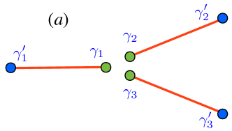
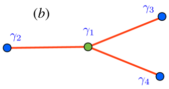
Figure 1: The usually discussed Y-junction setup. The initial configuration is shown in panel (a) and consists of three three Majorana states, $\gamma_{i}$, in the center and other three states, $\gamma_{i}^{\prime}$, at some distance. After hybridization, two out of three central Majorana states are split and the third one remains at zero energy. The resulting configuration is shown after renumbering in panel (b) and is described by the effective Hamiltonian (1).

We now parametrize this Hamiltonian by

$$u_{1}=u\cos\theta,\quad u_{2}=u\sin\theta\cos\phi,\quad u_{3}=u\sin\theta\sin\phi.$$ (2)

The parameter $u$ sets an overall scale, that is not important for our discussion, and a pair of angles $(\theta,\phi)$ represents a point on a unit sphere. The adiabatic evolution of ${\cal H}$ is viewed as a route, passed by this point on the sphere during the manipulation protocol.

The above Hamiltonian has two true (non-split) Majorana eigenstates, $\gamma_{\theta}$ and $\gamma_{\phi}$ (see below); we are following the notations of Ref. Karzig2015 It is convenient to combine these two states into one complex fermion $c=\gamma_{\theta}+i\gamma_{\phi}$. During an adiabatic evolution it acquires a Berry’s phase $c\to e^{i\alpha}c$, given by

$$2\alpha=-\oint\cos\theta\,{d\phi}=\int\sin\theta\,d\theta d\phi\,.$$ (3)

The simplest trajectory of adiabatic evolution corresponds to the case where one of the three parameters $u_{j}$ in Eq. (1) is zero. This relies on the exponentially small overlap between wave functions of Majorana fermions situated at spatially separated end points of the wires. Geometrically, it is depicted by three lines on the sphere, $\theta=\pi/2$, $\phi=\pi/2$ and $\phi=0$, shown in Fig. 2. To simplify the presentation, let us choose the initial conditions such that two computational Majoranas, $\gamma_{3,4}$, are decoupled from the ancilla Majoranas, $\gamma_{1,2}$, and from each other ($u_{1}\neq 0$ and $u_{2,3}=0$). This corresponds to the north pole in terms of the angular coordinates ($\theta=0$, for any value of $\phi$).

The evolution, that follows the trajectory $(0,0)\rightarrow(\pi/2,0)\rightarrow(\pi/2,\pi/2)\rightarrow(0,0)$ (represented in Fig. 2 by a red line ) encircles the solid angle $\pi/2$. As can be easily seen from the figure it encompasses one eighth of an entire sphere and is thus one eighth of its solid angle $4\pi$. After following this trajectory the wave function acquires the Berry’s phase $\pi/4$ that corresponds to the interchange of two “computational” Majoranas, $\gamma_{4}\to\pm\gamma_{3}$, $\gamma_{3}\to\mp\gamma_{4}$. Note, that this trajectory is special, because it satisfies the condition on the angles: either $\phi=0$ or $\theta=\pi/2$. This guarantees that Majorana states remain degenerate and the ground state is not affected by dephasing. If the trajectory deviates from this line and enters the area shown in green, the topological protection is lost, see below.

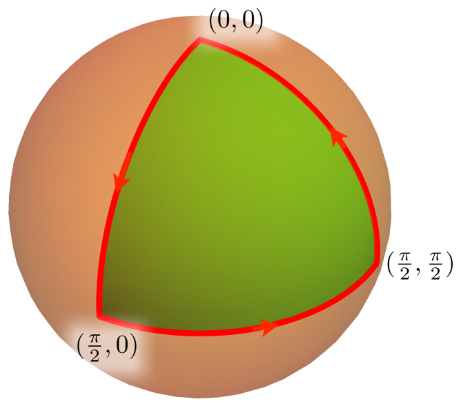
Figure 2: Unit sphere, representing the arbitrary Hamiltonian with four Majoranas. In simpler case of Y-junction the Hamiltonian (1) is parametrized by the angle on the sphere $(\theta,\phi)$, and the evolution along the red line leads to $\pi/4$ Berry’s phase. The case of X-junction, Eq. (6) is characterized by two points on the sphere, $(\theta,\phi)$, $(\bar{\theta},\bar{\phi})$, which parametrize the Hamiltonian with two non-split Majorana states. Possible trajectories leading to $\pi/8$ Berry’s phase are discussed in the main text, one of them given by the same red line now describing the variation in $\theta$, $\phi$ while $\bar{\phi}$ is fixed.

We note here in passing, that if no concern for the topological protection were involved, the whole family of simple trajectories would provide the desired value of he Berry’s phase. Explicitly we write in terms of (1),

$$u_{1} =1-\sin^{2}\phi\tan^{2}\theta_{0},\quad u_{2}=2\sin^{2}\phi\tan\theta_{0},$$ (4)

$$u_{3} =\sin 2\phi\tan\theta_{0}.$$

The value $u=\sqrt{u_{1}^{2}+u_{2}^{2}+u_{3}^{2}}=1+\sin^{2}\phi\tan^{2}\theta_{0}$ depends on $\phi$, but it is irrelevant here. It can be easily verified that upon the variation $\phi\in(0,\pi)$ the phase $2\alpha=2\pi(1-\cos\theta_{0})$, which shows that for $\cos\theta_{0}=7/8,5/8,3/8,1/8$ we should have $\alpha=\pi/8,3\pi/8,5\pi/8,7\pi/8$, respectively. Two examples of such circular trajectories are shown in Fig. 3. The apparent advantage of the parametrization (4) is the absence of sharp turning points during the adiabatic evolution (cf. Karzig2015 ) which is characterized only by the harmonics $e^{\pm 2i\phi}$.

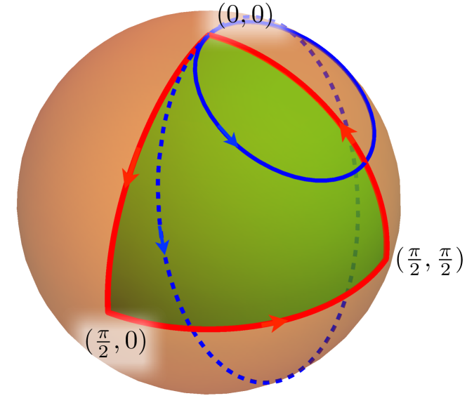
Figure 3: Two possible trajectories in case of Y-junction, leading to $\pi/8$ Berry’s phase, are discussed in text. The first one (solid blue line) is a circle centered at $\cos\theta_{0}=7/8$, leading to $\alpha=\pi/8$. Another circle is shown by dashed blue line, also passes via the north pole and is centered at $\cos\theta_{0}=3/8$, it produces $\alpha=5\pi/8$ .

It should be stressed that there is no way to realize $\pi/8$ state within this setup in a topologically protected manner, and one inevitably ends up in a situation in which all three tunneling amplitudes are finite ($u_{j}\neq 0$) Karzig2015 . The sizable hopping $u_{j}$ between $\gamma$’s appears if the distance between them is shorter that the characteristic correlation length. If Majorana fermions $\gamma_{2,3,4}$ are all close to $\gamma_{1}$ it implies that the distance between $\gamma_{2}$ and $\gamma_{3}$ is of the same order. Therefore one cannot neglect the coupling between $\gamma_{2}$ and $\gamma_{3}$, which is absent in Eq. (1). In this case we generally expect that the hopping amplitudes between all $\gamma$’s are non-zero. This impedes the quantum computation, because the degeneracy of the ground state has been removed, unless the coupling constants are tuned in a special way. Now on we focus on this case.

III X-junction

We consider a system of four connected wires with Majorana end modes, shown in Fig.4a, that host eight Majorana states. However the interaction between four Majorana fermions at the center is parametrically stronger than with the Majorana states at the ends and should be considered at the first stage, as described for Y-junction in Appendix C of Ref. Karzig2015 . If there are no special symmetries imposed on the system the degeneracy of the central states is completely lifted, and the remaining degrees of freedom are four weakly coupled Majorana states $\gamma_{j}^{\prime}$. Their Hamiltonian (after suppressing prime symbol) is given by

$${\cal H}=\tfrac{i}{2}\sum_{kl}H_{kl}\gamma_{k}\gamma_{l}$$ (5)

where

$$H =\begin{pmatrix}0,&u_{1}+\bar{u}_{1},&u_{2}+\bar{u}_{2},&u_{3}+\bar{u}_{3}\\ \cdot&0,&-u_{3}+\bar{u}_{3},&u_{2}-\bar{u}_{2}\\ \cdot&\cdot&0,&-u_{1}+\bar{u}_{1}\\ \cdot&\cdot&\cdot&0\end{pmatrix}$$ (6)

is a skew-symmetric matrix. The special case of pairwise equality ($u_{j}=\bar{u}_{j}$) corresponds to Eq. (1).

Of course one cannot rule out the accidental symmetry which may result in a setup where six Majorana states remain gapless. Though this situation is possible from a mathematical point of view, it is highly unlikely to occur, unless it is specially tuned. Therefore we assume that the nearby Majorana states at the center of the junction are gapped, while four at the far ends remain gapless. Such tuning can be accomplished by applying external gates and magnetic flux, as was discussed in details in Refs. Halperin2012 ; Romito2012 ; Hyart2013 . Clearly, the distance between Majorana states restricts a minimal size of the gates. It is therefore reasonable to assume that the larger distance between end Majoranas, $\gamma^{\prime}_{j}$ in Fig. 4a, allows some flexibility for changing the parameters in Eq.  (6).

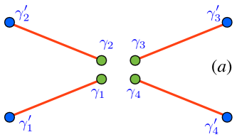
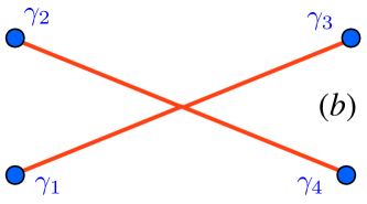
Figure 4: Two possible realizations of the X-junction setup described by the Hamiltonian (6). The panel (a) assumes four TI wires with endpoint Majorana states, four of them, $\gamma_{i}^{\prime}$, are far apart and four in the center, $\gamma_{i}$, are close enough to be described by the hopping Hamiltonian (6). If no special condition on this Hamiltonian is imposed, then four central Majorana states are fully split and disappear from the discussion, as shown in panel (b). The Hamiltonian (6) now refers to the remaining four Majorana states.

Because matrix $H$ is skew symmetric, it can be decomposed into a sum

$$H=\sum_{j=1}^{3}(u_{j}g_{j}+\bar{u}_{j}\bar{g}_{j}),$$ (7)

where $g_{1,2,3}$ ($\bar{g}_{1,2,3}$ ) are the generators of right (left) isoclinic subgroup of $SO(4)$ group, with the standard commutation relations $[g_{i},g_{j}]=2\epsilon_{ijk}g_{k}$ , $[\bar{g}_{i},\bar{g}_{j}]=-2\epsilon_{ijk}\bar{g}_{k}$. Importantly, the generators of left and right isoclinic subgroup commute, $[g_{i},\bar{g}_{j}]=0\,.$ The convenience of the above decomposition of $H$ becomes evident after performing a unitary transformation,

$$H\to UHU^{-1},$$ (8)

with $U$ belonging to $SO(4)$ group. It is known that any $U$ can be represented as a product $U=U_{L}U_{R}$ with

$$U_{R}=\exp\Big{(}\sum_{j=1}^{3}\alpha_{j}g_{j}\Big{)},\quad U_{L}=\exp\Big{(}\sum_{j=1}^{3}\bar{\alpha}_{j}\bar{g}_{j}\Big{)}.$$ (9)

Since $g_{j}$ and $\bar{g}_{j}$ commute, one finds

$$UHU^{-1}=\sum_{j=1}^{3}(u_{j}U_{R}g_{j}U_{R}^{-1}+\bar{u}_{j}U_{L}\bar{g}_{j}U_{L}^{-1}).$$ (10)

This decomposition implies that the triples $(u_{1},u_{2},u_{3})$ and $(\bar{u}_{1},\bar{u}_{2},\bar{u}_{3})$ are transformed within themselves according to $SO(3)$ group, that preserves the “lengths” of the vectors $u=\sqrt{u_{1}^{2}+u_{2}^{2}+u_{3}^{2}}$ and $\bar{u}=\sqrt{\bar{u}_{1}^{2}+\bar{u}_{2}^{2}+\bar{u}_{3}^{2}}$ invariant. One can easily show that the eigenvalues of ${\cal H}$ are $\pm(u+\bar{u})/2$ and $\pm(u-\bar{u})/2$. Because eigenvalues are preserved by unitary transformation, so are the values of $u$ and $\bar{u}$. Therefore, for the case where $u=\bar{u}$ two Majorana states (out of four) remain degenerate even though the components $u_{j}$, $\bar{u}_{j}$ are not equal.

Assuming that there are two non-split Majorana states without loss of generality we assume $u=\bar{u}=1$. The parametrization of the vectors $u$ and $\bar{u}$ by the angles (2), represents the Hamiltonian in new coordinates $(\theta,\phi,\bar{\theta},\bar{\phi})$ that correspond to two points on a unit sphere. For a pairwise equality $u_{k}=\bar{u}_{k}$, $k=1,2,3$ the two points merge to one, reproducing the familiar form of Y-junction Hamiltonian(1).

Now we employ this parametrization to calculate the Berry’s phase acquired by wave-function during the adiabatic evolution. Note, that the concept of adiabatic evolution in the present case needs a special justification, due to two-fold degeneracy of the zeroth-energy state. One may formally justifies the procedure by infinitesimal deformation $u=1+\epsilon$ , $\bar{u}=1-\epsilon$, and finally sending $\epsilon\to+0$. The adiabatic evolution of the state with the energy $\epsilon$, is determined by the linear combination $c^{\dagger}=\sum_{k=1}^{4}A_{k}\gamma_{k}$, where

$$\mathbf{A}= \tfrac{1}{2}\big{(}-\sin\theta_{+}\sin\phi_{-}-i\sin\theta_{-}\cos\phi_{-},$$ (11)

$$-\sin\theta_{+}\cos\phi_{-}+i\sin\theta_{-}\sin\phi_{-},$$

$$\cos\theta_{+}\cos\phi_{+}+i\cos\theta_{-}\sin\phi_{+},$$

$$\cos\theta_{+}\sin\phi_{+}-i\cos\theta_{-}\cos\phi_{+}\big{)}.$$

Here we used the notations $|\mathbf{A}|^{2}=\langle A|A\rangle=1/2$, and $\theta_{\pm}=(\theta\pm\bar{\theta})/2,\quad\phi_{\pm}=(\phi\pm\bar{\phi})/2$.

Clearly, the state with the energy $-\epsilon$ is given by $c=\sum_{k=1}^{4}A^{*}_{k}\gamma_{k}$. The geometrical phase, $\alpha$, acquired by the wave function during the evolution is given by

$$\frac{d\alpha}{dt}=\langle A|i\frac{d}{dt}|A\rangle=-\frac{1}{4}\left(\cos\theta\frac{d\phi}{dt}+\cos\bar{\theta}\frac{d\bar{\phi}}{dt}\right).$$ (12)

Let us now assume that evolution follows the closed trajectory and the final configuration is the same as the initial one, $(\theta,\phi,\bar{\theta},\bar{\phi})$. In this case, the Berry’s phase can be written as the integral over the closed path

$$2\alpha=-\frac{1}{2}\oint\left(\cos\theta\,{d\phi}+\cos\bar{\theta}\,{d\bar{\phi}}\right).$$ (13)

If initially $\mathbf{A}$ is a linear combination of $\gamma_{3,4}$, then the trajectory starts from the north pole ($\theta=\bar{\theta}=0$). Using Stokes’ theorem one transforms the line integral to the area integral

$$2\alpha=\frac{1}{2}\int\sin\theta\,d\theta d\phi+\frac{1}{2}\int\sin\bar{\theta}\,d\bar{\theta}d\bar{\phi}\,.$$ (14)

As we see, the geometric phase is a sum of two contribution. In the limit of $\theta=\bar{\theta}$, $\phi=\bar{\phi}$ one reproduces Eq. (3). In general case, however, there is a large freedom in choosing the trajectories, that are consistent with quantum computations. This allows us to generate almost Berry’s phase with any values. We will now demonstrate two simple examples.

At first we discuss a setup where the condition $\theta=\bar{\theta}$ is maintained during the entire cycle. Examining Eq.(14), we see that the corresponding Berry’s phase is essentially given by the previous formula (3) with the replacement $\phi\to\phi_{+}=(\phi+\bar{\phi})/2$. It means that in this type of evolution the difference $\phi_{-}$ between $\phi$ and $\bar{\phi}$ plays no role, and does not contribute to Berrys’ phase. This property might prove to be useful in error correction protocols such as, e.g., proposed in Karzig2015 .

In the second protocol we consider, the value of $\bar{\phi}$ is fixed, and the overall Berry’s phase is given only by the first integral in (14), which is one half of the expression (3). In particular, the desired value of $\alpha=\pi/8$ is provided by the previous trajectory around the octant of the sphere, Fig. 2, explicitly defined by $(\theta,\phi):(0,0)\to(\pi/2,0)\to(\pi/2,\pi/2)\to(0,\pi/2)$. The endpoints of the trajectory in second pair of coordinates $(\bar{\theta},\bar{\phi})$ should corresponds to the north pole, $\bar{\theta}=0$. The intermediate values of $\bar{\theta}$ are unimportant, and this additional degree of freedom may be helpful in discussing possible ways to reduce the errors in $\alpha$, see Ref.Karzig2015 .

The explicit form of the X-junction Hamiltonians, corresponding to two cases above, is shown in Appendix A.

IV Conclusions and outlook

In this paper we studied the manipulation of Majorana fermions coupled by X-junction. Unlike a more conventional Y-junction geometry, this setup requires a special tuning, in order to maintain the degeneracy of its ground state. The bright side of this method is a big parameter space that allows to perform necessary unitary transformations. Within this space there is a surface, where two Majorana bound states remain non-split. This surface is preserved under a group of unitary transformations, that factorizes into right and left isoclinic groups. Provided that the coupling of the junctions are changed in accordance with this symmetry the acquired phase is unaffected by the dephasing, and the junction can be used as a quantum gate. We proposed a few examples of adiabatic manipulations, that are consistent with this requirement, and calculate the corresponding Berry’s phase. In particular, the trajectories generating the vlaue $\alpha=\pi/8$, as well as other simple fractions of $\pi$, are demonstrated.

The natural extension of this analysis are junctions with five and more connectors. In this case, the system has a higher symmetry, and one expects more ways to perform the dephasing-free unitary transformations.

Aiming at applications, we understand that in possible realization the dephasing due to noise in the control gates could be quite substantial so that the X-junction would not be very different from any other non-topological qubit. The previously discussed Y-junction configuration is not immune to decoherence, which enters mainly via the $\pi/8$ gate. Thus it would be interesting to know if the X-junction, with generally absent topological protection, could compete in this respect with the Y-junction geometry. Particularly it is yet to be seen, whether one can design a physical realization, that locks the junction on to dephasing-free surfaces on the hardware level. Since the couplings in the Hamiltonian are influenced by external noise, it implies a design where noise affects a few couplings in a correlated manner. Unfortunately at this point, we were not able to propose a design based on realistic elements, where this locking takes place. However, even though a topologically protected quantum computation remains evasive, it may happen that dephasing time for a particular device will be sufficiently long for application. Our work lays a mathematical foundation for constructing quantum gates via X-junction.

Appendix A

In this appendix we present an explicit form for the effective Hamiltonian that correspond to the protocols suggested above. For the case $\theta=\bar{\theta}$ the Hamiltonian is given (up to the overall scale) by

$$H = \begin{pmatrix}0,&a,&b_{1},&b_{2}\\ \cdot&0,&b_{3},&b_{4}\\ \cdot&\cdot&0,&0\\ \cdot&\cdot&\cdot&0\end{pmatrix},$$ (15)

where we define

$$a =\cos\theta,$$

$$b_{1} =\sin\theta\cos\phi_{-}\cos\phi_{+},\quad b_{2}=\sin\theta\cos\phi_{-}\sin\phi_{+},$$

$$b_{3} =-\sin\theta\sin\phi_{-}\cos\phi_{+},\quad b_{4}=-\sin\theta\sin\phi_{-}\sin\phi_{+}.$$

This shows that the hopping amplitude between $\gamma_{3}$ and $\gamma_{4}$ is zero during the whole cycle.

In the second protocol discussed after Eq. (14) the value of $\bar{\phi}$ is fixed, and we set $\bar{\phi}=\pi/2$ for definiteness. We denote $c=\cos\bar{\theta}$, $s=\sin\bar{\theta}$ for brevity, then the Hamiltonian acquires the form

$$H=\begin{pmatrix}0&c+\cos\theta&\sin\theta\cos\phi&s+\sin\theta\sin\phi\\ \cdot&0&s-\sin\theta\sin\phi&\sin\theta\cos\phi\\ \cdot&\cdot&0&c-\cos\theta\\ \cdot&\cdot&\cdot&0\\ \end{pmatrix}.$$ (16)

Notice that (16) allows for non-vanishing coupling between $\gamma_{3}$ and $\gamma_{4}$ during manipulation. The endpoints of the trajectory should correspond to $c=1$, $s=0$, which is the north pole in coordinates $(\bar{\theta},\bar{\phi})$. The intermediate values of $c$, $s$ are unimportant for Berry’s phase.

References

- (1) M.A. Nielsen and I.L. Chuang, ”Quantum Computation and Quantum Information” (Cambridge Univ. Press, Cambridge, 2000).
- (2) A. Kitaev, Ann. Phys. 303, 2 (2003).
- (3) D. A. Ivanov Phys. Rev. Lett. 86, 268 (2001).
- (4) R. M. Lutchyn, J. D. Sau, and S. Das Sarma, Phys. Rev. Lett. 105, 077001 (2010).
- (5) Y. Oreg, G. Refael, and F. von Oppen, Phys. Rev. Lett. 105, 177002 (2010).
- (6) L. Fu and C. L. Kane, Phys. Rev. Lett. 100, 096407 (2008).
- (7) J. Linder, Y. Tanaka, T. Yokoyama, A. Sudbø, and N. Nagaosa, Phys. Rev. Lett. 104, 067001 (2010).
- (8) J. D. Sau, R. M. Lutchyn, S. Tewari, and S. Das Sarma, Phys. Rev. Lett. 104, 040502 (2010).
- (9) J. Alicea, Phys. Rev. B 81, 125318 (2010).
- (10) M. Sato and S. Fujimoto, Phys. Rev. B 79, 094504 (2009).
- (11) P. A. Lee, arXiv:0907.2681 (unpublished).
- (12) P. Ghosh, J. D. Sau, S. Tewari, and S. Das Sarma, Phys.Rev.B 82, 184525 (2010).
- (13) X.-L. Qi, T. L. Hughes, and S.-C. Zhang, Phys.Rev. B 82, 184516 (2010).
- (14) V. Mourik, K. Zuo, S.M. Frolov, S.R. Plissard, E.P.A. Bakkers, L.P. Kouwenhoven, Science 336, 1003 (2012).
- (15) D. Car, M.A. Verheijen, I. van Weperen, S.M. Frolov, L.P. Kouwenhoven, E.P.A.M. Bakkers, and S.R. Plissard, ”Formation and electronic properties of X- and T- shaped InSb nanowires and nanowire networks”, Proceeding of International Conference on Solid State Devices and Materials, Fukuoka, (2013).
- (16) M.T. Deng, C.L. Yu, G.Y. Huang, M Larsson, P Caroff, H.Q. Xu, Nano Letters 12 (12) (2012).
- (17) A. Das, Y. Ronen, Y. Most, Y. Oreg, M. Heiblum, H. Shtrikman, Nature Physics 8 887 (2012).
- (18) H.O.H. Churchill, V. Fatemi, K. Grove-Rasmussen, M.T. Deng, P. Caroff, H.Q. Xu, C.M. Marcus, Phys. Rev. B 87, 241401(R) (2013).
- (19) M.T. Deng, C.L. Yu, G.Y. Huang, M. Larsson, P. Caroff, H.Q. Xu Scientific Reports 4 7261, (2014).
- (20) A. Stern and N. H. Lindner, Science 339, 1179 1184 (2013).
- (21) J. Alicea, Y. Oreg, G. Refael, F. von Oppen, and M. P. A. Fisher, Nature Physics 7, 412 417 (2011).
- (22) J. D. Sau, D. J. Clarke, and S. Tewari, Phys. Rev. B 84, 094505 (2011).
- (23) B. I. Halperin, Y. Oreg, A. Stern, G. Refael, J. Alicea, and F. von Oppen, Phys. Rev. B 85, 144501 (2012).
- (24) A. Romito, J. Alicea, G. Refael, and F. von Oppen, Phys. Rev. B 85, 020502 (2012).
- (25) C. Beenakker, Annu. Rev. Condens. Matter Phys. 4, 113 (2013).
- (26) T. Hyart, B. van Heck, I. C. Fulga, M. Burrello, A. R. Akhmerov, and C. W. J. Beenakker, Phys. Rev. B 88, 035121 (2013).
- (27) T. Karzig, Y. Oreg, G. Refael, and M. H. Freedman, arXiv:1511.05161.