Exact “exact exchange” potential of two- and one-dimensional electron gases beyond the asymptotic limit

Abstract

The exchange-correlation potential experienced by an electron in the free space adjacent to a solid surface or to a low-dimensional system defines the fundamental image states and is generally important in surface- and nano-science. Here we determine the potential near the two- and one-dimensional electron gases (EG), doing this analytically at the level of the exact exchange of the density-functional theory (DFT). We find that, at $r_{\perp}\gg k_{F}^{-1}$, where $r_{\perp}$ is the distance from the EG and $k_{F}$ is the Fermi radius, the potential obeys the already known asymptotic $-e^{2}/r_{\perp}$, while at $r_{\perp}\lesssim k_{F}^{-1}$, but still in vacuum, qualitative and quantitative deviations of the exchange potential from the asymptotic law occur. The playground of the excitations to the low-lying image states falls into the latter regime, causing significant departure from the Rydberg series. In general, our analytical exchange potentials establish benchmarks for numerical approaches in the low-dimensional science, where DFT is by far the most common tool.

I Introduction

The image potential (IP) – a potential experienced by a test charge outside a semi-infinite medium, a slab, or a system of a lower dimensionality – is a fundamental concept of classical electrostatics Landau and Lifshitz (1960). It is widely believed, although never proven Lang and Kohn (1970); Dobson (1995); Constantin and Pitarke (2011), that the exchange-correlation (xc) part of the Kohn-Sham (KS) potential of the density-functional theory (DFT) Kohn and Sham (1965) must asymptotically reproduce the classical IP at large distances from an extended system. Much effort has been exerted over years to describe IP quantum-mechanically, both in order to account for the experimentally important image states at solid surfaces and at quasi-low-dimensional systems, and to gain better understanding of the non-trivial interrelations between DFT and classical physics Sham (1985); Harbola and Sahni (1987); Eguiluz et al. (1992); Horowitz et al. (2006, 2010); Constantin and Pitarke (2011); Qian (2012); Engel (2014a, b).

Regardless of the ultimate answer to the question of whether or not the xc potential (which is not a physical quantity) is equal in vacuum to the IP for a test charge (which is a physical quantity) , the determination of the former is fundamentally important in quantum physics. Indeed, it defines the KS band-structure of the system of interest, which step, followed by a calculation of the system’s response within the time-dependent DFT Zangwill and Soven (1980); Runge and Gross (1984); Gross and Kohn (1985, 1986), will produce excitations to image states (which are quite physical properties). While for semi-infinite media the problem still remains highly controversial Dobson (1995); Constantin and Pitarke (2011), for slabs it has been firmly established Horowitz et al. (2006); Engel (2014a) that, on the level of the optimized effective potential-exact exchange (OEP-EXX) Sharp and Horton (1953); Talman and Shadwick (1976); Görling and Levy (1994), the KS potential has the asymptotic $-e^{2}/r_{\perp}$, valid at large distances $r_{\perp}$ from the slab. However, apart from the thickness $a$, EG in the shape of a slab (quasi-2D EG) or a cylinder (quasi-1D EG), when considered quantum-mechanically, has a fundamental intrinsic parameter $k_{F}$ – the Fermi radius – and, therefore, even at $a=0$, two different regimes, at $r_{\perp}\gg k_{F}^{-1}$ and $r_{\perp}\lesssim k_{F}^{-1}$, can be anticipated.

At variance with a vast literature on the asymptotic behaviour of the xc potential, in this paper we are concerned with the potential in the whole space outside a 2(1)DEG. We solve this problem exactly and analytically at the EXX level of DFT and find that, at $r_{\perp}\lesssim k_{F}^{-1}$, but still in vacuum, the potential is qualitatively and quantitatively different from its asymptotic form $-e^{2}/r_{\perp}$. However, at larger distances $r_{\perp}\gg k_{F}^{-1}$, our potentials obey the correct asymptotic, which is known to be mandotary for slabs in general Engel (2014b). The non-asymptotic shape of the potential in the $r_{\perp}\lesssim k_{F}^{-1}$ region strongly affects experimentally important low-lying image states, causing significant deviations from the Rydberg series.

This paper is organized as follows: In Sec. II we derive a closed-form EXX potentials for quasi-2(1)DEG with one filled subband. In Sec. III we take the full confinement limit, obtaining analytical EXX potentials for 2D and 1D electron gases. In Sec. IV we visualize and discuss the results. In Sec. V we derive further insights from addressing the problem of quasi-2(1)DEG within the localized Hartree-Fock method. Section VI contains conclusions. In Appendix A we discuss the classical image potential in two and one dimensions. In Appendix B, finer details of the derivation of the main results are given. Atomic units ($e^{2}=\hbar=m_{e}=1$) are used throughout.

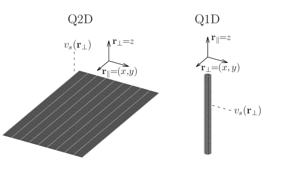
Figure 1: Schematics of quasi-2D (left) and quasi-1D (right) electron gases and the notations adopted.

II EXX potential of quasi-2(1)D electron gas with one subband filled

We start by considering a quasi $d$-dimensional ($d=2,1$), generally speaking, spin-polarized EG. The positively charged background with the $d$-dimensional density $n$ is strictly confined to the $xy$-plane and to the $z$-axis, for $d=2$ and $d=1$, respectively. We are concerned with the KS problem Kohn and Sham (1965) for spin-orbitals $\psi^{\sigma}_{i}(\mathbf{r})$ and eigenenergies $\epsilon^{\sigma}_{i}$, with the potential

$$v^{\sigma}_{s}(\mathbf{r})=v_{ext}(\mathbf{r})+v_{H}(\mathbf{r})+v^{\sigma}_{xc}(\mathbf{r}),$$ (1)

generally speaking, different for different spin orientations $\sigma$, where $v_{ext}(\mathbf{r})$, $v_{H}(\mathbf{r})=\int n(\mathbf{r}^{\prime})/|\mathbf{r}-\mathbf{r}^{\prime}|d\mathbf{r}^{\prime}$, and

$$v^{\sigma}_{xc}(\mathbf{r})=\frac{\delta E_{xc}}{\delta n^{\sigma}(\mathbf{r})}$$ (2)

are the external, Hartree, and xc potentials, respectively, $n^{\sigma}(\mathbf{r})$ are spin-densities, $n(\mathbf{r})=n^{\uparrow}(\mathbf{r})+n^{\downarrow}(\mathbf{r})$ is the particle-density, and $E_{xc}$ is the xc energy. For the latter we use the EXX part, which can be written as Slater (1951)

$$E_{x}=-\frac{1}{2}\int\frac{|\rho(\mathbf{r},\mathbf{r}^{\prime})|^{2}}{|\mathbf{r}-\mathbf{r}^{\prime}|}d\mathbf{r}d\mathbf{r}^{\prime},$$ (3)

where

$$\rho(\mathbf{r},\mathbf{r}^{\prime})=\sum\limits_{i\in occ}\phi_{i}(\mathbf{r})\phi_{i}^{*}(\mathbf{r}^{\prime})$$ (4)

is the density-matrix, the summation in Eq. (4) running over the occupied states only.

Let $\mathbf{r}_{\|}$ and $\mathbf{r}_{\perp}$ be the coordinate vectors parallel and perpendicular, respectively, to the extent of the EG. In other words, for $d=2$, $\mathbf{r}_{\|}$ is the radius-vector in the $xy$ plane and $\mathbf{r}_{\perp}$ is a vector in the $z$-direction, while for $d=1$ this is vice versa, as schematized in Fig. 1. Keeping in mind the subsequent zero-thickness limit, we assume one, at most, subband with the wave-function $\mu^{\sigma}_{0}(\mathbf{r}_{\perp})$ to be occupied for each spin direction. Therefore, all spin-orbitals with the same spin orientation have the same $\mathbf{r}_{\perp}$-dependence

$$\phi_{\mathbf{k}_{\|}}^{\sigma}(\mathbf{r})=\frac{e^{\mathrm{i}\mathbf{k}_{\|}\cdot\mathbf{r}_{\|}}}{\Omega^{1/2}}\mu^{\sigma}_{0}(\mathbf{r}_{\perp}),$$ (5)

where $\Omega$ is the normalization area or length, in the 2D and 1D cases, respectively. Then, by Eq. (4), for the density-matrix we can write

$$\rho(\mathbf{r},\mathbf{r}^{\prime})=\sum\limits_{\sigma}\mu^{\sigma}_{0}(\mathbf{r}_{\perp}){\mu^{\sigma}_{0}}^{*}(\mathbf{r}_{\perp}^{\prime})\rho^{\sigma}(\mathbf{r}_{\|}-\mathbf{r}^{\prime}_{\|}),$$ (6)

where

$$\rho^{\sigma}(\mathbf{r}_{\|})=\frac{1}{\Omega}\sum\limits_{|\mathbf{k}_{\|}|\leq k^{\sigma}_{F}}\!\!e^{\mathrm{i}\mathbf{k}_{\|}\cdot\mathbf{r}_{\|}},$$ (7)

$k^{\sigma}_{F}$ being the Fermi radii for the corresponding spin orientations. As will be seen below, the factorization (6) is the key property of 2(1)DEG with only one subband occupation, which makes possible the explicit solution to the EXX problem for these systems. Then, the exchange energy of Eq. (3) can be written as

$$\begin{split}E_{x}=-\frac{1}{2}\sum\limits_{\sigma}\int\frac{|\mu^{\sigma}_{0}(\mathbf{r}_{\perp})|^{2}|\mu^{\sigma}_{0}(\mathbf{r}_{\perp}^{\prime})|^{2}|\rho^{\sigma}(\mathbf{r}_{\|}-\mathbf{r}^{\prime}_{\|})|^{2}}{|\mathbf{r}-\mathbf{r}^{\prime}|}d\mathbf{r}d\mathbf{r}^{\prime}\\ =-\frac{1}{2}\sum\limits_{\sigma}\int\frac{n^{\sigma}(\mathbf{r})n^{\sigma}(\mathbf{r}^{\prime})|\rho^{\sigma}(\mathbf{r}_{\|}-\mathbf{r}^{\prime}_{\|})|^{2}}{(n^{\sigma})^{2}|\mathbf{r}-\mathbf{r}^{\prime}|}d\mathbf{r}d\mathbf{r}^{\prime},\end{split}$$ (8)

where the spin-density is

$$n^{\sigma}(\mathbf{r})=\rho^{\sigma}(\mathbf{r},\mathbf{r})=|\mu^{\sigma}_{0}(\mathbf{r}_{\perp})|^{2}n^{\sigma},$$ (9)

and $n^{\sigma}=\int n^{\sigma}(\mathbf{r})d\mathbf{r}_{\perp}$ is the $d$-dimensional uniform spin-density. By virtue of Eqs. (2), (8), and (9), the exchange potential evaluates explicitly to .

$$\begin{split}v^{\sigma}_{x}(\mathbf{r})&\!=\!\frac{\delta E_{x}}{\delta n^{\sigma}(\mathbf{r})}\!=\!-\frac{1}{(n^{\sigma})^{2}}\!\int\!\frac{n^{\sigma}(\mathbf{r}^{\prime})|\rho^{\sigma}(\mathbf{r}_{\|}\!-\!\mathbf{r}^{\prime}_{\|})|^{2}}{|\mathbf{r}-\mathbf{r}^{\prime}|}d\mathbf{r}^{\prime}\\ &=-\frac{1}{n^{\sigma}}\int\frac{|\mu^{\sigma}_{0}(\mathbf{r}^{\prime}_{\perp})|^{2}|\rho^{\sigma}(\mathbf{r}_{\|}-\mathbf{r}^{\prime}_{\|})|^{2}}{|\mathbf{r}-\mathbf{r}^{\prime}|}d\mathbf{r}^{\prime}.\end{split}$$ (10)

In Eq. (10) we easily recognize the Slater’s exchange potential Slater (1951). This leads us to the important conclusion that, for Q2(1)EG with only one subband filled for each spin component, EXX and the Slater’s potentials coincide exactly and, consequently, in this case, the EXX potential can be expressed in terms of the occupied states only. The latter becomes wrong when more subbands are filled .

Evaluation of integrals in Eq. (7) is straightforward, giving

$$\rho^{\sigma}(\mathbf{r}_{\|})=\frac{1}{2\pi r_{\|}}\left\{\begin{array}[]{ll}k_{F}^{\sigma}J_{1}(k_{F}^{\sigma}r_{\|}),&d=2,\\[5.0pt] 2\sin(k_{F}^{\sigma}r_{\|}),&d=1,\end{array}\right.$$ (11)

where $J_{1}(x)$ is the Bessel function of the first order. With the use of Eqs. (11), the integral over $\mathbf{r}^{\prime}_{\|}$ in Eq. (10) can be taken in special functions, resulting in

$$\begin{split}v^{\sigma}_{x}(r_{\perp})=-\int\frac{F_{d}(k_{F}^{\sigma}|\mathbf{r}_{\perp}-\mathbf{r}^{\prime}_{\perp}|)|\mu^{\sigma}_{0}(\mathbf{r}^{\prime}_{\perp})|^{2}}{|\mathbf{r}_{\perp}-\mathbf{r}^{\prime}_{\perp}|}d\mathbf{r}^{\prime}_{\perp},\end{split}$$ (12)

where

$$F_{2}(x)=1+\frac{L_{1}(2x)-I_{1}(2x)}{x},$$ (13)

$$F_{1}(x)=\frac{1}{2\pi}G_{2,4}^{2,2}\left[x^{2}\left|\begin{array}[]{l}\frac{1}{2},1\\[2.5pt] \frac{1}{2},\frac{1}{2},-\frac{1}{2},0\\ \end{array}\right.\right],$$ (14)

$L_{1}(x)$ and $I_{1}(x)$ are the first-order modified Struve and Bessel functions, respectively, and $G_{p,q}^{m,n}\left[x\left|\begin{array}[]{lll}a_{1},&...,&a_{p}\\ b_{1},&...,&b_{q}\\ \end{array}\right.\right]$ is the Meijer G-function Prudnikov et al. (1990); Wolfram Research (2015). Functions $F_{d}(x)$ are plotted in Fig. 2.

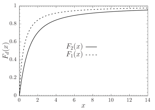
Figure 2: Functions $F_{2}(x)$ and $F_{1}(x)$ of Eqs. (13) and (14), which determine the 2D and 1D exchange potential, respectively.

III Full 2(1)D confinement limit

We now take the limit of the strictly $d$-dimensional (zero-thickness) electron gas. Then $|\mu^{\sigma}_{0}(\mathbf{r}_{\perp})|^{2}=\delta(\mathbf{r}_{\perp})$, and Eq. (12) reduces to

$$\begin{split}v^{\sigma}_{x}(r_{\perp})=-\frac{F_{d}(k_{F}^{\sigma}r_{\perp})}{r_{\perp}}.\end{split}$$ (15)

We emphasize that Eq. (15) was obtained for the mathematical idealization of an electron gas strictly confined to a plane (a straight line), as a limiting case of Eq. (12) for EG of a finite transverse extent.

The following zero-distance and asymptotic behaviour can be directly obtained from Eqs. (15) and (13) for the 2D case

$$v^{\sigma}_{x}(z=0)=-\frac{8k_{F}^{\sigma}}{3\pi},$$ (16)

$$v^{\sigma}_{x}(z\to\infty)\to-\frac{1}{z}+\frac{2}{\pi k_{F}^{\sigma}z^{2}}+...$$ (17)

and from Eqs. (15) and (14) for the 1D case

$$v^{\sigma}_{x}(\rho\to 0)\to\frac{k^{\sigma}_{F}}{\pi}[2\log(k^{\sigma}_{F}\rho)+2\gamma-3],$$ (18)

$$v^{\sigma}_{x}(\rho\to\infty)\to-\frac{1}{\rho}+\frac{1}{\pi k_{F}^{\sigma}\rho^{2}}+...,$$ (19)

where $\gamma\approx 0.5772$ is the Euler’s constant. At large distances, at the both dimensionalities, the potential respects the asymptotic $-1/r_{\perp}$.

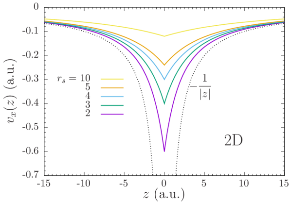
Figure 3: EXX potential of the spin-unpolarized 2DEG, obtained with Eqs. (15) and (13), versus the distance from the EG plane $z$, with the density parameter $r_{s}=(\pi n)^{-1/2}$ changing from 10 a.u. (top) to 2 a.u. (bottom). The dotted lines show the asymptotic $-1/|z|$.

IV Discussion

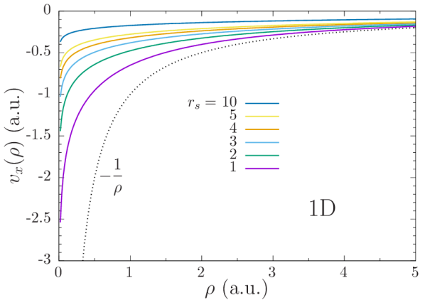
Figure 4: EXX potential of the spin-unpolarized 1DEG, obtained with Eqs. (15) and (14), versus the distance from the EG line $\rho$, with the density parameter $r_{s}=(2n)^{-1}$ changing from 10 (top) to 1 a.u. (bottom). The dotted line shows the asymptotic $-1/\rho$.

It is known that, in the general case, EXX-OEP potential cannot be expressed in terms of the occupied states only, but all, the occupied and empty, states are involved, and a complicated OEP integral equation must be solved to calculate this potential Sharp and Horton (1953); Talman and Shadwick (1976). It, therefore, may look surprising that a drastic simplification can be achieved in the case of 2(1)DEG with one subband filled, leading to Eq. (10), the latter expressed in terms of the occupied states only and not involving the OEP equation. To clarify this point, in Appendix B.1 we arrive at Eq. (10) following the traditional path of working out the EXX-OEP potential in terms of the eigenfunctions and the eigenenergies of all the states, seeing clearly how the simplifications arise due to the specifics of this system.

In Figs. 3 and 4, the EXX potentials of 2DEG and 1DEG, respectively, are plotted for a number of densities as functions of the distance from the EG. An important conclusion can be drawn from these figures together with the long-distance expansions (17) and (19): The more dense is the EG, the sooner the asymptotic is approached with the increase of the distance. The characteristic distance scale is the inverse Fermi radius $k_{F}^{-1}$, which separates two distinct regions, the asymptotic one realizing at $r_{\perp}\gtrsim k_{F}^{-1}$. We emphasize that in both regions there is no electron density, as is particularly clear with the strictly 2D and 1D (zero-thickness) EG.

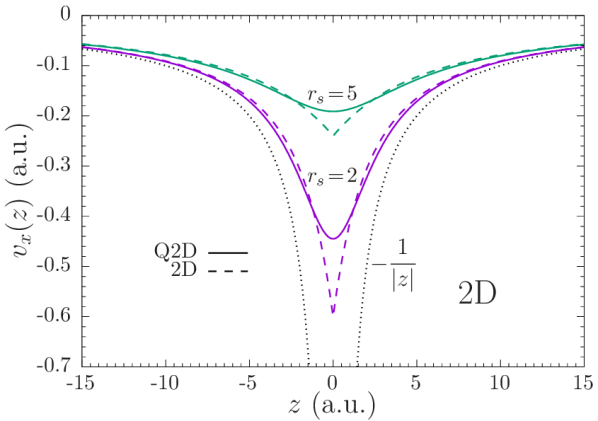
Figure 5: The EXX potential of spin-neutral Q2D EG with one subband filled (solid lines) compared to the analytical solution for the zero-thickness limit (dashed lines) for two values of the density parameter $r_{s}=2$ and $5$. The dotted lines show the asymptotic $-1/|z|$.

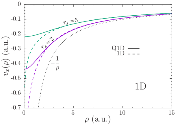
Figure 6: The same as Fig. 5 but for 1D case.

In Figs. 7 and 8 we present the exchange potential and the density for the spin-neutral and fully spin-polarized electron gas, in the 2D and 1D cases, respectively.

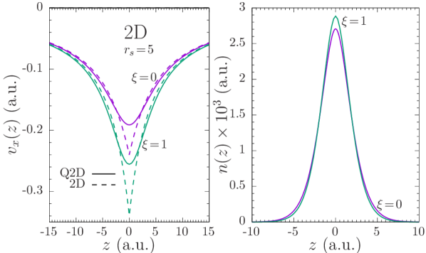
Figure 7: Left: Exchange potential as a function of the distance $z$ from the plane of the possitive background of quasi-2D (solid lines) and 2D (dashed lines) EG, for the spin-neutral ($\xi=0$) and fully spin-polarized ($\xi=1$) cases at the density-parameter $r_{s}=5$. Right: The corresponding particle densities of the Q2D EG.

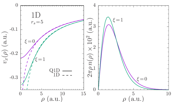
Figure 8: The same as Fig. 7, but for 1DEG.

A natural question arises: How relevant are the solutions obtained for strictly low-dimensional case to the realistic quasi-low-dimensional EG. To answer this, we return to Eq. (12) and solve the KS problem self-consistently using

$$\begin{split}&v_{ext,H}(\mathbf{r}_{\perp})=v_{ext}(\mathbf{r}_{\perp})+v_{H}(\mathbf{r}_{\perp})=2\pi\times\\ &\left\{\begin{array}[]{ll}\displaystyle\int\limits_{-\infty}^{\infty}\left(|z|-|z-z^{\prime}|\right)n(z^{\prime})dz^{\prime},&d=2,\\ \!\!\displaystyle\int\limits_{0}^{\infty}\!\!\rho^{\prime}n(\rho^{\prime})\log\dfrac{2\rho^{2}}{{\rho^{\prime}}^{2}\!+\!\rho^{2}\!+\!|{\rho^{\prime}}^{2}\!-\!\rho^{2}|}d\rho^{\prime},&d=1.\end{array}\right.\end{split}$$ (20)

Results for the EXX potential presented in Figs. 5 and 6, for the 2D and 1D cases, respectively, show that the zero-thickness limit of the EXX potential is a very good approximation to that of the quasi-low-dimensional EG except for very short distances from the system. At those distances, the electron-density is high (see Figs. 7 and 8), the deviation in this region being not surprising, since the potential is not that in vacuum any more. Results of the calculations for the spin-polarized EG are presented in Figs. 7 and 8.

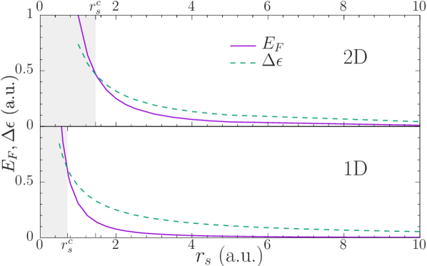
Figure 9: Diagrams of stability of Q2D (upper panel) and Q1D (lower panel) electron gases with one subband occupied. The Fermi energy $E_{F}=k_{F}^{2}/2$ and the distance $\Delta\epsilon$ between two lowest subbands are shown versus the density-parameter $r_{s}$. At $r_{s}<r_{s}^{c}$ (shaded areas, $r_{s}^{c}\approx 1.46$ and $0.72$, in 2D and 1D cases, respectively), more than one subbands are filled, invalidating the results of this theory. The diagrams refer to the spin-unpolarized case.

In Table 1 the low-lying eigenenergies of the 2D and Q2D EG are presented. The deviation of the EXX potential from $-1/r_{\perp}$ in the non-asymptotic region causes significant change in the spectra of the eigenenergies compared with the Rydberg series, $-\frac{1}{2n^{2}}$ and $-\frac{1}{2\left(n-\frac{1}{2}\right)^{2}}$, for 2D and 1D cases, respectively, where $n=1,2,...$ Hassoun (1981).

	Rydberg	$r_{s}=2$		$r_{s}=5$
$n$	series	2D	Q2D	2D	Q2D
1	0.500	0.360	0.511	0.164	0.204
2	0.125	0.161	0.196	0.092	0.103
3	0.056	0.102	0.117	0.064	0.070
4	0.031	0.066	0.073	0.045	0.048
5	0.020	0.048	0.052	0.035	0.037
6	0.014	0.036	0.038	0.027	0.028

Table 1: The first six eigenenergies (absolute values, a. u.) of the EXX KS hamiltonian of 2D and Q2D EG for two values of the density parameter $r_{s}=2$ and $5$, compared with the Rydberg’s series $1/(2n^{2})$.

Having found the analytical EXX potential of the strictly 2(1)DEG to be good approximations to the corresponding quasi-low-dimensional EG with one filled subband, we need to establish when the latter regime actually holds. This question is answered in the diagrams of the stability of the EG with one subband filled, presented in Fig. 9. For $r_{s}>r_{s}^{c}$ ($r_{s}^{c}\approx 1.46$ and $0.72$ in 2D and 1D cases, respectively) $E_{F}=k_{F}^{2}/2<\Delta\epsilon$, where $\Delta\epsilon$ is the subband gap, the state with one filled subband is stable. Otherwise, at $r_{s}<r_{s}^{c}$, it is energetically preferable to start filling the second subband. The latter regions, corresponding to high electron densities and to which our theory does not apply, are shaded at the diagrams.

For the sake of completeness, we write down the total energy in the one occupied subband regime. Using the DFT expression for energy

$$\begin{split}E&=\sum\limits_{i,\sigma}\epsilon^{\sigma}_{i}-\sum\limits_{\sigma}\int v^{\sigma}_{xc}(\mathbf{r})n^{\sigma}(\mathbf{r})d\mathbf{r}+E_{xc}\\ &-\frac{1}{2}\int v_{H}(\mathbf{r})n(\mathbf{r})d\mathbf{r}+\frac{1}{2}\int\frac{n^{+}(\mathbf{r})n^{+}(\mathbf{r}^{\prime})}{|\mathbf{r}-\mathbf{r}^{\prime}|}d\mathbf{r}d\mathbf{r}^{\prime},\end{split}$$ (21)

where the last term in Eq. (21) is the energy of the background positive charge $n^{+}(\mathbf{r})$, by virtue of Eqs. (8) and (10), we have for the energy per particle

$$\begin{split}\epsilon&=\epsilon_{K}+\epsilon_{sub}-\frac{1}{2n}\sum\limits_{\sigma}\int v^{\sigma}_{x}(\mathbf{r}_{\perp})n^{\sigma}(\mathbf{r}_{\perp})d\mathbf{r}_{\perp}\\ &-\frac{1}{2n}\int v_{ext,H}(\mathbf{r}_{\perp})\left[n(\mathbf{r}_{\perp})+n^{+}(\mathbf{r}_{\perp})\right]d\mathbf{r}_{\perp},\end{split}$$ (22)

where the kinetic and the subband energies are

$$\begin{split}&\epsilon_{K}=\frac{1}{2r_{s}^{2}}\left\{\begin{array}[]{ll}1+\xi^{2},&d=2,\\ \pi^{2}\left(1+3\xi^{2}\right)/48,&d=1,\end{array}\right.\end{split}$$ (23)

$$\epsilon_{sub}=\frac{1}{2}\left[\epsilon_{0}^{\uparrow}+\epsilon_{0}^{\downarrow}+\xi\left(\epsilon_{0}^{\uparrow}-\epsilon_{0}^{\downarrow}\right)\right],$$ (24)

and $\xi=(n^{\uparrow}-n^{\downarrow})/n$ is the spin polarization. In the zero-thickness limit $v_{ext,H}\!=\!0$, and the exchange energy per particle becomes $\epsilon_{x}=-\frac{2^{3/2}}{3\pi r_{s}}\left[\left(1+\xi\right)^{3/2}+\left(1-\xi\right)^{3/2}\right]$ and $\epsilon_{x}=-\infty$, for 2D and 1D cases, in accord with Refs. Tanatar and Ceperley, 1989 and Gold and Ghazali, 1990, respectively.

Our solutions, in particular, show that, while, in the general case, EXX requires the knowledge of all, occupied and empty, states, and solving of the optimized effective potential (OEP) integral equation is necessary, in the case of quasi-2(1)DEG with only one subband occupied, it is possible to avoid those complications, still remaining within the exact theory. In this context, we note that the localized Hartree-Fock potential (LHF) Della Sala and Görling (2001), which has proven a useful concept requiring the occupied states only and involving no OEP equation in the general case, yields results very close (often indistinguishable) to those of EXX and Hartree-Fock (HF) Della Sala and Görling (2001); Nazarov and Vignale (2015). Conceptually, LHF potential can be constructed independently from HF and EXX Nazarov (2013), within the scheme of the optimized propagation in time Nazarov (1985), and it is one of the realizations of the “direct energy” potentials Levy and Zahariev (2014, 2016). This is, therefore, very instructive to learn that, for 2(1)DEG with one filled subband, LHF coincides with both EXX and Slater’s potentials exactly up to a constant, as we show in the next section.

Here, it is instructive to draw the analogy with a singlet two-electron system with only one state filled, for which all the three potentials coincide Nazarov (2013); Nazarov and Vignale (2015). In the present case, although with an infinite number of electrons, the same property holds due to (i) the separation of the variables in the two perpendicular directions and (ii) to the system being uniform (the potential being flat) in the parallel direction.

V Equivalence of EXX and LHF for quasi-2(1)DEG with one filled subband

The purpose of this section is to prove that, within the one-filled-subband regime of 2(1)D electron gas, the localized Hartree-Fock (LHF) method and and exact exchange (EXX) are exactly equivalent.

We start by reminding the basic facts on the LHF potential Della Sala and Görling (2001) within the framework of the optimized-propagation method (OPM) Nazarov (1985, 2013); Nazarov and Vignale (2015). The LHF exchange potential $\tilde{v}^{\sigma}_{x}(\mathbf{r})$, experienced by electrons with the spin orientation $\sigma$, is a solution to the equation

$$\tilde{v}^{\sigma}_{x}(\mathbf{r})n^{\sigma}(\mathbf{r})=\int\left[\tilde{v}^{\sigma}_{x}(\mathbf{r}^{\prime})-\frac{1}{|\mathbf{r}-\mathbf{r}^{\prime}|}\right]|\rho^{\sigma}(\mathbf{r},\mathbf{r}^{\prime})|^{2}d\mathbf{r}^{\prime}+\int\frac{\rho^{\sigma}(\mathbf{r},\mathbf{r}^{\prime})\rho^{\sigma}(\mathbf{r}^{\prime},\mathbf{r}^{\prime\prime})\rho^{\sigma}(\mathbf{r}^{\prime\prime},\mathbf{r})}{|\mathbf{r}^{\prime}-\mathbf{r}^{\prime\prime}|}d\mathbf{r}^{\prime}d\mathbf{r}^{\prime\prime},$$ (25)

with the spin-resolved density-matrix defined as

$$\rho^{\sigma}(\mathbf{r},\mathbf{r}^{\prime})={\sum\limits_{i}}^{\sigma}\phi_{i}(\mathbf{r})\phi_{i}^{*}(\mathbf{r}^{\prime}),$$ (26)

where the superscript at the sum means that only the orbitals with the spin direction $\sigma$ are included. For integegral number of particles, Eq. (25) determines the potential up to the addition of an arbitrary constant $\tilde{v}^{\sigma}_{x}(\mathbf{r})\to\tilde{v}^{\sigma}_{x}(\mathbf{r})+c^{\sigma}$. Nazarov and Vignale (2015) A relation

$$\sum\limits_{\sigma}\left[\int\tilde{v}^{\sigma}_{x}(\mathbf{r})n^{\sigma}(\mathbf{r})d\mathbf{r}+\frac{1}{2}\int\frac{|\rho^{\sigma}(\mathbf{r},\mathbf{r}^{\prime})|^{2}}{|\mathbf{r}-\mathbf{r}^{\prime}|}d\mathbf{r}d\mathbf{r}^{\prime}\right]+\frac{1}{2}\int v_{H}(\mathbf{r})n(\mathbf{r})d\mathbf{r}=0$$ (27)

fixes this constant uniquely in the fully spin-polarized case, while in the presence of electrons of both spin orientations, it makes only one of the constants independent by fixing the quantity $c_{\uparrow}N_{\uparrow}+c_{\downarrow}N_{\downarrow}$, where $N_{\uparrow}$ and $N_{\downarrow}$ are the number of electrons with spin up and spin down, respectively. In both cases this fixes the total energy of the system, the electronic part of which is equal in OPM to the sum of the single-particle eigenenergies Nazarov and Vignale (2015).

For 2(1)DEG with only one subband filled

$$\rho^{\sigma}(\mathbf{r},\mathbf{r}^{\prime})=\mu^{\sigma}_{0}(\mathbf{r}_{\perp}){\mu^{\sigma}_{0}}^{*}(\mathbf{r}_{\perp}^{\prime})\rho^{\sigma}(\mathbf{r}_{\|}-\mathbf{r}^{\prime}_{\|}),$$ (28)

where $\rho^{\sigma}(\mathbf{r}_{\|})$ is given by Eq. (7). Substituting Eqs. (28) and (9) into Eq. (25) and canceling out $|\mu_{\sigma}(\mathbf{r}_{\perp})|^{2}$ from both sides, we can write

$$\begin{split}n^{\sigma}\tilde{v}^{\sigma}_{x}(\mathbf{r}_{\perp})=&-\int\frac{|\mu_{\sigma}(\mathbf{r}_{\perp}^{\prime})|^{2}|\rho^{\sigma}(\mathbf{r}_{\|}-\mathbf{r}^{\prime}_{\|})|^{2}}{|\mathbf{r}-\mathbf{r}^{\prime}|}d\mathbf{r}^{\prime}+\int\tilde{v}^{\sigma}_{x}(\mathbf{r}_{\perp}^{\prime})|\mu_{\sigma}(\mathbf{r}_{\perp}^{\prime})|^{2}|\rho^{\sigma}(\mathbf{r}_{\|}-\mathbf{r}^{\prime}_{\|})|^{2}d\mathbf{r}^{\prime}\\ &+\int\frac{|\mu_{\sigma}(\mathbf{r}_{\perp}^{\prime})|^{2}|\mu_{\sigma}(\mathbf{r}_{\perp}^{\prime\prime})|^{2}\rho^{\sigma}(\mathbf{r}_{\|}-\mathbf{r}_{\|}^{\prime})\rho^{\sigma}(\mathbf{r}^{\prime}_{\|}-\mathbf{r}_{\|}^{\prime\prime})\rho^{\sigma}(\mathbf{r}_{\|}^{\prime\prime}-\mathbf{r}_{\|})}{|\mathbf{r}^{\prime}-\mathbf{r}^{\prime\prime}|}d\mathbf{r}^{\prime}d\mathbf{r}^{\prime\prime},\end{split}$$ (29)

where we have explicitly written that the potential is a function of the perpendicular coordinate only. We notice, and this is crucial to our derivation, that the second and the third terms in the right-hand side of Eq. (29) are constants: The terms in question do not depend on $\mathbf{r}_{\perp}$, and the apparent dependence on $\mathbf{r}_{\|}$ is eliminated by the proper substitutions of the integration variables $\mathbf{r}_{\|}^{\prime}$ and $\mathbf{r}_{\|}^{\prime\prime}$. Recalling that Eqs. (25) are solvable up to arbitrary constants only, we can, therefore, write by virtue of Eq. (29)

$$\tilde{v}^{\sigma}_{x}(\mathbf{r}_{\perp})=v^{\sigma}_{x}(\mathbf{r}_{\perp})+c^{\sigma},$$ (30)

where $v^{\sigma}_{x}(\mathbf{r}_{\perp})$ is the EXX potential of Eq. (10). Substituting Eq. (30) into Eq. (27), we have

$$\sum\limits_{\sigma}c^{\sigma}N^{\sigma}=-\sum\limits_{\sigma}\left[\int v^{\sigma}_{x}(\mathbf{r})n^{\sigma}(\mathbf{r})d\mathbf{r}+\frac{1}{2}\int\frac{|\rho^{\sigma}(\mathbf{r},\mathbf{r}^{\prime})|^{2}}{|\mathbf{r}-\mathbf{r}^{\prime}|}d\mathbf{r}d\mathbf{r}^{\prime}\right]-\frac{1}{2}\int v_{H}(\mathbf{r})n(\mathbf{r})d\mathbf{r}.$$ (31)

As already mentioned above, within the framework of OPM, the electronic energy of a many-body system is a sum of the eigenvalues of its single-particle LHF hamiltonian (i.e., it is a “direct energy” potential Levy and Zahariev (2014, 2016)). Therefore, we can write

$$E=\sum\limits_{\sigma}{\sum\limits_{i}}^{\sigma}\tilde{\epsilon}_{i}+\frac{1}{2}\int\frac{n^{+}(\mathbf{r})n^{+}(\mathbf{r}^{\prime})}{|\mathbf{r}-\mathbf{r}^{\prime}|}d\mathbf{r}d\mathbf{r}^{\prime},$$ (32)

where the electrostatic energy of the positive background was added, as in the main text. Since, due to Eq. (30), the LHF Hamiltonian differs from the EXX one by the constants $c^{\sigma}$ only, we can write from Eq. (32)

$$E=\sum\limits_{\sigma}{\sum\limits_{i}}^{\sigma}\epsilon_{i}+\sum\limits_{\sigma}c^{\sigma}N^{\sigma}+\frac{1}{2}\int\frac{n^{+}(\mathbf{r})n^{+}(\mathbf{r}^{\prime})}{|\mathbf{r}-\mathbf{r}^{\prime}|}d\mathbf{r}d\mathbf{r}^{\prime},$$ (33)

where $\epsilon_{i}$ are the EXX eigenenergies. Finally, substituting Eq. (31) into Eq. (33) and comparing with Eq. (21), we conclude that the LHF and EXX total energies exactly coincide.

VI Conclusions

We have obtained explicit solutions to the problem of the exact exchange – optimized effective potential of quasi-two- and one-dimensional electron gases with one subband filled in terms of the density. It has been proven that the EXX potential, the localized Hartree-Fock potential, and the Slater’s potential all coincide with each other exactly (up to an arbitrary constant) for these systems.

By taking the limit of the zero-thickness [full 2(1)D confinement] of the respective electron gases, we have found exact analytical solutions to the static EXX problem for 2(1)DEG. We have identified a non-asymptotic regime, which realizes in the free space at distances less or comparable to the inverse Fermi radius of the electron gas. While our solutions reproduce the before known asymptotic of the exchange potential at large distances, at shorter distances the variance of the exchange potential from its asymptotic strongly affects the low-lying excited states, causing departure from the Rydberg series.

Within a wide range of the densities of the electron gases, our analytical potentials accurately approximate those of realistic quasi-2(1)D systems, as demonstrated by the comparison to the results of the self-consistent calculations beyond the zero-thickness limit. They, consequently, are expected to serve as efficient means to handle the general problem of the exchange potential and image states in the low-dimensional science.

As a by-product, our solutions extend a short list of analytical results known in the many-body physics.

Appendix A Classical image potential of 2(1)D conductor

Let 2(1)D conductor occupy a plane (line) $\mathbf{r}_{\perp}=\mathbf{0}$ and let a test charge $Q$ be positioned at $\mathbf{r}_{\perp}=\mathbf{R}_{\perp}$ and $\mathbf{r}_{\|}=\mathbf{0}$. The field of the test charge will cause a change in the electron-density distribution, which we denote $n_{1}(\mathbf{r}_{\perp})$. The latter is determined by the constancy of the potential at the plane (line) of the conductor

$$\frac{Q}{\sqrt{R_{\perp}^{2}+\mathbf{r}_{\|}^{2}}}-\int\frac{n_{1}(\mathbf{r}_{\|}^{\prime})}{|\mathbf{r}_{\|}^{\prime}-\mathbf{r}_{\|}|}d\mathbf{r}_{\|}^{\prime}=0,$$ (34)

by which we also fix the potential origin. Taking Fourier-transform with respect to $\mathbf{r}_{\|}$ we have

$$n_{1}(\mathbf{q}_{\|})=Q\frac{v_{\mathbf{q}_{\|}}(R_{\perp})}{v_{\mathbf{q}_{\|}}(0)},$$ (35)

where

$$v_{\mathbf{q}_{\|}}(\mathbf{r}_{\perp})=\int\frac{e^{-\mathrm{i}\mathbf{q}_{\|}\cdot\mathbf{r}_{\|}}}{\sqrt{\mathbf{r}_{\|}^{2}+\mathbf{r}_{\perp}^{2}}}d\mathbf{r}_{\|}.$$ (36)

In real space Eq. (35) yields for the density

$$n_{1}(\mathbf{r}_{\|})=\frac{Q}{(2\pi)^{d}}\int\frac{v_{\mathbf{q}_{\|}}(R_{\perp})}{v_{\mathbf{q}_{\|}}(0)}e^{\mathrm{i}\mathbf{q}_{\|}\cdot\mathbf{r}_{\|}}d\mathbf{q}_{\|}$$ (37)

and for its induced potential

$$\phi_{ind}(\mathbf{r}_{\|},\mathbf{r}_{\perp})=-\frac{Q}{(2\pi)^{d}}\int\frac{v_{\mathbf{q}_{\|}}(R_{\perp})v_{\mathbf{q}_{\|}}(r_{\perp})}{v_{\mathbf{q}_{\|}}(0)}e^{\mathrm{i}\mathbf{q}_{\|}\cdot\mathbf{r}_{\|}}d\mathbf{q}_{\|}.$$ (38)

The total energy of the system, which, being the work required to move the test charge from $\mathbf{R}_{\perp}$ to infinity and, therefore, is the image potential, is

$$E=Q\phi_{ind}(\mathbf{r}_{\|}=\mathbf{0},\mathbf{R}_{\perp})+\frac{1}{2}\int\frac{n_{1}(\mathbf{r}_{\|})n_{1}(\mathbf{r}^{\prime}_{\|})}{|\mathbf{r}_{\|}-\mathbf{r}^{\prime}_{\|}|}d\mathbf{r}_{\|}d\mathbf{r}^{\prime}_{\|},$$ (39)

which, by Eqs. (37) and (38) can be rewritten as

$$\begin{split}E&=-\frac{Q^{2}}{(2\pi)^{d}}\int\frac{v^{2}_{\mathbf{q}_{\|}}(R_{\perp})}{v_{\mathbf{q}_{\|}}(0)}d\mathbf{q}_{\|}+\frac{Q^{2}}{2(2\pi)^{d}}\\ &\times\int\frac{v^{2}_{\mathbf{q}_{\|}}(R_{\perp})}{v_{\mathbf{q}_{\|}}(0)}d\mathbf{q}_{\|}=-\frac{Q^{2}}{2(2\pi)^{d}}\int\frac{v^{2}_{\mathbf{q}_{\|}}(R_{\perp})}{v_{\mathbf{q}_{\|}}(0)}d\mathbf{q}_{\|}.\end{split}$$ (40)

2D-case

By Eq. (36), $v_{\mathbf{q}_{\|}}(R_{\perp})=\frac{2\pi}{q_{\|}}e^{-q_{\|}R_{\perp}}$, and Eq. (40) evaluates to

$$E=-\frac{Q^{2}}{4R_{\perp}},$$ (41)

which coincides with the result for a semi-infinite metal.

1D-case

By Eq. (36), $v_{\mathbf{q}_{\|}}(R_{\perp})=2K_{0}(q_{\|}R_{\perp})$, where $K_{n}(x)$ is the modified Bessel function of the second kind. Since $K_{0}(0)=\infty$, Eq. (40) evaluates to

$$E=0,$$ (42)

in accordance that the notion of the strictly 1D electron gas is inherently inconsistent and a finite width must be introduced for meaningful results Gold and Ghazali (1990). These complications are not, however, relevant to the purposes of the present work.

Appendix B Further particulars of the derivation of Eq. (10)

The derivation of Eq. (10) has been assuming that the system remains that with one subband filled [and, therefore, Eq. (8) holding] throughout the variational process. Here we show that this, indeed, is the case. Let us write the variation of the exchange energy

$$\delta E_{x}=\int v_{x}(\mathbf{r}_{\perp})\delta n(\mathbf{r})d\mathbf{r},$$ (43)

where, due to the symmetry of the problem, we have used the fact that $v_{x}$ is a function of the perpendicular coordinate only. Therefore, the variontions of the density which avarage out to zero in the parallel to the EG direction (which is necessary for the conservation of the number of particles) do not affect the the first order variation of $E_{x}$, the latter taken at the ground-state of the density. Therefore, with respect to finding the ground-state exchange potential for our systems, we need to consider the variations of the density which depend on $\mathbf{r}_{\perp}$ only.

By the chain rule, this leads to the variation of the KS potential $v_{s}$ as a function of $\mathbf{r}_{\perp}$ only, too. Since the variables $\mathbf{r}_{\perp}$ and $\mathbf{r}_{\|}$ separate in KS equations and since the ground-state occupied spin-orbitals (5) factorize with the same perpendicular part for all of them, it is obvious, that, upon a variation of $v_{s}^{\sigma}(\mathbf{r})$, the changed orbitals remain of the same form (5) with one and the same, changed, perpendicular part. In other words, through the variational procedure, the system remains that with only one subband filled.

B.1 Proof of Eq. (10) in terms of the orbital wave-functions and eigenenergies

Here we give an alternative proof of Eq. (10) which shows how the general EXX formalism leads to the Slater potential in the case of quasi 2(1)DEG with only one subband filled. We can write

$$\frac{\delta E_{x}}{\delta v_{s}^{\sigma}(\mathbf{r})}=\int\frac{\delta n(\mathbf{r}^{\prime})}{\delta v_{s}^{\sigma}(\mathbf{r})}\frac{\delta E_{x}}{\delta n^{\sigma}(\mathbf{r}^{\prime})}d\mathbf{r}^{\prime}=\int\chi_{s}^{\sigma}(\mathbf{r},\mathbf{r}^{\prime})v_{x}^{\sigma}(\mathbf{r}^{\prime})d\mathbf{r}^{\prime},$$ (44)

where we have used the chain rule, the definitions of $v_{x}^{\sigma}(\mathbf{r})$ and of the KS spin-density-response function $\chi^{\sigma}_{s}(\mathbf{r},\mathbf{r}^{\prime})$, and the symmetry of the latter in its two coordinate variables. The explicit expression of $\chi^{\sigma}_{s}(\mathbf{r},\mathbf{r}^{\prime})$ in terms of the KS wave-functions and eigenenergies is

$$\chi_{s}^{\sigma}(\mathbf{r},\mathbf{r}^{\prime})=\sum\limits_{\shortstack{\scriptsize{$i\in occ$} \\ \scriptsize{$j\not\in occ$}}}\frac{\psi^{\sigma*}_{i}(\mathbf{r})\psi_{j}^{\sigma}(\mathbf{r})\psi^{\sigma*}_{j}(\mathbf{r}^{\prime})\psi^{\sigma}_{i}(\mathbf{r}^{\prime})}{\epsilon_{i}-\epsilon_{j}}+c.c.$$ (45)

In the case of 2(1)D EG with the flat in-plane potential, the variables $\mathbf{r}_{\|}$ and $\mathbf{r}_{\perp}$ separate in the KS equations, $i$ ($j$) becomes a composite index $i=(\mathbf{k}_{\|i},n_{i})$, where $\mathbf{k}_{\|}$ is the parallel momentum, $n$ indexes the transverse bands, and

$$\epsilon^{\sigma}_{i}=\frac{k_{\|i}^{2}}{2}+\lambda_{n_{i}}^{\sigma},$$ (46)

$$\phi_{i}^{\sigma}(\mathbf{r})=\frac{e^{\mathrm{i}\mathbf{k}_{\|i}\cdot\mathbf{r}_{\|}}}{\Omega^{1/2}}\mu^{\sigma}_{n_{i}}(\mathbf{r}_{\perp}),$$ (47)

where $\mu^{\sigma}_{n_{i}}(\mathbf{r}_{\perp})$ are the wave-functions of the $(3-d)$-dimensional motion in the potential $v_{s}^{\sigma}(\mathbf{r}_{\perp})$, and $\lambda_{n_{i}}$ are the corresponding eigenenergies. We substitute Eqs. (45)-(47) into Eq. (44) and note that, by the symmetry of the problem, the left-hand side of Eq. (44) depends on $\mathbf{r}_{\perp}$ only and, therefore, we can average Eq. (44) in $\mathbf{r}_{\|}$ over $\Omega$ without changing it. Doing this and integrating over $\mathbf{r}^{\prime}_{\|}$ on the right-hand side with account of $v_{x}^{\sigma}(\mathbf{r}^{\prime})$ being a function of $\mathbf{r}^{\prime}_{\perp}$ only, we see that only $\mathbf{k}_{\|j}=\mathbf{k}_{\|i}$ contribute, leading to

$$\frac{\delta E_{x}}{\delta v_{s}^{\sigma}(\mathbf{r})}=n^{\sigma}\int\chi_{s}^{\sigma}(\mathbf{r}_{\perp},\mathbf{r}^{\prime}_{\perp})v_{x}^{\sigma}(\mathbf{r}^{\prime}_{\perp})d\mathbf{r}^{\prime}_{\perp},$$ (48)

where

$$\chi_{s}(\mathbf{r}_{\perp},\mathbf{r}^{\prime}_{\perp})=\sum\limits_{n=1}^{\infty}\frac{\mu^{\sigma*}_{0}(\mathbf{r}^{\prime}_{\perp})\mu^{\sigma}_{n}(\mathbf{r}^{\prime}_{\perp})\mu^{\sigma}_{0}(\mathbf{r}_{\perp})\mu^{\sigma*}_{n}(\mathbf{r}_{\perp})}{\lambda_{0}^{\sigma}-\lambda_{n}^{\sigma}}+c.c.,$$ (49)

and we have taken account of the fact that only one state with the wave-function $\mu_{0}^{\sigma}(\mathbf{r}_{\perp})$ is occupied in the transverse direction.

On the other hand, we can evaluate $\delta E_{x}/\delta v_{s}^{\sigma}(\mathbf{r})$ directly. By Eqs. (3) and (4)

$$E_{x}=-\frac{1}{2}\sum\limits_{\sigma}\sum\limits_{\shortstack{\scriptsize{$(i,\!\sigma)\!\in\!occ$} \\ \scriptsize{$(j,\!\sigma)\!\in\!occ$}}}\int\frac{\phi^{\sigma}_{i}(\mathbf{r})\phi_{j}^{\sigma*}(\mathbf{r})\phi_{j}^{\sigma}(\mathbf{r}^{\prime})\phi_{i}^{\sigma*}(\mathbf{r}^{\prime})}{|\mathbf{r}-\mathbf{r}^{\prime}|}d\mathbf{r}d\mathbf{r}^{\prime}.$$ (50)

Then, using the chain rule,

$$\begin{split}\frac{\delta E_{x}}{\delta v_{s}^{\sigma}(\mathbf{r})}\!=\!\!\!\!\!\sum\limits_{m\in occ}\int\!\left[\frac{\delta E_{x}}{\delta\phi_{m}^{\sigma}(\mathbf{r}^{\prime})}\frac{\delta\phi_{m}^{\sigma}(\mathbf{r}^{\prime})}{\delta v_{s}^{\sigma}(\mathbf{r})}\!+\!\frac{\delta E_{x}}{\delta\phi_{m}^{\sigma*}(\mathbf{r}^{\prime})}\frac{\delta\phi_{m}^{\sigma*}(\mathbf{r}^{\prime})}{\delta v_{s}^{\sigma}(\mathbf{r})}\right]\!d\mathbf{r}^{\prime}.\end{split}$$ (51)

Due to Eq. (50)

$$\frac{\delta E_{x}}{\delta\phi_{m}^{\sigma}(\mathbf{r}^{\prime})}\!=\!-\!\!\!\!\!\sum\limits_{(i,\sigma)\in occ}\!\int\!\frac{\phi^{\sigma}_{i}(\mathbf{r}^{\prime\prime})\phi_{m}^{\sigma*}(\mathbf{r}^{\prime\prime})\phi_{i}^{\sigma*}(\mathbf{r}^{\prime})}{|\mathbf{r}^{\prime}-\mathbf{r}^{\prime\prime}|}d\mathbf{r}^{\prime\prime},(m,\sigma)\!\in\!occ.$$ (52)

By the use of the perturbation theory, we can write

$$\frac{\delta\phi_{m}(\mathbf{r}^{\prime})}{\delta v_{s}^{\sigma}(\mathbf{r})}=\sum\limits_{l\neq m}\frac{\phi_{l}^{\sigma}(\mathbf{r}^{\prime})\phi_{m}^{\sigma}(\mathbf{r})\phi_{l}^{\sigma*}(\mathbf{r})}{\epsilon_{m}^{\sigma}-\epsilon_{l}^{\sigma}}.$$ (53)

Substitution of Eqs. (52) and (53) into Eq. (51) gives

$$\frac{\delta E_{x}}{\delta v_{s}^{\sigma}(\mathbf{r})}=-\sum\limits_{\shortstack{\scriptsize{$(m,\!\sigma)\!\in\!occ$} \\ \scriptsize{$(i,\sigma)\in\!occ$}}}\ \sum\limits_{l\neq m}\int\left[\frac{\phi^{\sigma}_{i}(\mathbf{r}^{\prime\prime})\phi_{m}^{\sigma*}(\mathbf{r}^{\prime\prime})\phi_{i}^{\sigma*}(\mathbf{r}^{\prime})\phi_{l}^{\sigma}(\mathbf{r}^{\prime})\phi_{m}^{\sigma}(\mathbf{r})\phi_{l}^{\sigma*}(\mathbf{r})}{|\mathbf{r}^{\prime}-\mathbf{r}^{\prime\prime}|(\epsilon_{m}^{\sigma}-\epsilon_{l}^{\sigma})}+c.c.\right]d\mathbf{r}^{\prime}d\mathbf{r}^{\prime\prime}.$$ (54)

Further, substituting Eqs. (46) and (47) into Eq. (54), we have

$$\begin{split}&\frac{\delta E_{x}}{\delta v_{s}^{\sigma}(\mathbf{r})}=-\frac{1}{\Omega^{3}}\sum\limits_{\shortstack{\scriptsize{$|\mathbf{k}_{\|i}|\leq k^{\sigma}_{F}$} \\ \scriptsize{$|\mathbf{k}_{\|m}|\leq k^{\sigma}_{F}$}}}\ \ \sum\limits_{(\mathbf{k}_{\|l},n_{l})\neq(\mathbf{k}_{\|m},0)}\\ &\int\left[\frac{e^{\mathrm{i}(\mathbf{k}_{\|i}-\mathbf{k}_{\|m})\cdot\mathbf{r}^{\prime\prime}_{\|}}\mu^{\sigma}_{0}(\mathbf{r}^{\prime\prime}_{\perp})\mu^{\sigma*}_{0}(\mathbf{r}^{\prime\prime}_{\perp})\mu^{\sigma*}_{0}(\mathbf{r}^{\prime}_{\perp})e^{\mathrm{i}(\mathbf{k}_{\|l}-\mathbf{k}_{\|i})\cdot\mathbf{r}^{\prime}_{\|}}\mu^{\sigma}_{n_{l}}(\mathbf{r}^{\prime}_{\perp})e^{\mathrm{i}(\mathbf{k}_{\|m}-\mathbf{k}_{\|l})\cdot\mathbf{r}_{\|}}\mu^{\sigma}_{0}(\mathbf{r}_{\perp})\mu^{\sigma*}_{n_{l}}(\mathbf{r}_{\perp})}{\left(\frac{k_{\|m}^{2}}{2}+\lambda_{0}^{\sigma}-\frac{k_{\|l}^{2}}{2}-\lambda_{n_{l}}^{\sigma}\right)|\mathbf{r}^{\prime}-\mathbf{r}^{\prime\prime}|}+c.c.\right]d\mathbf{r}^{\prime}d\mathbf{r}^{\prime\prime},\end{split}$$ (55)

where, again, it has been taken into account that the occupied orbitals have only one transverse band $\mu^{\sigma}_{0}(\mathbf{r}_{\perp})$.

Similar to the above, we average Eq. (55) over $\mathbf{r}_{\|}$ without changing it. This leads to only the terms with $\mathbf{k}_{\|l}=\mathbf{k}_{\|m}$ remaining, and gives

$$\frac{\delta E_{x}}{\delta v_{s}^{\sigma}(\mathbf{r})}=-\frac{1}{\Omega^{3}}\sum\limits_{\shortstack{\scriptsize{$|\mathbf{k}_{\|i}|\leq k^{\sigma}_{F}$} \\ \scriptsize{$|\mathbf{k}_{\|m}|\leq k^{\sigma}_{F}$}}}\ \sum\limits_{n=1}^{\infty}\int\left[\frac{|\mu^{\sigma}_{0}(\mathbf{r}^{\prime\prime}_{\perp})|^{2}\mu^{\sigma*}_{0}(\mathbf{r}^{\prime}_{\perp})\mu^{\sigma}_{n}(\mathbf{r}^{\prime}_{\perp})\mu^{\sigma}_{0}(\mathbf{r}_{\perp})\mu^{\sigma*}_{n}(\mathbf{r}_{\perp})e^{\mathrm{i}(\mathbf{k}_{\|m}-\mathbf{k}_{\|i})\cdot(\mathbf{r}^{\prime}_{\|}-\mathbf{r}^{\prime\prime}_{\|})}}{\left(\lambda_{0}^{\sigma}-\lambda_{n}^{\sigma}\right)|\mathbf{r}^{\prime}-\mathbf{r}^{\prime\prime}|}+c.c.\right]d\mathbf{r}^{\prime}d\mathbf{r}^{\prime\prime},$$ (56)

or, according to the definition (7),

$$\frac{\delta E_{x}}{\delta v_{s}^{\sigma}(\mathbf{r})}=-\frac{1}{\Omega}\sum\limits_{n=1}^{\infty}\int\left[\frac{|\mu^{\sigma}_{0}(\mathbf{r}^{\prime\prime}_{\perp})|^{2}\mu^{\sigma*}_{0}(\mathbf{r}^{\prime}_{\perp})\mu^{\sigma}_{n}(\mathbf{r}^{\prime}_{\perp})\mu^{\sigma}_{0}(\mathbf{r}_{\perp})\mu^{\sigma*}_{n}(\mathbf{r}_{\perp})|\rho^{\sigma}(\mathbf{r}^{\prime}_{\|}-\mathbf{r}^{\prime\prime}_{\|})|^{2}}{\left(\lambda_{0}^{\sigma}-\lambda_{n}^{\sigma}\right)|\mathbf{r}^{\prime}-\mathbf{r}^{\prime\prime}|}+c.c.\right]d\mathbf{r}^{\prime}d\mathbf{r}^{\prime\prime},$$ (57)

or, by Eq. (49) and integrating over $\mathbf{r}^{\prime}_{\|}$,

$$\frac{\delta E_{x}}{\delta v_{s}^{\sigma}(\mathbf{r})}=\!-\!\int\!d\mathbf{r}^{\prime}_{\perp}\chi_{s}^{\sigma}(\mathbf{r}_{\perp},\mathbf{r}^{\prime}_{\perp})\!\!\int\frac{|\mu^{\sigma}_{0}(\mathbf{r}^{\prime\prime}_{\perp})|^{2}|\rho^{\sigma}(\mathbf{r}^{\prime}_{\|}\!-\!\mathbf{r}^{\prime\prime}_{\|})|^{2}}{|\mathbf{r}^{\prime}-\mathbf{r}^{\prime\prime}|}d\mathbf{r}^{\prime\prime}.$$ (58)

Combining Eqs. (48) and (58), we have

$$\int d\mathbf{r}^{\prime}_{\perp}\chi_{s}^{\sigma}(\mathbf{r}_{\perp},\mathbf{r}^{\prime}_{\perp})\left[n^{\sigma}v_{x}^{\sigma}(\mathbf{r}^{\prime}_{\perp})+\int\frac{|\mu^{\sigma}_{0}(\mathbf{r}^{\prime\prime}_{\perp})|^{2}|\rho^{\sigma}(\mathbf{r}^{\prime}_{\|}-\mathbf{r}^{\prime\prime}_{\|})|^{2}}{|\mathbf{r}^{\prime}-\mathbf{r}^{\prime\prime}|}d\mathbf{r}^{\prime\prime}\right]=0.$$ (59)

For Eq. (59) to hold, the expression in the square brackets must be a constant, which retrieves the exchange potential of Eq. (10) up to an arbitrary constant.

References

- Landau and Lifshitz (1960) L. D. Landau and E. M. Lifshitz, Electrodynamics of continuous media (Pergamon Press, New York and London, 1960).
- Lang and Kohn (1970) N. D. Lang and W. Kohn, “Theory of metal surfaces: Charge density and surface energy,” Phys. Rev. B 1, 4555–4568 (1970).
- Dobson (1995) J. F. Dobson, in Density Functional Theory, edited by E. K. U. Gross and R. M. Dreizler (Plenum, New-York, 1995) p. 393.
- Constantin and Pitarke (2011) L. A. Constantin and J. M. Pitarke, “Adiabatic-connection-fluctuation-dissipation approach to long-range behavior of exchange-correlation energy at metal surfaces: A numerical study for jellium slabs,” Phys. Rev. B 83, 075116 (2011).
- Kohn and Sham (1965) W. Kohn and L. J. Sham, “Self-consistent equations including exchange and correlation effects,” Phys. Rev. 140, A1133–A1138 (1965).
- Sham (1985) L. J. Sham, “Exchange and correlation in density-functional theory,” Phys. Rev. B 32, 3876–3882 (1985).
- Harbola and Sahni (1987) M. K. Harbola and V. Sahni, “Asymptotic structure of the Slater-exchange potential at metallic surfaces,” Phys. Rev. B 36, 5024–5026 (1987).
- Eguiluz et al. (1992) A. G. Eguiluz, M. Heinrichsmeier, A. Fleszar, and W. Hanke, “First-principles evaluation of the surface barrier for a Kohn-Sham electron at a metal surface,” Phys. Rev. Lett. 68, 1359–1362 (1992).
- Horowitz et al. (2006) C. M. Horowitz, C. R. Proetto, and S. Rigamonti, “Kohn-Sham exchange potential for a metallic surface,” Phys. Rev. Lett. 97, 026802 (2006).
- Horowitz et al. (2010) C. M. Horowitz, C. R. Proetto, and J. M. Pitarke, “Localized versus extended systems in density functional theory: Some lessons from the Kohn-Sham exact exchange potential,” Phys. Rev. B 81, 121106 (2010).
- Qian (2012) Z. Qian, “Asymptotic behavior of the Kohn-Sham exchange potential at a metal surface,” Phys. Rev. B 85, 115124 (2012).
- Engel (2014a) E. Engel, “Exact exchange plane-wave-pseudopotential calculations for slabs,” The Journal of Chemical Physics 140, 18A505 (2014a).
- Engel (2014b) E. Engel, “Asymptotic behavior of exact exchange potential of slabs,” Phys. Rev. B 89, 245105 (2014b).
- Note (1) See Appendix A for the classical image potential of 2(1)DEG.
- Zangwill and Soven (1980) A. Zangwill and P. Soven, “Density-functional approach to local-field effects in finite systems: Photoabsorption in the rare gases,” Phys. Rev. A 21, 1561–1572 (1980).
- Runge and Gross (1984) E. Runge and E. K. U. Gross, “Density-functional theory for time-dependent systems,” Phys. Rev. Lett. 52, 997 (1984).
- Gross and Kohn (1985) E. K. U. Gross and W. Kohn, “Local density-functional theory of frequency-dependent linear response,” Phys. Rev. Lett. 55, 2850–2852 (1985).
- Gross and Kohn (1986) E. K. U. Gross and W. Kohn, “Local density-functional theory of frequency-dependent linear response,” Phys. Rev. Lett. 57, 923–923 (1986).
- Sharp and Horton (1953) R. T. Sharp and G. K. Horton, “A variational approach to the unipotential many-electron problem,” Phys. Rev. 90, 317–317 (1953).
- Talman and Shadwick (1976) J. D. Talman and W. F. Shadwick, “Optimized effective atomic central potential,” Phys. Rev. A 14, 36–40 (1976).
- Görling and Levy (1994) A. Görling and M. Levy, “Exact Kohn-Sham scheme based on perturbation theory,” Phys. Rev. A 50, 196–204 (1994).
- Slater (1951) J. C. Slater, “A simplification of the Hartree-Fock Method,” Phys. Rev. 81, 385–390 (1951).
- Note (2) In Eq. (10), the 3D spin-density is varied at a fixed value of the -dimensional spin-density (and, therefore, ), which amounts to the conservation of the total number of particles. In Appendix B further particulars of the derivation are given. For an alternative proof of Eq. (10) in terms of the KS eigenfunctions and eigenenergies, see Appendix B.1.
- Note (3) In particular, this does not hold for a metal surface, where the Slater and OEP potentials differ Harbola and Sahni (1987).
- Prudnikov et al. (1990) A. P. Prudnikov, O. I. Marichev, and Yu. A. Brychkov, Integrals and Series, Vol. 3: More Special Functions (Gordon and Breach, Newark, NJ, 1990).
- Wolfram Research (2015) Wolfram Research, Mathematica, version 10.3 ed. (Champaign, Illinios, 2015).
- Note (4) Although, separately the external and Hartree potentials are infinite, their sum of Eq. (20) is finite.
- Hassoun (1981) G. Q. Hassoun, “One- and two-dimensional hydrogen atoms,” American Journal of Physics 49, 143–146 (1981).
- Tanatar and Ceperley (1989) B. Tanatar and D. M. Ceperley, “Ground state of the two-dimensional electron gas,” Phys. Rev. B 39, 5005–5016 (1989).
- Gold and Ghazali (1990) A. Gold and A. Ghazali, “Exchange effects in a quasi-one-dimensional electron gas,” Phys. Rev. B 41, 8318–8322 (1990).
- Della Sala and Görling (2001) F. Della Sala and A. Görling, “Efficient localized Hartree-Fock methods as effective exact-exchange Kohn-Sham methods for molecules,” The Journal of Chemical Physics 115, 5718–5732 (2001).
- Nazarov and Vignale (2015) V. U. Nazarov and G. Vignale, “Derivative discontinuity with localized Hartree-Fock potential,” The Journal of Chemical Physics 143, 064111 (2015).
- Nazarov (2013) V. U. Nazarov, “Time-dependent effective potential and exchange kernel of homogeneous electron gas,” Phys. Rev. B 87, 165125 (2013).
- Nazarov (1985) V. U. Nazarov, “Time-dependent variational principle and self-consistent field equations,” Mathematical Proceedings of the Cambridge Philosophical Society 98, 373–379 (1985).
- Levy and Zahariev (2014) M. Levy and F. Zahariev, “Ground-state energy as a simple sum of orbital energies in Kohn-Sham theory: A shift in perspective through a shift in potential,” Phys. Rev. Lett. 113, 113002 (2014).
- Levy and Zahariev (2016) M. Levy and F. Zahariev, “On augmented Kohn–Sham potential for energy as a simple sum of orbital energies,” Molecular Physics 114, 1162–1164 (2016).