Bidding policies for market-based HPC workflow scheduling

Abstract

This paper considers the scheduling of jobs on distributed, heterogeneous High Performance Computing (HPC) clusters. Market-based approaches are known to be efficient for allocating limited resources to those that are most prepared to pay. This context is applicable to an HPC or cloud computing scenario where the platform is overloaded.

In this paper, jobs are composed of dependent tasks. Each job has a non-increasing time-value curve associated with it. Jobs are submitted to and scheduled by a market-clearing centralised auctioneer. This paper compares the performance of several policies for generating task bids. The aim investigated here is to maximise the value for the platform provider while minimising the number of jobs that do not complete (or starve).

It is found that the Projected Value Remaining bidding policy gives the highest level of value under a typical overload situation, and gives the lowest number of starved tasks across the space of utilisation examined. It does this by attempting to capture the urgency of tasks in the queue. At high levels of overload, some alternative algorithms produce slightly higher value, but at the cost of a hugely higher number of starved workflows.

I Introduction

In recent years, computational performance has increasingly been achieved through increasing parallelism rather than increased single-core performance. This is mainly due to the exponential increase in power consumption required to run processors at higher clock speeds [9]. Processors have become multicore, and multicore processors have been grouped into clusters and networks of clusters, known as grids [12]. These High Performance Computing (HPC) systems have grown to be huge in scale, especially those that support the operations of cloud computing corporations.

Many kinds of work run on HPC systems are not independent. Instead, workflows (or jobs) are run that are made up of several individual pieces of software (tasks), each of which takes some input and produces some output. This leads to the notion of dependencies between tasks, which restrict tasks to starting only once all their dependencies have completed and their input data transmitted.

Large-scale systems such as these can experience periods of high demand. This can even extend into periods of overload, where work is arriving faster than it can be executed. HPC providers need to be able to effectively prioritise work during these periods to ensure the most important work is run. Cloud providers who sell computing capacity on the open market will wish to maximise their profits by running the work that is most valuable [23]. There are real costs to HPC providers for running work, so it may sometimes be more worthwhile to discard work whose value is too low than to run it.

Work is run on computing clusters because it is valuable to the users and organisations who submit it. This value can be represented as a real amount of money that users are willing to pay for their results. This value is not always fixed. This is because work returned earlier may allow users or organisations to be more productive, whereas some work may have no value at all if it is returned too late [5].

Scheduling large-scale computing systems has traditionally been done through list scheduling [8, 16]. This is where all the work in a queue is ranked by an appropriate metric, and allocated to hardware in sorted order. Where value is assigned to work, market-based principles can be applied to scheduling.

The usefulness of work on list scheduling can be employed in a market-based way. The values calculated for ranking in a list scheduler can instead be used as bids that each piece of work submits to an auctioneer. Past research has investigated using value as bids [10]. However, the bids can be different than just the values of jobs at a given moment in time. It has been shown [5] that in the context of list scheduling, ordering tasks by total job value does not necessarily give the highest overall value under overload.

This paper explores the effectiveness of different bidding policies in a market-based scheduling scenario. This is to evaluate which provide the highest value, especially in periods of overload when not all work is able to run.

II Literature Survey

Scheduling using market-based techniques has been studied over a long period, with pioneering early work by Sutherland in the 1960s [21]. Since then, a great deal of work has been done on the structure of markets, investigating which structures best promote economic efficiency. Auction-based markets have been looked at by Waldspurger et al. [24] whereas market-clearing techniques where resources are allocated to work until one or other is consumed were investigated by Miller and Drexler [17]. Lai et al. have examined doing the allocation of resources in proportion to the value of bids [13]. Popovici and Wilkes [18] investigated market-inspired admission control. Dube [7] gives a good survey of the state of this research and concludes that various different market structures all hold promise, showing the benefits of better allocation and greater decentralisaion (and hence scalability and fault-tolerance) than traditional schedulers.

A necessary part of a market based system is that jobs have a certain value to users, and that this value is represented in the market by their bids [10]. There has been much past work on scheduling to maximise the value of a workload [14]. The problem of maximising workload value where job value is a function of time was extensively researched by Locke [15] for systems schedulable by the Earliest Deadline First list scheduling policy, and has subsequently been applied to more general scheduling problems [5, 6].

It seems that there has been little research into using value curves rather than fixed job values when scheduling in a market-based context. This is likely because markets need a single price for each bid submitted by a job, not a curve. Yet in previous work [5], it has been shown that value curves can be used to create single ranking values for list scheduling at given times in a simulation. This paper will extend this approach by using these values as bids in a market-based framework.

III Models

To evaluate which bidding policies are best, the simulator previously developed by the authors [5] was extended to use a market-based scheduling system. This simulator implements several models representing the applications, the platform, the scheduling scheme and the means of representing and calculating value. The simulation takes place in a discrete-time environment, where all events happen on time ticks $\tau\in\mathbb{N^{\mathrm{0}}}$.

III-A Application Model

The application model represents the work to be run on the cluster. Tasks are non-pre-emptive, running to completion once they have begun. This represents the behaviour of the LSF/GridEngine systems commonly used to manage large HPC systems. This lack of pre-emption is less of a problem at scale than it might seem, because in large-scale systems, the turnover of work is sufficiently high. This means that it is very unlikely that any job will ever have to wait too long for something to finish so that it can start [4].

For the purposes of this paper, a single, non-preemptible piece of work will be known as a task, denoted $T^{i}$. Each task will run for a duration $T_{\mathtt{exec}}^{i}\in\mathbb{N^{\star}}$ on a number of cores $T_{\mathtt{cores}}^{i}\in\mathbb{N^{\star}}$ concurrently. A set of tasks is known as a job, denoted $J^{k}$. Tasks can only depend on other tasks within the same job and the successors of each task will be known as $T_{\mathtt{succ}}^{i}$ . The structure of the dependencies will be that of a Directed Acyclic Graph (DAG), which defines a topological ordering over the tasks in a job: a partial order that they must be run in.

Having a dependency graph means several other useful metrics about a job can be calculated. The upward rank [22] of tasks, $T_{\mathtt{R}}^{i}$, is defined as the longest route from any task to its latest-finishing successor: $\forall\,T^{j}\in T_{\mathtt{succ}}^{i}:T_{\mathtt{R}}^{i}=T_{\mathtt{exec}}^{i}+\max(T_{\mathtt{R}}^{j})$. Sorting tasks by their upward rank will give an ordering that respects the partial order of the dependencies. The upward rank is also useful to estimate the finish time of a job if a task is run immediately. As jobs only realise their value once they have finished, this estimate is useful for scheduling comparisons at runtime.

The critical path [11] of a job, $J_{\mathtt{CP}}^{k}$, is equivalent to the largest upward rank of any of its component tasks: $\forall\,T^{i}\in J_{\mathtt{}}^{k}:J_{\mathtt{CP}}^{k}=\max\left(T_{R}^{i}\right)$ [22]. This is the length of time that the job would take to execute if the number of cores requied was unbounded, which is equivalent to its minimum execution time.

III-B Platform Model

The basic unit of the platform model is an execution core. Each cluster is made up of a number of cores. Multicore tasks must execute within a single cluster, and consume a number of cores for the duration of their execution. Cores are not shared between executing tasks. Within a cluster, cores are assumed to have negligible communication delays between them. For example, this could be due to all cores sharing a single networked file system. In the HPC context considered, execution times are measured in hours to days, so the highest-speed communications within cores on the same multicore processor or within the same server can reasonably be assumed to be negligible.

Clusters communicate through a central router. Delays are present for data transfers between clusters, and are adjustable using the Communication to Computation Ratio (CCR), supplied as an input to the simulations. For a task executing for $T_{\mathtt{exec}}^{i}$, the time taken for data transfer would be $T_{\mathtt{exec}}^{i}\times CCR$.

Heterogoneity is present in the model to a limited degree. Tasks and cluster cores have Kinds, which must match for a task to be able to run on a cluster. A task will always run for the same amount of time on clusters of the same kind. Each cluster is made up of cores of only one kind. This means that for jobs where tasks require different kinds, some network communications are unavoidable, as some tasks must run on different clusters. Where this is the case, the network delays are considered in the calculation of the critical path as well as just the execution times.

III-C Scheduling Model

The scheduling model is market-based and works by using a central auctioneer running on the central router. All jobs are submitted to the central router, which maintains the queue of work. Jobs are immediately decomposed into their component tasks and, once their dependencies are satisfied, are added to the single global queue. This is different to previous work by the authors [5], where work is load-balanced on submission and then spends time queueing on the clusters.

Scheduling takes place at each scheduling instant, which can be the arrival of a job or the completion of a task on any of the clusters. At each instant, the tasks and the clusters submit bids to the auctioneer. The tasks bid according to a bidding policy, and these bidding policies will be described below. The clusters bid according to the number of cores they have available. The auctioneer then assigns the highest-bidding task to the cluster with the most cores free until there are no tasks left or there are no clusters with sufficient cores free to run the highest-bidding task. This is an example of a market-clearing architecture.

When a task is assigned to a cluster, it is run immediately, because there are guaranteed to be sufficient cores free on a cluster to run due to the bidding mechanism.

Backfilling is not used where tasks other than the highest bidder could fit onto a cluster even where the highest bidder cannot. This is for several reasons. Most importantly, when running large-scale clusters, there is a high turnover of work. This means that the delay until the next running task finishes is likely to be small [4]. This means there is less likely to be much of a penalty without doing backfilling. Secondly, where execution times are only estimates, backfilling cannot be perfectly precise. This may mean that some previously lower-bidding tasks are still running when the previously high-bidding task would have started. This can delay the execution of the high-bidding task, penalising the overall value achievable.

III-D Value Model

Users submit work to HPC systems because running the work on their own computers is likely to take a prohibitively long time. Furthermore, users tend to not really care how busy the systems are overall, but instead care most about the responsiveness of their jobs. Therefore, a model of value curves is required that captures these perceptions about responsiveness. It is assumed that users will define these curves and submit them along with their jobs. This is because the decision and allocation of appropriate time and value is context-dependent and is fundamentally a stakeholder issue.

The authors previously concluded [3] that the most appropriate measure of responsiveness for jobs with dependencies was Topcuoglu’s Schedule Length Ratio or SLR [22]. This is the ratio of the job’s actual response time to the length of its critical path: $SLR=\left(J_{\mathtt{finish}}^{k}-J_{\mathtt{arrive}}^{k}\right)\div J_{\mathtt{CP}}^{k}$. A particularly useful feature of the SLR is that job SLR can be estimated (or projected, hence P-SLR) for tasks in advance if the submission time of the job, the current time and the upward rank of the task is known: $T^{i}\in J^{k}:\;PSLR\left(T^{i}\right)=\left(\left(T_{R}^{i}+\tau_{\mathtt{current}}\right)-J_{\mathtt{arrive}}^{k}\right)\div J_{\mathtt{CP}}^{k}$.

Each job submitted will also be submitted with a value curve, $J_{C^{i}}^{K}$. The curve $C^{i}$ is an array of coordinates of the points that define the curve. The time-axis of the value curve is defined using the SLR of the job. This means that the initial and final deadlines along with the time coordinates of points on the curve are defined in terms of SLR. This is so that the value curve can easily be scaled to jobs of different sizes, total values or lengths of critical path. This is also designed so that the future value of a task can be estimated using its P-SLR. The value curve is undefined before an SLR of 1, as no job can finish before the length of its critical path.

Figure 1 shows the template used to define value curves. Every job is assigned a maximum value $V_{\mathtt{max}}$ that it can return to the user. A value curve is defined as a piecewise function with three subdomains, punctuated by an initial ($D_{\mathtt{initial}}$) and a final ($D_{\mathtt{final}}$) deadline, as defined in Algorithm 1. Before the initial deadline, the value returned is always the maximum $V_{\mathtt{max}}$. Between the initial and final deadlines, the value is calculated using linear interpolation between a sequence of points which reach 0 at $D_{\mathtt{final}}$. Once the final deadline has been reached, the value is 0. The algorithm for calculating this factor is given in Algorithm 2.

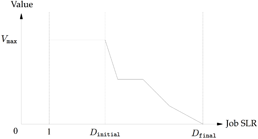
Figure 1: Value Curve Template

$\mathtt{Value}\left(\textrm{job}\;J^{k},\mathtt{SLR}\right)=$

$$\begin{cases}J_{\mathtt{VMax}}^{k}&\mathtt{if\;SLR}\leq D_{\mathtt{initial}}\\ 0&\mathtt{if\;SLR}\geq D_{\mathtt{final}}\\ J_{\mathtt{VMax}}^{k}\times\mathtt{factor}\left(J_{C^{i}}^{k},\>\mathtt{SLR}\right)&\mathtt{if}\;D_{\mathtt{initial}}<\mathtt{SLR}<D_{\mathtt{final}}\end{cases}$$

Algorithm 1 Value Calculation

$\mathtt{factor}\left(\textrm{curve}\;C^{i},\mathtt{SLR}\right):$

$\mathtt{t\_sort=}\left[\mathtt{p}\left[0\right]\mathtt{\>for\>p\>in\>}C^{i}\right]$

$\mathtt{v\_sort=}\left[\mathtt{p}\left[1\right]\mathtt{\>for\>p\>in\>}C^{i}\right]$

$\mathtt{low\_index=}\left|\left[\mathtt{t\>for\>t\>in\>t\_sort\>if\>t}\leq\mathtt{SLR}\right]\right|$

$\mathtt{t\_low=t\_sort}\left[\mathtt{low\_index}\right]$

$\mathtt{t\_high=t\_sort}\left[\mathtt{low\_index}+1\right]$

$\mathtt{v\_low=v\_sort}\left[\mathtt{low\_index}\right]$

$\mathtt{v\_high=v\_sort}\left[\mathtt{low\_index}+1\right]$

$F=\mathtt{v\_low}+\left(\frac{\mathtt{SLR-t\_low}}{\mathtt{t\_high-t\_low}}\times\left(\mathtt{v\_high-v\_low}\right)\right)$

$\mathtt{return}\>F$

Algorithm 2 Value Factor Calculation

IV Bidding Policies

In a market, independent agents need to make bids for the services they require. In this context of market-based scheduling, tasks will each bid for computational resource. In this market, it is necessary to have policies that calculate the bids for the tasks. These bids can be based a number of underlying attributes of the task.

Baseline policies are explicitly intended to be simplistic or naive, to show what is achievable with little processing work. Two baseline policies are considered, Random and First In First Out (FIFO). Random places a random bid for each task in the queue at each round of bidding. FIFO places bids that are proportional to the arrival time of each task’s parent job $T^{i}\in J^{k},\;FIFO=J_{\mathtt{arrive}}^{k}$, with the smallest numerical bid being the highest priority.

Several policies are considered that do not make use of the value curves. These instead use the upward ranks of tasks $T_{R}^{i}$ within the dependency graph of their parent job. Shortest Remaining Time First (SRTF) and Longest Remaining Time First (LRTF) [25, 22] bid for tasks using their upward rank, with the smallest and largest bids being given priority, respectively.

The Projected Schedule Length Ratio (P-SLR) policy bids the P-SLR value, with the highest value being highest priority [3]. This is so that the tasks that are most late relative to their execution time are given the highest priority, which is intended to ensure that all jobs will have a waiting time proportional to the length of their critical path, a desirable attribute for fairness and responsiveness [19]. The P-SLR as defined above is starvation-free as long as overloads are transient (overall load is below 100%). However, to ensure P-SLR is starvation-free under extremely high load, a further term is added to the equation. The equation as used for P-SLR bidding in the simulation is shown in Algorithm 3. One discrete time unit is also added to the P-SLR calculation in order to preferentially prioritise smaller tasks that arrive at the same instant as larger ones.

$\mathtt{projected\_slr}(\textrm{task}\;T^{i},\;\textrm{job\ }\;J^{k},\mathtt{curr\_time},\;\textrm{queue}\;Q)=$

$$\frac{\left(T_{R}^{i}+\mathtt{curr\_time}+1\right)-J_{\mathtt{arrive}}^{k}}{J_{\mathtt{CP}}^{k}}+\left\lfloor\frac{\mathtt{curr\_time}-J_{\mathtt{arrive}}^{k}}{\forall J^{n}\in Q:\max\left(J_{\mathtt{CP}}^{n}\right)}\right\rfloor^{2}$$

Algorithm 3 Projected SLR algorithm

Several policies based on value are considered. Projected Value (PV) uses the estimated P-SLR to determine the parent job’s value if it were to finish after the task’s upward rank. PV then uses the highest bids as the most preferable. This is similar to previous market-based policies where work has fixed values rather than value curves $T^{i}\in J^{k}:\;PV\left(T^{i}\right)=\mathtt{Value}\left(J^{k},\;PSLR\left(T^{i}\right)\right)$.

The issue with PV is that tasks that promise a large amount a value may also take a large amount of resource. Instead, the Projected Value Density (PVD) policy [15] looks at how profitable running each task may be, by comparing the value gained with the resource required to achieve this value. The resource required, $T_{\mathtt{succ\_sum}}^{i}$, is the sum of the execution times, $T_{\mathtt{exec}}^{i}$, multiplied by the cores they require, $T_{\mathtt{cores}}^{i}$, of all the tasks that depend on the considered task $\forall\,T^{j}\in T_{\mathtt{succ}}^{i}:T_{\mathtt{succ\_sum}}^{i}=\left(T_{\mathtt{exec}}^{i}\times T_{\mathtt{cores}}^{i}\right)+\sum T_{\mathtt{succ\_sum}}^{j}$. Having defined the resource required, we can define the value density as the value divided by the resource required $T^{i}\in J^{k}:\;PVD\left(T^{i}\right)=\mathtt{Value}\left(J^{k},\;PSLR\left(T^{i}\right)\right)\div T_{\mathtt{succ\_sum}}^{i}$ . Higher density is prioritised as it will be most profitable.

Aldarmi and Burns [1] suggested that squaring the value density gives a better separation between tasks that will be profitable and those that should be starved to avoid wasting resources. This is termed the Projected Value Density SQuared (PVDSQ) policy, $PVDSQ\left(T^{i}\right)=\left(PVD\left(T^{i}\right)\right)^{2}$.

The Projected Value Remaining (PVR) policy [5] is designed to capture the relative urgency of a task at a given moment. The other policies may project tasks to be valuable or not, but are unable to give an indication of whether that value is likely to decrease with waiting much longer. PVR uses the P-SLR to determine the earliest possible time a task could finish if it were run immediately. The PVR is then the area under the value curve remaining between the P-SLR at the current time and the final deadline $D_{\mathtt{final}}$ of the job. This is illustrated graphically in Figure 2.

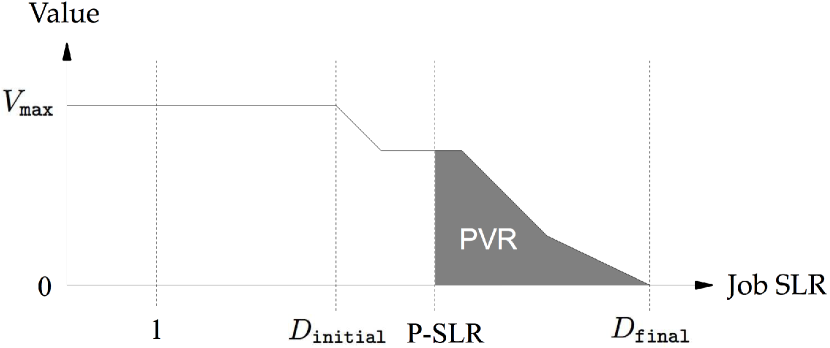
Figure 2: Value Curve showing Projected Value Remaining

The tasks with the smallest value remaining are run first. Urgent tasks would have a steeply sloping value curve, which would give only a small area under the curve. Tasks about to time out would also have only a small area remaining. Prioritising these tasks would reduce starvation and loss of value.

The value curves were designed using linear interpolation between the points so that the definite integral of this curve would be quickly and exactly calculable using the trapezoidal method [2]. However, the policy method generalises to any value curves where value can only decrease over time, as long as a final deadline is present. The algorithm to calculate PVR is given in Algorithm 4.

$\mathtt{PVR}\left(T^{i},\>\mathtt{\tau_{current}}\right):$

$$J^{k} = T_{\mathtt{parent\_job}}^{i}$$

$$D_{\mathtt{final}} = J_{C_{D_{\mathtt{final}}}^{i}}^{k}$$

$$\mathtt{P\_SLR} = \frac{\left(T_{\mathtt{R}}^{i}+\tau_{\mathtt{current}}\right)-J_{\mathtt{arrive}}^{k}}{J_{\mathtt{CP}}^{k}}$$

$$PVR = \int_{\mathtt{P\_SLR}}^{D_{\mathtt{final}}}\mathtt{Value}\left(J^{k},s\right)\>ds$$

$$\mathtt{return} PVR$$

Algorithm 4 Algorithm to compute Projected Value Remaining

V Experimental Method

In order to be able to compare different schedules, appropriate metrics are required. For this work, the pertinent metric is that of the proportion of maximum value achieved. The maximum value of a workload is the sum of the maximum value of all possible jobs, and is the value that would be achievable if the number of processors available was unbounded, there was no contention between work and no network delays. Because different workloads may have different maximum values, it is necessary to normalise these values between workloads. In this work, the value achieved under a given set of circumstances is divided by the maximum possible value to give a normalised figure.

Users are likely to not only care about their work, but also care whether it was completed or not. Therefore the number of jobs starved in a given set of circumstances will also be examined. A job is considered to have starved (and is removed from the queue) once it has passed its final deadline $D_{\mathtt{final}}$ as defined by its value curve.

The bidding policies are evaluated in simulation, using a synthetic workload running over a synthetic platform. The simulations take place within a discrete-time environment, implemented using the SimPy library [20] in the Python language. The platform consists of 4000 cores total, organised into clusters of 1000 cores each. Three clusters are of architecture Kind1, and one of Kind2. The clusters are all connected directly to the central router, where the auction is run. Network delays between the clusters is accounted for by using a Communication to Computation ratio of 0.2.

Ten synthetic workloads were used for evaluation. To ensure sufficient scale was present, each workload was made up of 10,000 jobs with 5-20 tasks per job. This gives approximately 100,000 tasks in each workload. The execution time distribution for jobs and tasks followed a log-uniform distribution. 80% of the tasks in the workload were Kind1, with 20% being of Kind2. The dependencies between jobs followed an exponential distribution in node degree. These synthetic workloads were created using the methods published by Burkimsher et al. [4]. Value curves were also generated synthetically, and had $D_{\mathtt{initial}}$ values randomly selected between 2 and 4, $D_{\mathtt{final}}$ values between 6 and 10, and 5-10 random, non-increasing points in between.

In simulation, real allocations of value are unavailable. Therefore, it was assumed that the value of jobs was proportional to the number of core-minutes their execution would consume. That is, that their value density at $V_{\mathtt{max}}$ is identical. In periods of overload, however, jobs may have very different value densities because the value curves specified will lead to them having very different relative urgency.

Load can be varied for the same workload by adjusting the inter-arrival times of jobs, according to the method in Burkimsher et al. [4]. The arrival rates are also adjusted to give peaks during working hours and quieter periods overnight and at the weekend. This ensures that many cycles of overload and catching-up are present, a more challenging scenario for a scheduler than a constant arrival rate of work and one that is more representative of real systems. Using this method, load is varied between 70% and 140% of saturation, the state where the system must operate at full capacity to service the work arriving. Load above 100% represents overload, where not all the work can be run. With the daily and weekly cycles of load, transient overloads will be present even below 100% total load.

VI Results and Discussion

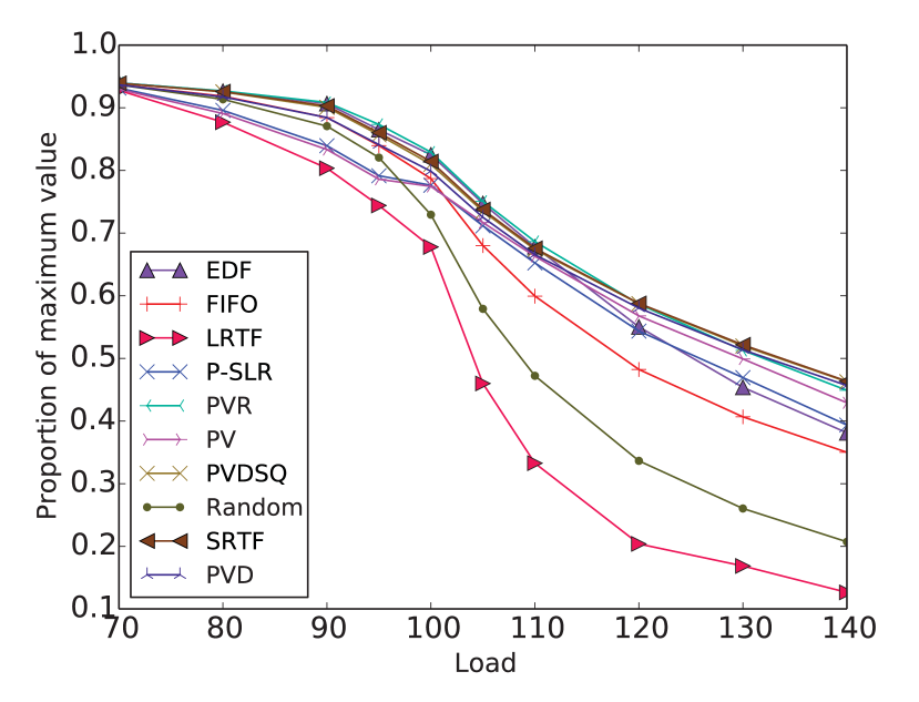
Figure 3: Value against load for different bidding policies

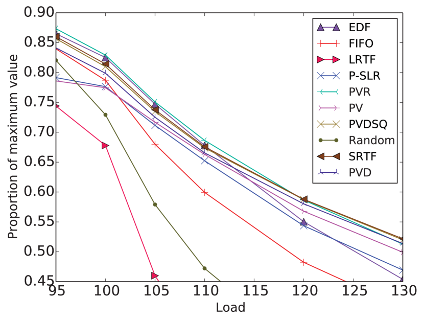
Figure 4: Value against load for different bidding policies (Detail)

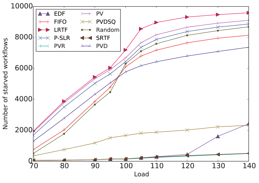
Figure 5: Starvation against load for different bidding policies

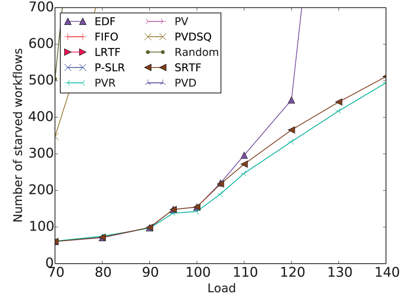
Figure 6: Starvation against load for different bidding policies (Detail)

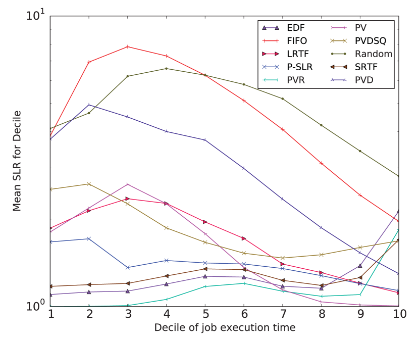
Figure 7: Responsiveness (SLR) across the spectrum of job execution times at 120% load

The experiments were set up such that there will always be transient overloads, so that not all work is able to run. This is why the proportion of maximum value is below 1.0 even at 70% load. As load is increased, the proportion of value decreases for all bidding policies. This is bound to happen because the more work there is to do in a given time, the more there will be that is not done. The challenge is to find the policy that suffers the least loss of value given the increase in load, with the results shown in Figure 3.

LRTF is a policy commonly used in static scheduling as it is good at bin-packing, and hence at reducing workload makespan [22]. However, it is clear that it is a poor choice for a dynamic scheduling scenario, because it will tend to run the most recently arrived jobs first. This is because the jobs most recently arrived will have lots of work left to do, and so be prioritised over those that are soon to finish. In an overload situation, jobs will be started continuously but never be able to finish. Its value achieved in this dynamic case is even worse than the baseline random policy.

The FIFO policy is a fair improvement on the random policy, but FIFO is still a long way behind the other policies under overload. This is natural because it does not consider the size or the relative urgency of jobs.

At load levels below overload, the PV policy performs surprisingly poorly, even worse than the random policy. PV goes for the largest and most valuable tasks first, meaning that many smaller ones will starve. This affects the total value achievable, and it also leads to the most tasks starving across the spectrum of load, with only LRTF starving more. At very high levels of load, PV does not fall as fast as some other policies, though it is still beaten by the flavours of Value Density, SRTF and PVR.

P-SLR is designed to ensure that the SLR of jobs across the execution time spectrum is equal (fairness with respect to responsiveness) [3]. Under high levels of load, however, this can mean that many jobs may have their final deadline before the SLR that is currently being achieved, meaning that many will starve (Figure 5). P-SLR is unable to take into account the fact that jobs may have varying levels of urgency.

The two flavours of value density bidding (PVD and PVDSQ) are clearly better than simply using value-based bidding. Locke [15] showed that for uniprocessor scheduling of workloads that are also schedulable using EDF, value density based scheduling was optimal. Naturally, workloads that overload their platform are not schedulable using EDF, so these scenarios are outside those proved optimal. This evaluation shows that in the overload scenarios considered, other policies can do better than PVD.

Interestingly, PVDSQ gives higher value than PVD (Figure 3). This is because PVDSQ starves many fewer tasks than PVD (Figure 5). By squaring the value density, jobs that are not worth running are more cleanly starved, leaving the rest to be able to run to completion. PVDSQ also starves a few more of the largest jobs, which gives a lot more space for other jobs to run. Interestingly, PVDSQ and SRTF give almost indistinguishable levels of value across the load spectrum. However, SRTF starves many fewer tasks overall because SRTF prioritises small tasks with little time remaining.

EDF attains the second-highest level of value below 110% load (Figure 4). However, its performance falls steeply after that. This is because once the earliest deadline that is being run gets into the past, every job starts missing its deadline and lateness starts cascading. Above 110% load, the value attained by EDF falls rapidly behind the alternative policies evaluated. After 120% load, the number of tasks starved by EDF also increases rapidly (Figure 6).

Below saturation and up to 110% load, PVR attains the highest value of all the policies evaluated. This is due to its ability to take into account the urgency of tasks. Small, urgent tasks are able to run, which ensures their value is captured before they starve. PVR actually has the highest responsiveness (lowest SLR) of all the policies evaluated for smaller jobs (Figure 7). It does this by only letting the largest jobs have their SLR increase. However, the largest jobs can often also be those that are most tolerant to waiting time: if a job takes months to run, it may be able to take a few more days and users will not mind. This means that the value curves are likely to decrease relatively gradually.

At very high levels of load, PVR’s lead is eroded and it falls behind SRTF and PVDSQ and is equalled by PVD at the highest level of load evaluated. When there is too much work to run, PVR tends to keep most jobs running by starving the largest ones. Yet the largest jobs can also be the ones that supply the most value. As can be seen from Figure 7, SRTF penalises the largest jobs a little less, meaning that it keeps more value overall under extreme overload. Saying that, PVR has the lowest number of starved jobs across the spectrum of load (Figure 6). PVR manages to ensure that only 5% of jobs are incomplete by their final deadline, even at 140% load. This low level of starvation is likely to be attractive to grid operators because it will keep user satisfaction high, as no user wishes to have their job starve.

VII Conclusion

In this paper, a number of bidding policies for market-based scheduling in a distributed grid computing scenario were examined. The Projected Value Remaining (PVR) policy was shown to achieve the highest levels of value as long as overload was not excessive. Even under extreme overload, the relatively low levels of starved jobs are likely to be more acceptable to users than the slight improvement in overall value offered by the PVDSQ policy. PVR is also likely to be preferable to SRTF under extreme overload, because most jobs still have high responsiveness, and it is the largest jobs, for which responsiveness is usually less critical anyway because their execution times are so long, that must wait longer. PVR’s ability to capture urgency in its bidding metric is what enables it to give these results.

A further notable conclusion is that the differences between the leading policies are really quite close in terms of the value achieved, even when the number of jobs they starve is wildly different. This evaluation shows that different policies achieve similar levels of value using quite different behaviour. Some policies run just the largest jobs and starve everything else (PV), others the smallest (SRTF), while others try to achieve balance across the space of execution times (EDF, PVDSQ, PVR).

This work considers the scenario where all work is admitted but may be left in the queue to starve. This may be less useful to users than a system with an admission controller. Users could then know up-front whether their jobs were accepted, and find out sooner if their jobs were not going to be run. A natural direction for future work would be to see whether integrating the current approaches with the addition of an admission controller could achieve similar levels of value.

The research described in this paper is partially funded by the EU FP7 DreamCloud Project (611411).

References

- [1] Saud A. Aldarmi and Alan Burns. Dynamic value-density for scheduling real-time systems. In Proceedings of The 11th Euromicro Conference on Real-Time Systems, pages 270–277, June 1999.
- [2] Fernando L. Alvarado. Parallel solution of transient problems by trapezoidal integration. IEEE Transactions on Power Apparatus and Systems, PAS-98(3):1080–1090, 1979.
- [3] Andrew Burkimsher, Iain Bate, and Leandro Soares Indrusiak. A survey of scheduling metrics and an improved ordering policy for list schedulers operating on workloads with dependencies and a wide variation in execution times. Future Generation Computer Systems, 29(8):2009 – 2025, October 2013.
- [4] Andrew Burkimsher, Iain Bate, and Leandro Soares Indrusiak. A characterisation of the workload on an engineering design grid. In Proceedings of the High Performance Computing Symposium, HPC 2014, pages 8:1–8:8, San Diego, CA, USA, 2014. Society for Computer Simulation International.
- [5] Andrew M. Burkimsher. Fair, responsive scheduling of engineering workflows on computing grids, EngD Thesis, University of York, 2014.
- [6] Ken Chen and Paul Muhlethaler. A scheduling algorithm for tasks described by time value function. Real-Time Systems, 10(3):293–312, 1996.
- [7] Nicolas Dube and Marc Parizeau. Utility computing and market-based scheduling: Shortcomings for grid resources sharing and the next steps. In Proceedings of the 22nd International Symposium on High Performance Computing Systems and Applications, 2008, HPCS 2008, pages 59–68, June 2008.
- [8] Ronald L. Graham. Bounds on multiprocessing timing anomalies. SIAM Journal on Applied Mathematics, 17:416–429, 1969.
- [9] Intel Corporation. Enhanced Intel SpeedStep technology for the Intel Pentium M processor - white paper, March 2004.
- [10] David E. Irwin, Laura E. Grit, and Jeffrey S. Chase. Balancing risk and reward in a market-based task service. In Proceedings of the 13th IEEE International Symposium on High Performance Distributed Computing, HPDC 2004, pages 160–169, Washington, DC, USA, 2004. IEEE Computer Society.
- [11] James E. Kelley, Jr. Critical-path planning and scheduling: Mathematical basis. Operations Research, 9(3):pp. 296–320, 1961.
- [12] Carl Kesselman and Ian Foster. The Grid: Blueprint for a New Computing Infrastructure. Morgan Kaufmann Publishers, San Francisco, CA, USA, November 1999.
- [13] Kevin Lai, Lars Rasmusson, Eytan Adar, Li Zhang, and Bernardo A. Huberman. Tycoon: An implementation of a distributed, market-based resource allocation system. Multiagent and Grid Systems, 1(3):169–182, August 2005.
- [14] Chen Lee, John Lehoczky, Dan Siewiorek, Ragunathan Rajkumar, and Jeff Hansen. A scalable solution to the multi-resource QoS problem. In Proceedings of the 20th IEEE Real-Time Systems Symposium (RTSS 1999), pages 315–326, Washington, DC, USA, 1999. IEEE Computer Society.
- [15] Carey Douglass Locke. Best-effort decision-making for real-time scheduling. PhD thesis, Carnegie-Mellon University, Pittsburgh, PA, USA, May 1986.
- [16] Muthucumaru Maheswaran, Tracy D. Braun, and Howard Jay Siegel. Heterogeneous distributed computing. In Encyclopedia of Electrical and Electronics Engineering, pages 679–690. John Wiley, 1999.
- [17] Mark S. Miller and K. Eric Drexler. Markets and computation: Agoric open systems. In B. A. Huberman, editor, The Ecology of Computation, pages 133–176, Amsterdam, 1988. North-Holland Publishing Company.
- [18] Florentina I. Popovici and John Wilkes. Profitable services in an uncertain world. In Proceedings of the ACM/IEEE SC 2005 Conference on Supercomputing, pages 36–36, November 2005.
- [19] Erik Saule, Doruk Bozdağ, and Umit V. Catalyurek. A moldable online scheduling algorithm and its application to parallel short sequence mapping. In Eitan Frachtenberg and Uwe Schwiegelshohn, editors, Job Scheduling Strategies for Parallel Processing, volume 6253 of Lecture Notes in Computer Science, pages 93–109. Springer Berlin Heidelberg, 2010.
- [20] Team SimPy. Welcome to simpy, 2015.
- [21] Ivan Edward Sutherland. A futures market in computer time. Communications of the ACM, 11(6):449–451, June 1968.
- [22] Haluk Topcuouglu, Salim Hariri, and Min-You Wu. Performance-effective and low-complexity task scheduling for heterogeneous computing. IEEE Transactions on Parallel and Distributed Systems, 13(3):260–274, March 2002.
- [23] William Voorsluys, James Broberg, and Rajkumar Buyya. Cloud Computing: Principles and Paradigms, chapter Introduction to Cloud Computing, pages 1–44. Wiley Press, New York, USA, February 2011.
- [24] Carl A. Waldspurger, Tad Hogg, Bernardo A. Huberman, Jeffrey O. Kephart, and W. Scott Stornetta. Spawn: a distributed computational economy. IEEE Transactions on Software Engineering, 18(2):103–117, February 1992.
- [25] Henan Zhao and Rizos Sakellariou. Scheduling multiple DAGs onto heterogeneous systems. In Proceedings of the 20th International Parallel and Distributed Processing Symposium (IPDPS), 2006.