Optimal performance of heat engines with a finite source or sink
and inequalities between means

Abstract

Given a system with a finite heat capacity and a heat reservoir, and two values of initial temperatures, $T_{+}$ and $T_{-}(<T_{+})$, we enquire, in which case the optimal work extraction is larger: when the reservoir is an infinite source at $T_{+}$ and the system is a sink at $T_{-}$, or, when the reservoir is an infinite sink at $T_{-}$ and the system acts as a source at $T_{+}$? It is found that in order to compare the total extracted work, and the corresponding efficiency in the two cases, we need to consider three regimes as suggested by an inequality, the so-called arithmetic mean-geometric mean inequality, involving the arithmetic and the geometric means of the two temperature values $T_{+}$ and $T_{-}$. In each of these regimes, the efficiency at total work obeys certain universal bounds, given only in terms of the ratio of initial temperatures. The general theoretical results are exemplified for thermodynamic systems for which internal energy and temperature are power laws of the entropy. The conclusions may serve as benchmarks in the design of heat engines, where we can choose the nature of the finite system, so as to tune the total extractable work and/or the corresponding efficiency.

I I. Introduction

Thermodynamics is regarded as a discipline with a formal simplicity, but still covering a wide domain of applicability. One of the central problems in thermodynamics is the extent of heat-to-work conversion, with its focus on maximal work or power output and the consequent efficiency of the process. The seminal results of Carnot apply to the case of infinite reservoirs. However, in recent years, the study of the role of finite reservoirs has also caught attention Ondrechen et al. (1981, 1983); Leff (1987); Yan and Chen (1997); Izumida and Okuda (2014); Wang (2014); Johal and Rai (2016). This is motivated by practical considerations such as a limited supply of fuel (a finite heat source), or the working medium being in contact with a small environment (sink) which may be the case in small-scale devices, or even relevant for the design of modern cities.

On the other hand, algebraic inequalities between the means hold a kind of poetic fascination. One of the most important Alsina and Nelson (2009) and well-known is the arithmetic mean-geometric mean (AM-GM) inequality, stated as follows. For two real positive numbers, $a$ and $b$, with arithmetic mean $A(a,b)=(a+b)/2$ and geometric mean $G(a,b)=\sqrt{ab}$, we have

$$\frac{a+b}{2}\geqslant\sqrt{ab},$$ (1)

with equality only if $a=b$. Such inequalities are useful in proving elementary results in many disciplines Hardy et al. (1952); Bullen et al. (1988). Especially, in the context of macroscopic thermodynamics, the second law of increase of entropy may be argued as follows Cashwell and Everett (1967). Consider $n$ systems with a constant heat capacity $C$ and initial temperatures, $\{T_{i}|i=1,...,n\}$. Placed in mutual thermal contact, these systems come to equilibrium at a common final temperature, say $T_{f}$. From the energy conservation condition (the first law), we have $\sum_{i}C(T_{i}-T_{f})=0$, which implies $T_{f}=\sum_{i}T_{i}/n$. Now the total entropy change: $\Delta S=\sum_{i}\int_{T_{i}}^{T_{f}}(C/T)dT=nC(\ln T_{f}-\ln(\Pi_{i}T_{i})^{1/n})$, so by virtue of the AM-GM inequality gen , we get $\Delta S\geqslant 0$ com ; Tait (1868); Sommerfeld (1956); Landsberg and Pečarić (1987). Thus in the above argument, the manifestation of AM-GM inequality is specifically tied to the assumption of a particular model system. By assuming systems other than perfect gases, one can invoke inequalities between other means.

It is apparent that alternative thermodynamic processes, such as optimal work-extracting processes, would exhibit a similar connection between physical models and specific inequalities between the means. In this paper, our objective is to compare the work output capacity and efficiency of two complementary scenarios, involving a finite system and a reservoir. During this analysis, we will uncover a rather general role of the AM-GM inequality. In particular, we will address the following question. Assume a pair of values for temperature, say $T_{+}$ and $T_{-}(<T_{+})$, and a system A with a finite heat capacity. Also, a heat reservoir is present such that if the system is at temperature $T_{+}$, the reservoir is a sink at $T_{-}$. Conversely, if the system is at $T_{-}$, then the reservoir is a hot source at $T_{+}$. Which of these two situations (see Fig. 1) would yield a larger amount of extractable work, due to temperature difference? We answer this question by assuming that the process of maximal work extraction is carried out by some working medium (whose details are not important) via infinitesimal reversible heat cycles between system A and the reservoir.

In practical terms, we may consider a toy engine which can ideally work in a reversible manner, utilizing the temperature gradient between system A and the environment. Let $T_{+}$ and $T_{-}$ be the environment temperatures, say, in summer and in winter season, respectively. So in summer, we cool the system A to temperature $T_{-}$, while in winter, we have to heat up the system to temperature $T_{+}$, in order to run the engine. The engine works till it equilibrates at the specific temperature of the environment. When will the engine yield a larger amount of total work, in summer, or in winter?

The paper is organized as follows. In Section II, we describe the framework using two scenarios for work extraction due to temperature difference between a finite system and a heat reservoir. In Subsection II.A, the total extracted work and the corresponding efficiency are compared for the two scenarios. In Section III, physical examples are given based on thermodynamic systems where the temperature and the internal energy are related to the entropy by power laws. Section IV discusses the bounds on the efficiency at total work. Finally, Section V is devoted to summary and concluding remarks.

II II. Work from a finite system and a reservoir

To set up the thermodynamic framework, consider system A following a certain fundamental relation $U=U(S,V,N)$. It has equilibrium states described by energy $U_{+}$, entropy $S_{+}$ at temperature $T_{+}$, and alternatively, by $U_{-}$ and $S_{-}$ at $T_{-}$, with some fixed values of volume $V$ and number of moles $N$. For simplicity, we consider only systems with a positive heat capacity ($C_{V}>0$). This implies that $U_{+}>U_{-}$ and $S_{+}>S_{-}$.

Now, we first assume that system A acts as a finite heat sink at temperature $T_{-}$, relative to a very large hot reservoir (source) at temperature $T_{+}$. We couple the two by running infinitesimal heat cycles, which successively increase the temperature of A, till A comes in equilibrium with the hot source, see Fig.1 (i). At an arbitrary intermediate stage, when the temperature of A is $T$, the small amount of heat removed from the source $dQ_{h}$ is converted into an amount of work $dW$ with maximal (Carnot) efficiency $\eta=1-T/T_{+}$. The heat discarded to the sink is $dQ_{c}=C_{V}dT$. Then, we can write $dW=\eta(1-\eta)^{-1}dQ_{c}$. The total extracted work is given by:

$$W_{+} = \int_{T_{-}}^{T_{+}}dW$$ (2)

$$= \int_{T_{-}}^{T_{+}}\frac{\eta}{1-\eta}C_{V}dT$$ (3)

$$= T_{+}(S_{+}-S_{-})-(U_{+}-U_{-}).$$ (4)

The heat absorbed from the hot source is $Q_{+}=T_{+}(S_{+}-S_{-})$. Then the efficiency at total work, $\eta_{+}=W_{+}/Q_{+}$, is calculated to be:

$$\eta_{+}=1-\frac{1}{T_{+}}\frac{U_{+}-U_{-}}{S_{+}-S_{-}}.$$ (5)

Then, we consider the alternative situation in which A acts as a finite source at temperature $T_{+}$, relative to an infinite sink at $T_{-}$, see Fig.1 (ii). Again, we extract the maximal work by utilizing the temperature gradient between A and the reservoir, till A is at temperature $T_{-}$. Then, after a similar calculation Izumida and Okuda (2014) as above, the total work obtained is

$$W_{-}=(U_{+}-U_{-})-T_{-}(S_{+}-S_{-}).$$ (6)

This is termed as exergy in the engineering literature Moran et al. (2010). The heat absorbed from the source is $Q_{-}=U_{+}-U_{-}$, while the efficiency of the process $\eta_{-}=W_{-}/Q_{-}$ is given by

$$\eta_{-}=1-T_{-}\frac{S_{+}-S_{-}}{U_{+}-U_{-}}.$$ (7)

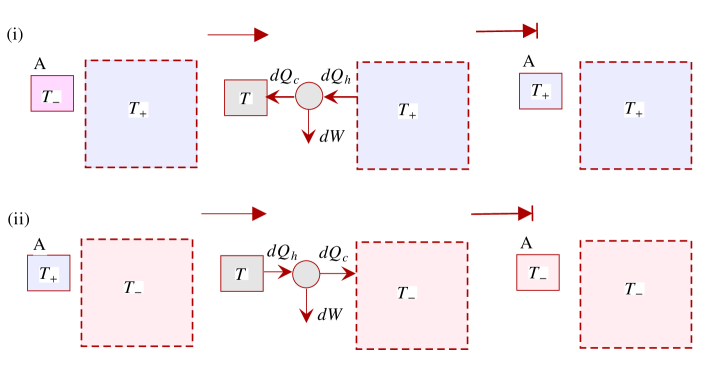
Figure 1: Schematic of the reversible heat engine between a finite system and a heat reservoir, for a given pair of initial temperatures $(T_{+},T_{-})$: (i) System A is a finite sink at $T_{-}$ and is coupled to an infinite source at $T_{+}$, via heat engine. Work extraction $W_{+}$, Eq. (4), is completed when the temperature of A becomes $T_{+}$. (ii) System A is a finite source at $T_{+}$ and is coupled to an infinite sink at $T_{-}$, via heat engine. Total extracted work is $W_{-}$, Eq. (6), when the temperature of A becomes $T_{-}$.

Thus for the toy engine mentioned in Introduction, $W_{+}$ and $\eta_{+}$ ($W_{-}$ and $\eta_{-}$) may refer to the total work and the corresponding efficiency in summer (winter) season.

II.1 A. The Comparison

Now we compare the amounts of extracted work, and the efficiencies, in these alternative set-ups. For that purpose, we recall the classic result in calculus, known as the mean value theorem. Consider a continuous and differentiable function $U(S)$ in the domain $[S_{-},S_{+}]$, with the derivative $T(S)=dU/dS$. Let us denote: $U(S_{\pm})=U_{\pm}$. Following the theorem, there is a point $S_{m}$ strictly within this interval ($S_{+}>S_{m}>S_{-}$), at which the derivative of the function $U$, i.e. $T(S_{m})\equiv T_{m}$, is given by:

$$T_{m}=\frac{U_{+}-U_{-}}{S_{+}-S_{-}}.$$ (8)

We also assume $T(S)$ to be monotonic increasing function, or, in other words, $U(S)$ is a convex function. In the context of thermodynamics, this assumption implies positive heat capacity ($C_{V}$) of the system. Then it follows that $T(S_{+})>T(S_{m})>T(S_{-})$, or alternatively, $T_{+}>T_{m}>T_{-}$.

Now, depending on the nature of the thermodynamic system i.e. the form of the function $U(S)$, $T_{m}$ can take values relative to $A(T_{+},T_{-})$ and $G(T_{+},T_{-})$, such that we have the following situations:

$$(a)\qquad\qquad T_{+} > T_{m}\geqslant\frac{T_{+}+T_{-}}{2}>\sqrt{T_{+}T_{-}}>T_{-}$$

$$(b)\qquad\qquad T_{+} > \frac{T_{+}+T_{-}}{2}>T_{m}>\sqrt{T_{+}T_{-}}>T_{-}$$

$$(c)\qquad\qquad T_{+} > \frac{T_{+}+T_{-}}{2}>\sqrt{T_{+}T_{-}}\geqslant T_{m}>T_{-}$$

We choose the means $A$ and $G$ to split the interval $(T_{-},T_{+})$ into three regions, because for $T_{m}=(T_{+}+T_{-})/2$, we have $W_{+}=W_{-}$, and for $T_{m}=\sqrt{T_{+}T_{-}}$, we have $\eta_{+}=\eta_{-}$. This helps naturally to compare the magnitudes of work, and efficiency. Thus, if case $(a)$ holds, then applying $T_{m}\geqslant(T_{+}+T_{-})/2$, and using Eqs. (8), (4) and (6), we obtain $W_{+}\leqslant W_{-}$. In this case, due to AM-GM inequality, we also have $T_{m}>\sqrt{T_{+}T_{-}}$, which implies $\eta_{+}<\eta_{-}$, due to Eqs. (8), (5) and (7).

Similarly, if case $(b)$ applies, then we conclude that $W_{+}>W_{-}$, but due to AM-GM inequality, we have $\eta_{+}<\eta_{-}$. If case $(c)$ is true, i.e. $\sqrt{T_{+}T_{-}}\geqslant T_{m}$, it implies $\eta_{+}\geqslant\eta_{-}$. Further, due to $(T_{+}+T_{-})/2>T_{m}$, we also have $W_{+}>W_{-}$. The above three scenarios are summarized in Table I.

Thus we see that the comparison of $T_{m}$ with $A(T_{+},T_{-})$ decides the relative magnitudes of $W_{+}$ and $W_{-}$, whereas the comparison of $T_{m}$ with $G(T_{+},T_{-})$, serves to compare $\eta_{+}$ and $\eta_{-}$. In these comparisons, the AM-GM inequality provides a sort of background against which $T_{m}$ takes values depending on the nature of system A (see examples below). In terms of practical utility, the goal behind modelling of heat engines is to characterize their optimal working regimes. In this regard, if we are given a finite system A and a constraint to run the engine in one of the two scenarios, denoted as (i) and (ii) in the above, then a particular choice can be motivated as follows. In case the system A falls in category (a) of Table I, then choice (ii) provides a higher total work output and a higher efficiency. On the other hand, if system A belongs to category (c), then the choice (i) would provide a higher work output and a higher efficiency. In case the system belongs to regime (b), we have a situation with a trade-off. If we opt for a higher work output then the efficiency obtained is less, and vice versa. Heuristically, one may be able to make a choice in this situation as follows. A focus on a higher efficiency may become important, if the substance (system A) is in short supply or if the economic/ecological costs of preparing the system, in the desired state, are rather high. On the other hand, if such costs are not a consideration, then one may focus on higher total work, with the corresponding efficiency being less of a concern.

$(a)$	$(b)$	$(c)$
$W_{+}\leqslant W_{-}$	$W_{+}>W_{-}$	$W_{+}>W_{-}$
$\eta_{+}<\eta_{-}$	$\eta_{+}<\eta_{-}$	$\eta_{+}\geqslant\eta_{-}$

Table 1: Comparison of total work, Eqs. (4) and (6), and efficiency at total work, Eqs. (5) and (7), corresponding to regimes $(a),(b)$ and $(c)$ in Eq. (LABEL:abc).

III III. Examples

In this section, we illustrate the various cases noted in the above, by taking examples from different types of physical systems. Consider a class of thermodynamic systems that obey: $U\propto S^{\omega}$ and $T\propto S^{\omega-1}$, where $\omega$ is a constant real number. For heat capacity to be positive, we must have $\omega>1$. So, $T_{m}$ is evaluated to be:

$$T_{m}=\frac{1}{\omega}\frac{T_{+}^{\omega/(\omega-1)}-T_{-}^{\omega/(\omega-1)}}{T_{+}^{1/(\omega-1)}-T_{-}^{1/(\omega-1)}}.$$ (10)

It is convenient to introduce the generalized mean Stolarsky (1975); Alzer (1987) of two real, positive numbers $(a,b)$:

$$E_{r}(a,b)=\frac{r-1}{r}\frac{a^{r}-b^{r}}{a^{r-1}-b^{r-1}}.$$ (11)

In our case, $T_{m}=E_{r}(T_{+},T_{-})$ with $r=\omega/(\omega-1)$. For $r=2\;(\omega=2)$, $E_{2}(T_{+},T_{-})=(T_{+}+T_{-})/2$. For $r=1/2$ $(\omega=-1)$, $E_{1/2}(T_{+},T_{-})=\sqrt{T_{+},T_{-}}$. Since $E_{r}(a,b)$ is increasing in parameter $r$ Yang and Cao (1989), it follows that, for $r\geqslant 2$ or $\omega\geqslant 2$, we have $T_{m}=E_{r}(T_{+},T_{-})\geqslant E_{2}(T_{+},T_{-})$, which implies $T_{m}\geqslant(T_{+}+T_{-})/2$, or case $(a)$. Therefore, for $2>\omega>1$, the system corresponds to case $(b)$.

Some examples of physical systems in the above class, for appropriate values of $T_{+}$ and $T_{-}$, are: $\omega=4/3$ (black-body radiation), $\omega=5/3$ (degenerate Bose gas) and $\omega=2$ (ideal Fermi gas). The case of a perfect-gas system, can be discussed as the limit $r\to 1$, which yields $E_{1}(T_{+},T_{-})=L(T_{+},T_{-})$, known as the logarithmic mean Carlson (1972); Bhatia (2008):

$$L(T_{+},T_{-})=\frac{T_{+}-T_{-}}{\ln T_{+}-\ln T_{-}}.$$ (12)

Logarithmic mean temperature difference is a useful measure of the effectiveness with which a heat exchanger can transfer heat energy Kay and Nedderman (1985). This mean satisfies:

$$\frac{T_{+}+T_{-}}{2}>L(T_{+},T_{-})>\sqrt{T_{+}T_{-}}.$$ (13)

So if $T_{m}=L(T_{+},T_{-})$, then due to the above inequality, we have an instance of case $(b)$. Thus with a perfect-gas system, the finite-sink/infinite-source setup produces more work than finite-source/infinite-sink setup ($W_{+}>W_{-}$), although the efficiency at total work follows the reverse order ($\eta_{+}<\eta_{-}$).

As our final model system, let A consist of $N$ non-interacting, localized spin-1/2 particles Pathria (1996). Each particle can be regarded as a two-level system, with energy levels ($0$, $\epsilon$). The mean energy for this system, in the limit of high temperatures such that $\epsilon\ll kT$, on keeping terms only upto $(\epsilon/kT)^{2}$, can be approximated as: $U\approx N({\epsilon}/{2}-{\epsilon^{2}}/{4kT})$, with entropy $S\approx Nk(\ln 2-{\epsilon^{2}}/{8k^{2}T^{2}})$. Then from Eq. (8), we have: $T_{m}=2T_{+}T_{-}/(T_{+}+T_{-})$, which is the well-known harmonic mean $H(T_{+},T_{-})$. This mean is strictly less than $G(T_{+},T_{-})$, and thus our spins-system lies in regime $(c)$.

IV IV. Bounds on efficiency

So far, we have noted the comparison between work characteristics for the two given scenarios. In the following, we point out that within a given scenario, the efficiency at total extracted work obeys definite bounds, which are specific to each of the regimes $(a),(b)$ and $(c)$. Thus if $T_{m}\geqslant(T_{+}+T_{-})/2$, then we get from Eq. (5), $\eta_{+}\leqslant\eta_{C}/2$ where $\eta_{C}=1-T_{-}/T_{+}$ is the Carnot limit. Also from Eq. (5), we get $\eta_{-}\geqslant\eta_{C}/(2-\eta_{C})$. Similarly, in regime (c), when $T_{m}\leqslant\sqrt{T_{+}T_{-}}$, we get $\eta_{+}\geqslant\eta_{CA}$ and $\eta_{-}\leqslant\eta_{CA}$, where $\eta_{CA}=1-\sqrt{T_{-}/T_{+}}$ Chambadal (1957); Novikov (1958), which is popularly known as CA-efficiency, after F. L. Curzon and B. Ahlborn who rediscovered this formula Curzon and Ahlborn (1975), see also Vaudrey et al. (2014). These comparative bounds are summarized in Table II, as well as they are depicted in Figs. 2 and 3. Note that the efficiencies $\eta_{C}/2$, $\eta_{CA}$ and $\eta_{C}/(2-\eta_{C})$ are frequently discussed in the context of maximum power output in finite-time models Van den Broeck (2005); Chambadal (1957); Novikov (1958); Curzon and Ahlborn (1975); Esposito et al. (2010). But we observe that, here, within a quasi-static framework, $\eta_{CA}$ serves to separate $\eta_{+}$ and $\eta_{-}$ in regimes $(b)$ and $(c)$.

$(a)$	$(b)$	$(c)$
$0<\eta_{+}\leqslant\eta_{C}/2$	$\eta_{C}/2<\eta_{+}<\eta_{CA}$	$\eta_{CA}\leqslant\eta_{+}<\eta_{C}$
$\frac{\eta_{C}}{2-\eta_{C}}\leqslant\eta_{-}<\eta_{C}$	$\eta_{CA}<\eta_{-}<\frac{\eta_{C}}{2-\eta_{C}}$	$0<\eta_{-}\leqslant\eta_{CA}$

Table 2: The bounds obeyed by efficiencies at total extracted work, $\eta_{+}$ and $\eta_{-}$, in respective regimes given in Eq. (LABEL:abc), where $\eta_{C}=1-T_{-}/T_{+}$ and $\eta_{CA}=1-\sqrt{T_{-}/T_{+}}$.

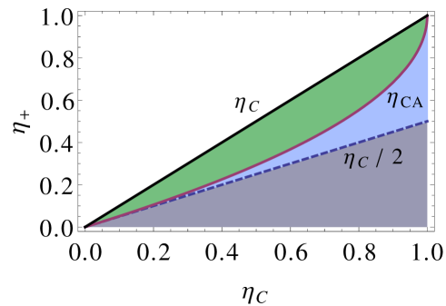
Figure 2: Bounds on efficiency $\eta_{+}$, in the regimes (from bottom to top) $(a),(b)$, and $(c)$, as given in Table II.

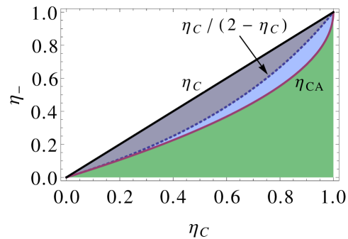
Figure 3: Bounds on efficiency $\eta_{-}$, in the regimes (from top to bottom) $(a),(b)$, and $(c)$, as in Table II.

The above bounds are universal as they depend only on the ratio of the initial temperatures. Note that the actual expressions, (5) and (7), do depend, in general, on the nature of system A. But close to equilibrium, even the general expressions for $\eta_{+}$ and $\eta_{-}$ exhibit a universality. Thus assuming linear response, we can expand energy upto second order in the entropy difference $\delta S=S_{+}-S_{-}$ Johal and Rai (2016):

$$U(S_{-})=U(S_{+})-T_{+}\delta S+\frac{1}{2}\left.\frac{dT}{dS}\right|_{S=S_{+}}(\delta S)^{2}.$$ (14)

Using the above expansion in Eq. (8), and upon simplifying, we get $T_{m}=(T_{+}+T_{-})/2$. This implies that $W_{+}=(T_{+}-T_{-})\delta S/2=W_{-}$. Thus, under linear response, the extracted work is same in both the cases. However, the efficiency at total work is approximated as $\eta_{+}=\eta_{C}/2$ and $\eta_{-}={\eta_{C}}/(2-\eta_{C})$. These expressions are consistent with the findings of Ref. Johal and Rai (2016), where the lower and the upper bounds for efficiency with unequal-sized source and sink, obey the same expressions.

V V. Concluding remarks

We close this investigation by making a few remarks. Apart from an entropy-conserving process, we may analyze an energy-conserving process. The initial and final situations are the same as (i) and (ii) in Fig.1. Specifically, for situation (i), an amount of heat energy $U_{+}-U_{-}$ is removed quasi-statically from the reservoir and deposited in the same manner with the cold system. The change in entropy of system A is $(S_{+}-S_{-})>0$. The change in entropy of the reservoir is: $-(U_{+}-U_{-})/T_{+}$. Thus the total change in the entropy of the universe is:

$$\Delta S_{+}=(S_{+}-S_{-})-\frac{U_{+}-U_{-}}{T_{+}}.$$ (15)

Similarly, if we consider situation (ii), we can conclude that the total entropy change of the universe, in an energy-conserving process, would be:

$$\Delta S_{-}=-(S_{+}-S_{-})+\frac{U_{+}-U_{-}}{T_{-}}.$$ (16)

Now, if we wish to compare the entropy production in the above two cases, then we are led to consider the following situations:

$$(a^{\prime})\qquad\qquad T_{+} > T_{m}\geqslant\frac{2T_{+}T_{-}}{T_{+}+T_{-}}>T_{-}$$

$$(b^{\prime})\qquad\qquad T_{+} > \frac{2T_{+}T_{-}}{T_{+}+T_{-}}>T_{m}>T_{-}.$$ (17)

It is easy to see that if case $(a^{\prime})$ is true, then $\Delta S_{-}\geqslant\Delta S_{+}$. The inverse inequality is valid, if case $(b^{\prime})$ holds. Thus for an energy-conserving process, we see that the inequality between generalized mean $T_{m}$, and $H(T_{+},T_{-})$, quantifies the relative magnitudes of $\Delta S_{-}$ and $\Delta S_{+}$.

Finally, we consider an interesting meaning of $T_{m}$, given by Eq. (8), in the sense of an effective temperature. Take two heat reservoirs with temperatures $T_{m}$ and $T_{-}(<T_{m})$. Let $Q_{m}=U_{+}-U_{-}$, be the heat extracted by the working medium from the hot reservoir in a reversible cycle. Here $U_{\pm}$ refer to the energies of the working medium. Then the change in entropy of the hot reservoir is $T_{m}Q_{m}=S_{+}-S_{-}$. The total extractable work in a reversible cycle is then $(T_{m}-T_{-})(S_{+}-S_{-})$, which is the same as $W_{+}$ in Eq. (6). The Carnot efficiency of this process is $\eta_{m}=1-T_{-}/T_{m}$, which is Eq. (7). A similar conclusion follows for the other scenario, when we consider two heat reservoirs at temperatures $T_{+}$ and $T_{m}(<T_{+})$. Thus $T_{m}$ serves as the effective temperature of one of the two heat reservoirs in an equivalent reversible cycle, which extracts the same amount of work and with the same (Carnot) efficiency.

Concluding, the main focus of this paper was the comparison of performance of a reversible heat engine operating between a finite system and an infinite reservoir, by switching the role of the source and the sink. We compared the total extracted work in the two cases, and the corresponding efficiency of the engine at those values of the work. Interestingly, we find that the conditions for comparison are determined by basic mathematical inequalities between the means, in particular the AM-GM inequality. The present instance of this inequality does not depend specifically on the nature of the system as was the case in earlier studies. The efficiency at total work is naturally split into three regimes, based on this inequality. The bounds separating these regimes are variously given as $\eta_{C}/2$, $\eta_{CA}$ and $\eta_{C}/(2-\eta_{C})$. This highlights a new significance of these expressions for efficiency, which are usually discussed in regard to power output optimization in finite-time models. The utility of our conclusions may also be discussed in the context of the toy engine mentioned in the Introduction. Thus, for a given pair of temperatures $(T_{+},T_{-})$, we can characterize system A, or our device, based on the regime $(a),(b)$ or $(c)$, to which it corresponds. This determines how $W_{+}$ and $W_{-}$ compare with each other, which further guides whether $\eta_{+}$ will be greater, or lesser, relative to $\eta_{-}$. Moreover, in a particular regime, we know from Table II, the bounds within which the efficiency at total work is located. Thus given a choice of system A, the efficiency at total work is restricted within a certain range. Although derived for quasi-static processes, these bounds may serve as benchmarks for tuning the performance of real devices, and can be a useful element in their design.

One of the limitations of our analysis may be that we have considered idealized quasi-static processes. In practical cases, the engines and other thermodynamic machines work in finite cycle-times. Thus an extension of our analysis within an irreversible framework Izumida and Okuda (2014) may help to see how the above conclusions are retained or modified in finite-time models, at least under linear response or beyond that Johal and Rai (2016). Another interesting line of enquiry seems to be the connection of the bounds on efficiency with the principles of inductive inference Johal et al. (2015); Thomas and Johal (2015). Finally, it is hard to ignore the aesthetic motivation in revealing other inequalities, possibly new, with these investigations. But, this is left for future work.

VI Acknowledgements

The author wishes to thank Dr. Renuka Rai, for discussions, and Jannat, for sparing her blackboard.

References

- Ondrechen et al. (1981) M. J. Ondrechen, B. Andresen, M. Mozurkewich, and R. S. Berry, Am. J. Phys. 49, 681 (1981).
- Ondrechen et al. (1983) M. J. Ondrechen, M. H. Rubin, and Y. B. Band, J. Chem. Phys. 78, 4721 (1983).
- Leff (1987) H. S. Leff, Am. J. Phys. 55, 701 (1987).
- Yan and Chen (1997) Z. Yan and L. Chen, J. Phys. A: Math. Gen. 30, 8119 (1997).
- Izumida and Okuda (2014) Y. Izumida and K. Okuda, Phys. Rev. Lett. 112, 180603 (2014).
- Wang (2014) Y. Wang, Phys. Rev. E 90, 062140 (2014).
- Johal and Rai (2016) R. S. Johal and R. Rai, EPL (Europhys. Lett.) 113, 10006 (2016).
- Alsina and Nelson (2009) C. Alsina and R. Nelson, When Less is More: Visualizing Basic Inequalities (The Mathematical Association of America, Washington D.C., 2009) chap.1, page 7.
- Hardy et al. (1952) G. H. Hardy, J. E. Littlewood, and G. Pólya, Inequalities (Cambridge University Press, Cambridge, 1952).
- Bullen et al. (1988) P. S. Bullen, D. S. Mitrinovic, and P. M. Vasić, Means and Their Inequalities (Reidel, Dordrecht, 1988).
- Cashwell and Everett (1967) E. D. Cashwell and C. J. Everett, Am. Math. Monthly 74, 271 (1967).
- (12) For real positive numbers , AM-GM inequality is: .
- (13) An alternate argument presupposes the truth of the second law (), and infers the mathematical inequalities consistent with this assumption. It has been discussed at various times by different authors, see Tait (1868), Sommerfeld (1956), and Landsberg and Pečarić (1987) with references therein .
- Tait (1868) P. G. Tait, Proc. R. Soc. Edinburgh 6, 309 (1868).
- Sommerfeld (1956) A. Sommerfeld, Thermodynamics and Statistical Mechanics, Lectures on Theoretical Physics Vol. V (Academic Press, New York, 1956) problem I.4(b), page 347.
- Landsberg and Pečarić (1987) P. T. Landsberg and J. E. Pečarić, Phys. Rev. A 35, 4397 (1987).
- Moran et al. (2010) M. J. Moran, H. N. Shapiro, D. D. Boettner, and M. B. Bailey, Fundamentals of Engineering Thermodynamics, 7th ed. (Wiley, New York, 2010) chap. 7.
- Stolarsky (1975) K. B. Stolarsky, Math. Mag. 48, 87 (1975).
- Alzer (1987) H. Alzer, Int. J. Math. Educat. Sci. Tech. 20, 186 (1987).
- Yang and Cao (1989) R. Yang and D. Cao, J. Ningbo Univ. 2, 105 (1989).
- Carlson (1972) B. C. Carlson, Am. Math. Monthly 79, 615 (1972).
- Bhatia (2008) R. Bhatia, Resonance 13, 583 (2008).
- Kay and Nedderman (1985) J. M. Kay and R. M. Nedderman, Fluid Mechanics and Transfer Processes (Cambridge University Press, Cambridge, 1985).
- Pathria (1996) R. K. Pathria, Statistical Mechanics (Butterworth-Heinemann, 1996).
- Chambadal (1957) P. Chambadal, Armand Colin, Paris, France 4, 1 (1957).
- Novikov (1958) I. Novikov, J. Nucl. Energy II 7, 125 (1958).
- Curzon and Ahlborn (1975) F. L. Curzon and B. Ahlborn, Am. J. Phys. 43, 22 (1975).
- Vaudrey et al. (2014) A. Vaudrey, F. Lanzetta, and M. Feidt, J. Noneq. Therm. 39, 199 (2014).
- Van den Broeck (2005) C. Van den Broeck, Phys. Rev. Lett. 95, 190602 (2005).
- Esposito et al. (2010) M. Esposito, R. Kawai, K. Lindenberg, and C. Van den Broeck, Phys. Rev. Lett. 105, 150603 (2010).
- Johal et al. (2015) R. S. Johal, R. Rai, and G. Mahler, Found. Phys. 45, 158 (2015).
- Thomas and Johal (2015) G. Thomas and R. S. Johal, Journal of Physics A: Mathematical and Theoretical 48, 335002 (2015).