The slow expansion with nonminimal derivative coupling and its conformal dual

Abstract

We show that the primordial gravitational wave with scale-invariant spectrum might emerge from a nearly Minkowski space, in which the gravity is asymptotic-past free. We illustrate it with a model, in which the derivative of background scalar field nonminimally couples to gravity. We also show that since here the tensor perturbation is dominated by its growing mode, mathematically our slowly expanding background is conformally dual to the matter contraction, but there is no the anisotropy problem.

I Introduction

The inflation paradigm is still the leading candidate of the primordial universe, since it has elegantly solved several problems of the hot big-bang cosmology [1][2][3][4]. Maybe more attractively, inflation can generate primordial perturbations, which give a natural explanation for the origin of the large scale structure and the CMB fluctuations. The nearly scale-invariant, adiabatic, and Gaussian primordial curvature perturbation predicted by slow-roll inflation is consistent with the recent observations, such as Planck [5], see also recent comments [6][7], while the detection of primordial tensor perturbations [8][9], i.e., the primordial gravitational waves (GWs), is still on the road. However, inflation also suffers from the geodesic incompletion problem [10].

During inflation, the parameter $|\epsilon|=|{\dot{H}}|/H^{2}\ll 1$. The evolution with $\epsilon\ll-1$ is called the slow expansion, which may be asymptotically Minkowski in infinite past. It was observed in [11] that such a spacetime might be responsible for adiabatically producing the scale-invariant curvature perturbation, which was implemented ghost-freely in [12][13]. This actually suggests a scenario in which the scale-invariant adiabatic perturbation may emerge from nearly flat Minkowski spacetime. The similar idea was also proposed by Wetterich [14][15] for different motivation. The scale-invariant curvature perturbations can also be obtained during the slow contraction ($\epsilon\gg 1$), i.e., in ekpyrotic universe [16][17], by applying adiabatic ekpyrosis mechanism [18][19], though for ekpyrotic universe the entropic mechanism is actually better to explain the observation [20][21][22].

The detection of the primordial GWs is of great significance for confirming general relativity (GR) and strengthen our confidence in inflation. The scale-invariance of primordial GWs requires, e.g.[23]

$$a^{2}M_{P,eff}^{2} \sim {1\over(\tau_{*}-\tau)^{2}},$$ (1)

$$or (\tau_{*}-\tau)^{4},$$ (2)

where $M_{P,eff}$ is the effective Planck scale and $\tau=\int dt/a$. During inflation, $a\sim{1\over\tau_{*}-\tau}$, so the spectrum is scale-invariant. While during the slowly evolving, $a$ is approximately constant, hence the tensor perturbation will be strongly blue, which is negligible on large scale.

Nevertheless, GR might be modified when deal with the extremely early universe, which will inevitably affect the primordial tensor perturbations. It was showed in [13] that if the effective Planck scale grows rapidly during slow expansion, $M_{P,eff}^{2}\sim{1\over(\tau_{*}-\tau)^{2}}$, which may be induced by the nonminimal coupling of the scalar field to gravity, both curvature perturbation and GWs produced may be scale-invariant. Here, the slowly expanding background is conformally dual to the inflation, see also [24]. It also further strengthens the argument that the GWs amplitude does not necessarily determine the scale of inflation [25]. Thus though this result is actually a reflection that the perturbations are conformal invariant fully nonperturbatively, e.g.[26][27], it may offer us a different angle of view to the inflation scenario itself and also the primordial universe.

Recently, Ijjas and Steinhardt have proposed the anamorphic universe [28], in which the ekpyrosis is designed as a conformally dual to the inflation, see also [29] and the conflation [30]. Moreover, it was pointed out that the physics of these conformally dual backgrounds are actually different when we see them from the matter point of view. The anamorphic universe has no initial condition problem. This implies that seeing inflation at its conformal angle of view might bring fruitful perspective to its own issues, as well as the physics of the primordial universe. Thus the relevant issues are interesting for further study.

Recently, Wetterich has clarified how the scale-invariant primordial perturbations arise in flat Minkowski space [31], as in [13] base on the scenario with (1). Here, we will focus on that with (2), which helps to better highlight the physics of primordial perturbations and the role of conformal frames. We will see that the scale-invariant primordial GWs may emerge from flat Minkowski space, more interestingly, in which the gravity is asymptotic-past free.

In Sec.II, we will give an overview of the slow expansion scenario. After this, we will illustrate our thought with a model in Secs.III and IV, in which the background field’s derivative nonminimally couples to gravity, which results in $M_{P,eff}^{2}\sim(t_{*}-t)^{4}\gg M_{P}^{2}$, so that the scale-invariant primordial GWs may emerge from flat Minkowski space with asymptotic-past free gravity. In Sec.V, we find that though mathematically our background is conformally dual to the matter contraction, there is no the anisotropy problem, and with the matter point of view, we argue that our physical background is actually the expansion.

II Overview of slow expansion scenario

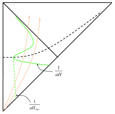
Figure 1: The causal patch diagram of slow expansion scenario. The universe is initially in Minkowski space, which then slowly expands, reheats and evolves with big-bang cosmology. The black dashed line is the reheating surface. The orange lines are the comoving perturbation modes, which leave its comoving horizon $1/(aH_{Per})$, but their wavelengths remain smaller than $1/(aH)$.

The slow expansion is the evolution with $\epsilon=-{\dot{H}}/H^{2}\ll-1$. We may write it as [11]

$$a\sim(-t)^{-p},$$ (3)

in which $0<p=1/|\epsilon|\ll 1$ is constant, which is the scale solution, or [12][32]

$$a\sim e^{{1\over(-t)^{n}}}\simeq 1+{1\over(-t)^{n}},$$ (4)

in which $n>0$ and $\epsilon\sim-(-t)^{n}$, which is the Minkowski spacetime in infinite past, and when ${1/(-t)^{n}}\sim 1$, the slow expansion ends. It has been observed earlier in [11] that such a spacetime might be responsible for scale-invariant adiabatical perturbation, and after the end of the slowly expanding phase, the universe may reheat and start to evolve with standard cosmology. However, how to remove the ghost instability still remains a challenging issue. Recently, we have implemented the corresponding scenarios ghost-freely in [12] for (4) with $n=4$, and in [13] for (3).

The physics of the origin of primordial perturbations is illustrated as follows, see also the causal patch diagram in Fig.1. The perturbation mode with wavelength $a\lambda\gg 1/H_{Per}$ will freeze and become the primordial perturbation, otherwise it will oscillate inside $1/H_{Per}$. Here, $1/H_{Per}$ is the sound horizon of the perturbations, see Eq.(24) and (35) for its explicit expression. During inflation, $1/(aH_{Per})$ nearly coincide with $1/(aH)$, which suggests that the shape of perturbation spectrum is mainly set up by the background evolution. However, during slow expansion, $1/(aH_{Per})\ll 1/(aH)$, so the background is irrelevant with the origin of primordial perturbation, as clarified recently also by Wetterich in [31].

In (4), the physical meaning of $n$ is the “slow-degree” of expansion. The larger is $n$, the slower is the corresponding expansion. It should be mentioned that $n=2$ is that of the Galilean genesis [33][34], so the background (4) is also called the generalized genesis in [35], in which it was clarified that the scale-invariant adiabatic perturbation can appear only for $n=4$. When $n\ll 1$, (4) actually reduces to (3) with $p=n$, since

$$H={n\over(-t)^{1+n}}\simeq{p\over(-t)}$$ (5)

for $n\ll 1$. When $n\gg 1$, the expansion is the slowest, (4) may be replaced with

$$a\sim e^{1/(e^{-t})}\simeq 1+1/(e^{-t}),$$ (6)

noting that initially $t\ll-1$, which runs towards $t\simeq 0$. How the scale-invariant adiabatical perturbation emerges from (6) was discussed in [36]. The background (6) actually equals to that in emergent scenario [37], however, in which it was implemented by introducing a positive curvature, so its initial state is not flat Minkowski space, see also [38].

As has been commented, the primordial GWs produced is generally strong blue-tilt, which is negligible on large scale. However, if $M_{P,eff}^{2}\sim{1\over(t_{*}-t)^{2}}$ is rapidly increasing during slow expansion, which may be induced by the nonminimal coupling of the scalar field to gravity, the primordial GWs may be scale-invariant [13].

III The model with nonminimal derivative coupling

III.1 The Langrangian

Here, we begin with

$$S=\int dtd^{3}x\sqrt{-g}\left({\cal L}_{1}+{\cal L}_{2}\right)+{S}_{matter},$$ (7)

and

$${\cal L}_{1}=-\,e^{4\phi/{\cal M}}X+{1\over{\cal M}^{8}}X^{3}-\alpha{\cal M}^{4}\,e^{6\phi/{\cal M}},$$ (8)

$${\cal L}_{2}={M_{P}^{2}\over 2}\left({\cal M}^{8}/X^{2}+1\right)R+{M_{P}^{2}{\cal M}^{8}\over X^{3}}\left[-\left(\Box\phi\right)^{2}+\nabla_{\mu}\nabla_{\nu}\phi\nabla^{\mu}\nabla^{\nu}\phi\right],$$ (9)

where $X=-{\nabla_{\mu}\phi\nabla^{\mu}\phi/2}$ and $\Box\phi=g^{\mu\nu}\nabla_{\mu}\nabla_{\nu}\phi$, ${S}_{matter}$ is that of all components minimally coupling to the metric, and ${\cal M}\ll M_{P}$, and $\alpha$ is constant. Our (7) is actually a subclass of Horndeski theory [39], which suggests that the equation of motion is not higher than second order. The nonminimally derivative coupling may be also $G_{\mu\nu}\partial^{\mu}\phi\partial^{\nu}\phi$, which is also interesting [40][41][42][43][44][45][46][47][48].

III.2 The background of slow-expansion

Below we will derive the equation of motion for (7), and obtain the slowly expanding solution. The calculation is slightly similar to that in [12].

The Friedmann equation is

$$3M_{P}^{2}H^{2}\left(1-\frac{15{\cal M}^{8}}{X^{2}}\right) = \rho_{eff}$$ (10)

$$= -\,e^{4\phi/{\cal{\cal M}}}X+{5\over{\cal{\cal M}}^{8}}X^{3}+\alpha{\cal M}^{4}\,e^{6\phi/{\cal M}}.$$

Here, $\rho_{tot}=3M_{P}^{2}H^{2}=\rho_{eff}+45M_{P}^{2}H^{2}{\cal M}^{8}/X^{2}>0$, and $\rho_{eff}$ is that without the contribution from the derivative coupling to gravity. We focus on the slowly expanding solution, i.e., $H\simeq 0$ [11], which requires $\rho_{eff}\simeq 0$. In addition, we also require $\rho_{eff,X}=0$ to avoid the divergence of the scalar spectrum, see Sec. IV.2 for details. Both these two conditions fix the evolution of $\phi$ as

$$e^{\phi/{\cal M}}=\left({15\over 4}\right)^{1/4}{1\over{\cal M}(t_{*}-t)},$$ (11)

$${\dot{\phi}}={{\cal M}\over(t_{*}-t)},$$ (12)

and $\alpha={2\over 3\sqrt{15}}$, where initially $t$ is in negative infinity and runs towards $t_{*}$. Thus only one adjustable parameter ${\cal M}$ in (7) is left, which, we will see, determines the amplitude of primordial GWs.

Figure 2: The evolutions of the background, $1/H$, $1/H_{T}$ and $1/H_{\cal R}$. There is a brief reheating era between the end of the slow expansion era and the beginning of the radiation dominated era.

Using $\rho_{eff}\simeq 0$, the evolution of $\dot{H}$ is given as

$$10{{\cal M}^{8}M_{P}^{2}\over X^{2}}{\dot{H}} \simeq e^{4\phi/{\cal{\cal M}}}X-{1\over{\cal{\cal M}}^{8}}X^{3}+\alpha{\cal M}^{4}\,e^{6\phi/{\cal M}}+20{{\cal M}^{8}M_{P}^{2}\over X^{3}}H{\dot{\phi}}{\ddot{\phi}}$$ (13)

$$= {24\over{\cal{\cal M}}^{8}}X^{3}+20{{\cal M}^{8}M_{P}^{2}\over X^{3}}H{\dot{\phi}}{\ddot{\phi}}.$$

After combining Eq.(12), we have

$${\dot{H}}\sim{1\over{\cal M}^{6}M_{P}^{2}}(t_{*}-t)^{-10},$$ (14)

which straightly gives

$$H\sim{1\over{\cal M}^{6}M_{P}^{2}}(t_{*}-t)^{-9}.$$ (15)

The growing of $H$ suggests the violation of the null energy condition. However, the model is free of ghost instability, as will be showed in Sec.IV. The evolution of cosmological background is

$$a=a_{0}e^{\int Hdt}\simeq a_{0}(1+{1\over{\cal M}^{6}M_{P}^{2}}{1\over(t_{*}-t)^{8}})\simeq a_{0}.$$ (16)

Thus initially the universe is nearly Minkowski. Here, (16) corresponds to (4) with $n=8$. We plot the evolution sketch of the background and $1/H$ in Fig.2.

We see from (16) that the condition of slow expansion is

$${\cal M}^{6}M_{P}^{2}(t_{*}-t)^{8}\gg 1,$$ (17)

which means $\epsilon\simeq-{\cal M}^{6}M_{P}^{2}(t_{*}-t)^{8}\ll-1$. When the condition (17) is broken, the slowly expanding phase ends, and ${\cal M}^{6}M_{P}^{2}(t_{*}-t)^{8}\simeq 1$ signals the ending time $t_{e}$

$$t_{*}-t_{e}\simeq{1\over M_{P}^{1/4}{\cal M}^{3/4}}.$$ (18)

Hereafter, ${X/{\cal M}^{4}}\gg 1$, so GR is recovered in (7), the universe will evolve with the standard cosmology.

IV The power spectrum of primordial perturbations

IV.1 The primordial GWs

We will calculate the primordial perturbations from nearly Minkowski background (16). Tensor mode $\gamma_{ij}$ satisfies $\gamma_{ii}=0$, and $\partial_{i}\gamma_{ij}=0$, and its quadratic action for (7) is

$$S^{(2)}=\int d\tau d^{3}x\,{a^{2}Q_{T}\over 8}\left[\gamma_{ij}^{\prime 2}-c_{T}^{2}(\vec{\nabla}\gamma_{ij})^{2}\right],$$ (19)

where

$$Q_{T}=M_{P}^{2}\left(1+{5{\cal M}^{8}\over X^{2}}\right)\simeq 20M_{P}^{2}{\cal M}^{4}(t_{*}-t)^{4},$$ (20)

and

$$c_{T}=\sqrt{\frac{1+{\cal M}^{8}/X^{2}}{1+5{\cal M}^{8}/X^{2}}}\simeq\sqrt{1/5}$$ (21)

is the propagation speed of GWs. See Appendix A for a notebook. Because $Q_{T}>0$ and $c_{T}^{2}>0$, there is no ghost instability.

In the momentum space,

$$\gamma_{ij}(\tau,\mathbf{x})=\int\frac{d^{3}k}{(2\pi)^{3}}e^{-i\mathbf{k}\cdot\mathbf{x}}\sum_{\lambda=+,\times}\hat{\gamma}_{\lambda}(\tau,\mathbf{k})\epsilon^{(\lambda)}_{ij}(\mathbf{k}),$$ (22)

where $\hat{\gamma}_{\lambda}(\tau,\mathbf{k})=\gamma_{\lambda}(\tau,k)a_{\lambda}(\mathbf{k})+\gamma_{\lambda}^{*}(\tau,-k)a_{\lambda}^{{\dagger}}(-\mathbf{k})$, the polarization tensors $\epsilon_{ij}^{(\lambda)}(\mathbf{k})$ satisfy $k_{j}\epsilon_{ij}^{(\lambda)}(\mathbf{k})=0$ and $\epsilon_{ii}^{(\lambda)}(\mathbf{k})=0$, and $\epsilon_{ij}^{(\lambda)}(\mathbf{k})\epsilon_{ij}^{*(\lambda^{\prime})}(\mathbf{k})=\delta_{\lambda\lambda^{\prime}}$, $\epsilon_{ij}^{*(\lambda)}(\mathbf{k})=\epsilon_{ij}^{(\lambda)}(-\mathbf{k})$, the commutation relation for the annihilation and creation operators $a_{\lambda}(\mathbf{k})$ and $a^{{\dagger}}_{\lambda}(\mathbf{k}^{\prime})$ is $[a_{\lambda}(\mathbf{k}),a_{\lambda^{\prime}}^{{\dagger}}(\mathbf{k}^{\prime})]=\delta_{\lambda\lambda^{\prime}}\delta^{(3)}(\mathbf{k}-\mathbf{k}^{\prime})$.

The equation of motion for $h_{\lambda}(\tau,k)$ is

$$u^{\prime\prime}+\left(c_{T}^{2}k^{2}-\frac{z_{T}^{\prime\prime}}{z_{T}}\right)u=0,$$ (23)

where $\gamma_{\lambda}(\tau,k)={u}(\tau,k)/{z_{T}}$ and $z_{T}=a{\sqrt{Q_{T}}}/2$. Initially, the perturbations are deep inside its own horizon $c_{T}/H_{T}$, which means $c_{T}^{2}k^{2}\gg\frac{z_{T}^{\prime\prime}}{z_{T}}$. The GWs horizon $\sim 1/H_{T}$ is defined as

$$H_{T}={1\over a}\sqrt{\frac{z_{T}^{\prime\prime}}{z_{T}}}\sim{1\over t_{*}-t}.$$ (24)

Here, since ${1/H\over c_{T}/H_{T}}\sim{\cal M}^{6}M_{P}^{2}(t_{*}-t)^{8}\gg 1$, even if the perturbations leave their own horizon $c_{T}/H_{T}$, they remain inside $1/H$, see Fig.2. The primordial GWs spectrum is determined by $z_{T}=a\sqrt{Q_{T}}$. Due to the rapid evolution of $Q_{T}$, the evolution of background is now irrelevant to the origin of primordial perturbation. The initial state of perturbation is the Minkowski vacuum,

$$u\sim\frac{1}{\sqrt{2c_{T}k}}e^{-ic_{T}k\tau}.$$ (25)

When $c_{T}^{2}k^{2}\ll\frac{z_{T}^{\prime\prime}}{z_{T}}$, i.e. the wavelength of perturbation is far larger than its horizon $c_{T}/H_{T}$, the solution of Eq.(23) is given by

$$u/z_{T}\sim C+\int D{d\tau\over a^{2}Q_{T}},$$ (26)

where $C$ is the constant mode, while $D$ is the growing mode, $D\int{d\tau\over a^{2}Q_{T}}\sim{1\over(t_{*}-t)^{3}}$, which will dominate the perturbation. We have

$$|u|\simeq{1\over\sqrt{2c_{T}k}}\left(c_{T}k\tau_{*}-c_{T}k\tau\right)^{-1}.$$ (27)

The power spectrum of primordial GWs is

$${\cal P}_{T}^{1/2}={k^{3/2}\over\sqrt{2\pi^{2}}}\sqrt{\sum_{\lambda=+,\times}|\gamma_{\lambda}|^{2}}=\sqrt{4k^{3}\over\pi^{2}}{|u|\over a\sqrt{Q_{T}}}.$$ (28)

Since the growing model dominates the perturbation, the amplitude of perturbation will increase until the slow-expansion phase ends, e.g.[12]. Therefore, the resulting spectrum of ${\cal P}_{T}$ should be calculated at $t_{e}$. Thus with Eq.(18) and (27), we have

$${\cal P}_{T}^{1/2}\simeq\sqrt{1\over 10\pi^{2}}{1\over c_{T}^{3/2}M_{P}{\cal M}^{2}(t_{*}-t_{e})^{3}}\simeq\sqrt{5^{1/2}\over 2\pi^{2}}\left({{\cal M}\over M_{P}}\right)^{1/4}.$$ (29)

This indicates that the primordial GWs is scale-invariant with the amplitude $({\cal M}/M_{P})^{1/4}$, and the only adjustable parameter $\cal M$ may be fixed by the observation.

IV.2 The primordial scalar perturbations

The quadratic action for the curvature perturbation $\cal R$ is

$$S^{(2)}_{\cal R}=\int d\tau d^{3}x\,{a^{4}Q_{\cal R}}\left[{\dot{\cal R}}^{2}-{c_{\cal R}^{2}\over a^{2}}(\vec{\nabla}{\cal R})^{2}\right],$$ (30)

where

$$Q_{\cal R}\simeq 10{{\cal M}^{8}M_{P}^{2}\over X^{2}}\sim M_{P}^{2}{\cal M}^{4}(t_{*}-t)^{4},$$ (31)

$$c_{\cal R}^{2}\sim M_{P}^{2}{\cal M}^{6}(t_{*}-t)^{8},$$ (32)

see Appendix A for a notebook. It should be mentioned that if $\rho_{eff,X}\neq 0$, we will have $Q_{\cal R}\sim(t_{*}-t)^{12}$ and $c_{\cal R}^{2}$ is constant, so that the spectrum of $\cal R$ will be strongly red, which will make the amplitude of $\cal R$ diverge on the largest scale.

Here, the sound speed changes rapidly. It is convenient to redefine the conformal ‘time’ as $dy=c_{\cal R}d\tau$ or $d\tilde{y}=c_{\cal R}dt$, e.g.[49], which implies

$$\tilde{y}_{*}-\tilde{y}\sim{M_{P}{\cal M}^{3}\over 5}(t_{*}-t)^{5}.$$ (33)

Thus the equation of motion for $\cal R$ is

$$\frac{d^{2}v_{\cal R}}{dy^{2}}+\left(k^{2}-\frac{d^{2}z_{\cal R}/dy^{2}}{z_{\cal R}}\right)v_{\cal R}=0,$$ (34)

where ${\cal R}={v}_{\cal R}(\tau,k)/{z_{\cal R}}$ and $z_{\cal R}=a{\sqrt{c_{\cal R}Q_{\cal R}}}$.

Initially, the perturbations are deep inside its own horizon $1/H_{\cal R}$, which means $k^{2}\gg\frac{d^{2}z_{\cal R}/dy^{2}}{z_{\cal R}}$. We have

$${H}_{\cal R}={1\over a}\sqrt{\frac{d^{2}z_{\cal R}/dy^{2}}{z_{\cal R}}}\sim{1\over y_{*}-y}\sim{1\over(t_{*}-t)^{5}}.$$ (35)

Thus we see $1/H_{T}\ll 1/H_{\cal R}\ll 1/H$, see Fig.2. Since the evolution of ${H}_{T}$ is distinguished from that of ${H}_{\cal R}$, the tilt of the $\cal R$ spectrum must be different from that of GWs.

The initial state of perturbation is the Minkowski vacuum,

$$v_{\cal R}\sim\frac{1}{\sqrt{2k}}e^{-iky}.$$ (36)

When $k^{2}\ll\frac{d^{2}z_{\cal R}/dy^{2}}{z_{\cal R}}$, the solution of Eq.(34) is

$$|v_{\cal R}|\simeq{1\over\sqrt{2k}}\left(ky_{*}-ky\right)^{1/5},$$ (37)

noting that $z_{\cal R}\sim aM_{P}^{7/10}{\cal M}^{11/10}(\tilde{y}_{*}-\tilde{y})^{4/5}$. Thus the power spectrum of $\cal R$ is

$${\cal P}_{\cal R}^{1/2} = {k^{3/2}\over\sqrt{2\pi^{2}}}\left|v_{\cal R}\over z_{\cal R}\right|\simeq{1\over M_{P}^{5/2}{\cal M}^{13/2}(t_{*}-t)^{9}}\left(ky_{*}-ky_{e}\right)^{6/5}$$ (38)

$$\simeq \left({{\cal M}\over M_{P}}\right)^{1/4}\left(ky_{*}-ky_{e}\right)^{6/5}.$$

Thus the spectral index is $n_{\cal R}-1=12/5$. Here, similar to GWs, the growing mode dominates the perturbation, so the resulting spectrum of ${\cal P}_{T}$ should be calculated at $t_{e}$.

The amplitude of $\cal R$ spectrum should be same with that of GWs, but since $n_{\cal R}-1=12/5$, the spectrum is blue-tilt, on large scale the amplitude of $\cal R$ is negligible. This can be shown as follows. We have $y_{*}-y_{e}\simeq 1/(aM_{P}^{1/4}{\cal M}^{3/4})$ in light of Eq.(33), which just equals to $1/k_{e}=1/(aH_{e})$. The efolds number for the primordial perturbations is defined as ${\cal N}=\ln(k/k_{e})$. Thus ${\cal P}_{\cal R}$ may be rewritten as

$${\cal P}_{\cal R}\simeq\left({{\cal M}\over M_{P}}\right)^{1/2}e^{{12{\cal N}\over 5}},$$ (39)

where ${\cal N}<0$ since $k<k_{e}$. For ${\cal N}>0$, the corresponding perturbation modes exits horizon after $t_{e}$, thus will experience the evolution other than the slow expansion. We assume ${\cal P}_{T}\sim 10^{-11}$, and plot ${\cal P}_{T}$ and ${\cal P}_{\cal R}$ in Eqs.(29) and (39) with respect to $\cal N$, respectively, in Fig.3. We can see that on far smaller scale, the amplitude of scalar perturbation is same with that of GWs, but on large scales, ${\cal P}_{\cal R}$ is negligible. Here, it is obvious that the adiabatic perturbation is not able to be responsible for the CMB fluctuation and large scale structure.

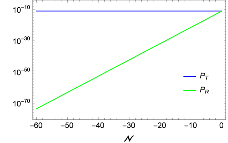
Figure 3: ${\cal P}_{T}$ and ${\cal P}_{\cal R}$ with respect to the efolds number ${\cal N}=\ln(k/k_{e})$.

However, the curvature perturbation may also be induced by the entropy perturbation from a light scalar field $\chi$ with

$${\cal L}_{\chi}\sim-{1\over 2}e^{-{2\lambda\over\cal M}\phi}(\partial\chi)^{2},$$ (40)

or nonminimally coupling to the gravity ${\cal L}_{\chi}\sim-e^{-{2\lambda\over\cal M}\phi}G_{\mu\nu}\partial^{\mu}\chi\partial^{\nu}\chi$ [41][50], where $\lambda$ is the dimensionless constant. Defining $u_{\chi}=z_{\chi}\delta\chi$ and $z_{\chi}\sim ae^{-{\lambda\over\cal M}\phi}$, for (40), we have the perturbation equation of $\delta\chi$ as

$$u_{\chi}^{\prime\prime}+\left(k^{2}-\frac{z_{\chi}^{\prime\prime}}{z_{\chi}}\right)u_{\chi}=0,$$ (41)

where

$$\frac{z_{\chi}^{\prime\prime}}{z_{\chi}}\simeq\frac{\lambda^{2}-\lambda}{(\tau_{*}-\tau)^{2}}.$$ (42)

The power spectrum of $\delta\chi$ is ${\cal P}_{\delta\chi}={k^{3}\over 2\pi^{2}}|\delta\chi|^{2}$. Here, the mechanism is similar to that applied to the ekpyrotic model, see Refs. [20][21][22][51][52] for the details, which may result in a local non-Gaussianity with $f_{NL}\sim{\cal O}(1)$. When $\lambda=2$ or $-1$, ${\cal P}_{\delta\chi}$ will be scale-invariant, see also [53]. Then, we obtain

$$u_{\chi}\simeq-{i\over\sqrt{2k}}\cdot{1\over k(\tau_{*}-\tau)}\,,$$ (43)

for $k(\tau_{*}-\tau)\ll 1$. Thus

$$|\delta\chi|={1\over\sqrt{2k^{3}}}\left({15\over 4}\right)^{\lambda/4}\left(M_{p}\over{\cal M}\right)^{\lambda+1\over 4}{\cal M}\,.$$ (44)

After the slowly expanding phase ends, the universe reheats, $\delta\chi$ may be convert to the curvature perturbation. We follow Ref. [54], and assume that during reheating, the background field $\phi$ couples to ordinary particles as $g^{2}\,\phi\,q\,q$, where $q$ represents the ordinary particles, and $g$ is the coupling strength. Thus the decay rate of $\phi$ is $\Gamma\sim g^{2}$. The coupling strength can be $\chi$-dependent,

$$g=g_{0}\left(1+{\chi\over{\cal M}_{\star}}\right),$$ (45)

where ${\cal M}_{\star}$ is the scale with mass dimension. After reheating, $\rho\sim T^{4}_{reh}$, and the reheating temperature $T_{reh}\sim\sqrt{\Gamma}\sim g$. We have

$${\cal R}={\delta\rho\over\rho}={4\delta\chi\over{\cal M}_{\star}}\,,$$ (46)

noting ${\delta T_{reh}/T_{reh}}={\delta g/g}={\delta\chi/{\cal M}_{\star}}$.

When $\lambda=-1$, we have

$$|\delta\chi|={1\over\sqrt{k^{3}}}\left({1\over 15}\right)^{1/4}{\cal M}\,.$$ (47)

Then the power spectrum of $\cal R$ induced by $\delta\chi$ is

$${\cal P}^{\delta\chi}_{\cal R}={k^{3}\over 2\pi^{2}}|{\cal R}|^{2}={8\over\sqrt{15}\pi^{2}}\left({{\cal M}\over{\cal M}_{\star}}\right)^{2}\,.$$ (48)

Thus with (29), we have

$$r={{\cal P}_{T}\over{\cal P}^{\delta\chi}_{\cal R}}={5\sqrt{3}{\cal M}_{\star}^{2}\over 16\sqrt{{\cal M}^{3}M_{P}}}\,.$$ (49)

Recent observations suggested $r<0.1$ [5], which puts the bound ${\cal M}_{\star}<0.43M_{P}^{1/4}{\cal M}^{3/4}$. Moreover, by requiring $\lambda$ to slightly deviate from $-1$, we will obtain a nearly scale-invariant scalar spectrum with slight red tilt.

IV.3 The Minkowski space with asymptotic-past free gravity

As was showed in Sec.III.2, the initial universe is in a flat Minkowski space. The initial background is not spoiled by the perturbations, since the average square of the amplitude of $\cal R$ in infinite past is

$$<{\cal R}^{2}>={1\over 8\pi^{3}}\int^{aH}_{aH/e}|{\cal R}|^{2}d^{3}k\simeq{H^{12/5}\over{\cal M}^{11/10}M_{P}^{13/10}}\longrightarrow 0.$$ (50)

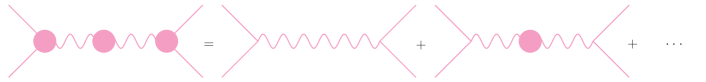
Figure 4: One particle reducible graphs for the gravity interaction, in which the solid circles denote the full set of radiation corrections to the vertex function and the graviton propagator.

In initial Minkowski space with $a=a_{0}$, see (16), the cubic action of tensor perturbation [55] and, e.g., the interaction between it and the Dirac field [56], are

$$S^{(3)}=\int d^{4}x{a_{0}c_{T}^{2}Q_{T}\over 4}\left(\gamma_{ik}\gamma_{jl}-{\gamma_{ij}\gamma_{kl}\over 2}\right)\partial_{k}\partial_{l}\gamma_{ij},$$ (51)

$${S}_{\psi{\bar{\psi}}\gamma}^{(3)} = \int d^{4}x{a^{2}_{0}\over 2}T^{ij}\gamma_{ij}$$ (52)

$$= i\int d^{4}x~{}\frac{a_{0}^{2}}{8}\left(\bar{\psi}\gamma^{i}(\partial^{j}\psi)+\bar{\psi}\gamma^{j}(\partial^{i}\psi)-(\partial^{i}\bar{\psi})\gamma^{j}\psi-(\partial^{j}\bar{\psi})\gamma^{i}\psi\right)\gamma_{ij},$$

respectively. We redefine $\gamma_{ij}$ as $M_{P,eff}\gamma_{ij}/2$ [57], and write (51) and (52) as

$$S^{(3)}=\int a_{0}d^{4}x{2\over M_{P,eff}}\left(\gamma_{ik}\gamma_{jl}-{\gamma_{ij}\gamma_{kl}\over 2}\right)\partial_{k}\partial_{l}\gamma_{ij},$$ (53)

$${S}_{\psi{\bar{\psi}}\gamma}^{(3)} = \int a_{0}^{2}d^{4}x{1\over M_{P,eff}}T^{ij}\gamma_{ij},$$ (54)

where $M_{P,eff}=c_{T}\sqrt{Q_{T}}$. The strength of the gravitational interaction is determined by a set of one particle reducible graphs, see Fig.4. Thus, after neglecting the tensor index, we may write the renormalizated effective Newton constant $G_{N,ren}$ as

$$i{G_{N,ren}\over p^{2}}={i\over M_{P,eff}^{2}p^{2}}+{i\over M_{P,eff}^{2}p^{2}}(loop){i\over M_{P,eff}^{2}p^{2}}+\cdots.$$ (55)

Initially, $M_{P,eff}=\sqrt{c_{T}^{2}Q_{T}}\sim(t_{*}-t)^{2}$ is infinite large, which implies $G_{N,ren}=0$. Thus from $t<t_{e}$, if we back to the infinite past, the gravitational force will fade gradually and disappear eventually. This suggests that the gravity is asymptotic-past free.

However, after $t\simeq t_{e}$,

$${X\over{\cal M}^{4}}\simeq{1\over{\cal M}^{2}(t_{*}-t_{e})^{2}}=\left({M_{P}\over{\cal M}}\right)^{1/2}\gg 1$$ (56)

we will have $M_{P,eff}\simeq M_{P}$, GR is recovered, hereafter the universe will evolve with the standard cosmology. Thus the asymptotic-past freedom of gravity is not conflicted with our current observations.

V See it in Einstein frame

V.1 The Langrangian

In principle, for the action with nonminimal coupling to gravity, it is always possible to rewrite it to the Einstein-Hilbert’s, in which the Ricci scalar is minimally coupled.

We rescale the metric as

$$g_{\mu\nu}={\cal A}^{2}({\hat{X}})\hat{g}_{\mu\nu},$$ (57)

which implies

$$g=\hat{g}{\cal A}^{8},\qquad R=\frac{\hat{R}}{{\cal A}^{2}}-\frac{6{\hat{\nabla}}_{\mu}{\hat{\nabla}}^{\mu}{\cal A}}{{\cal A}^{3}},$$ (58)

$$\Box\phi=\frac{\hat{\Box}\phi}{{\cal A}^{2}}+\frac{2{\hat{\nabla}}_{\mu}{\cal A}{\hat{\nabla}}^{\mu}\phi}{{\cal A}^{3}},\qquad X=\frac{\hat{X}}{{\cal A}^{2}}.$$ (59)

Thus for (7), we have

$$S=\frac{M_{p}^{2}}{2}\int d^{4}x\sqrt{-{\hat{g}}}{\cal A}^{2}(1+\frac{{\cal M}^{8}}{{\hat{X}}^{2}}{\cal A}^{4}){\hat{R}}+\cdots,$$ (60)

which is Einstein-Hilbert style requires ${\cal A}^{2}(1+\frac{{\cal M}^{8}}{{\hat{X}}^{2}}{\cal A}^{4})=1$. This gives

$${\cal A}=\frac{{\hat{X}}^{1/3}}{{\cal M}^{4/3}}={X\over{\cal M}^{4}},$$ (61)

since $\frac{{\cal M}^{8}}{{\hat{X}}^{2}}{\cal A}^{4}\gg 1$ during the slow expansion. The line element is $d\hat{s}^{2}={\cal A}^{-2}ds^{2}=\hat{g}_{\mu\nu}dx^{\mu}dx^{\nu}$. It’s convenient to redefine $d{\tilde{t}}={\cal A}^{-1}dt$ and $\tilde{a}={\cal A}^{-1}a$, which make us back to the Einstein frame $d\tilde{s}^{2}=d\hat{s}^{2}=\tilde{g}_{\mu\nu}d\tilde{x}^{\mu}d\tilde{x}^{\nu}=-d\tilde{t}^{2}+\tilde{a}^{2}d\mathbf{x}^{2}$, in which (60) becomes

$$S_{E} = \frac{M_{P}^{2}}{2}\int d\tilde{t}d^{3}\mathbf{x}\sqrt{-\tilde{g}}\Big{(}{\tilde{R}}-2\alpha\frac{{\tilde{X}}^{4/3}}{M_{P}^{2}{\cal M}^{4/3}}e^{6\phi/{\cal M}}-2\frac{{\tilde{X}}^{5/3}}{M_{P}^{2}{\cal M}^{8/3}}e^{4\phi/{\cal M}}$$ (62)

$$+2\frac{{\tilde{X}}^{7/3}}{M_{P}^{2}{\cal M}^{16/3}}-2\frac{({\tilde{\nabla}}_{\mu}{\tilde{\nabla}}^{\mu}\phi)^{2}}{\tilde{X}}-\frac{4}{9}\frac{({\tilde{\nabla}}_{\mu}{\tilde{X}}{\tilde{\nabla}}^{\mu}\phi)^{2}}{{\tilde{X}}^{3}}-2\frac{{\tilde{\nabla}}_{\mu}{\tilde{\nabla}}^{\mu}{\tilde{X}}}{{\tilde{X}}}$$

$$-2\frac{{\tilde{\nabla}}_{\mu}{\tilde{\nabla}}^{\mu}{\tilde{X}}}{{\cal M}^{8/3}{\tilde{X}}^{1/3}}+\frac{4}{9}\frac{{\tilde{\nabla}}_{\mu}{\tilde{X}}{\tilde{\nabla}}^{\mu}{\tilde{X}}}{{\tilde{X}}^{2}}+\frac{4}{3}\frac{{\tilde{\nabla}}_{\mu}{\tilde{X}}{\tilde{\nabla}}^{\mu}{\tilde{X}}}{{\cal M}^{8/3}{\tilde{X}}^{4/3}}-\frac{4}{3}\frac{{\tilde{\nabla}}_{\mu}\phi{\tilde{\nabla}}^{\mu}{\tilde{X}}{\tilde{\nabla}}_{\nu}{\tilde{\nabla}}^{\nu}\phi}{{\tilde{X}}^{2}}$$

$$-\frac{8}{3}\frac{{\tilde{\nabla}}^{\mu}{\tilde{X}}{\tilde{\nabla}}^{\nu}\phi{\tilde{\nabla}}_{\nu}{\tilde{\nabla}}_{\mu}\phi}{{\tilde{X}}^{2}}+2\frac{{\tilde{\nabla}}_{\mu}{\tilde{\nabla}}_{\nu}\phi{\tilde{\nabla}}^{\mu}{\tilde{\nabla}}^{\nu}\phi}{\tilde{X}}\Big{)}.$$

V.2 The background

The evolutions of ${\tilde{H}}={d{\tilde{a}}\over d\tilde{t}}/{\tilde{a}}$ and $\dot{\tilde{H}}$ are

$$3{\tilde{H}}^{2}M_{P}^{2} = -\alpha e^{6\phi/{\cal M}}\frac{{\tilde{X}}^{4/3}}{15{\cal M}^{4/3}}+e^{4\phi/{\cal M}}\frac{{\tilde{X}}^{5/3}}{15{\cal M}^{8/3}}-\frac{{\tilde{X}}^{7/3}}{3{\cal M}^{16/3}}$$ (63)

$$-2M_{P}^{2}\frac{{\tilde{H}}\dot{\phi}\ddot{\phi}}{\tilde{X}}-4M_{P}^{2}\frac{{\tilde{H}}\dot{\phi}\ddot{\phi}}{5{\cal M}^{8/3}{\tilde{X}}^{1/3}}-2M_{P}^{2}\frac{\ddot{\phi}^{2}}{3\tilde{X}}$$

$$-2M_{P}^{2}\frac{\ddot{\phi}^{2}}{45{\cal M}^{8/3}{\tilde{X}}^{1/3}}-4M_{P}^{2}\frac{\dot{\phi}\dddot{\phi}}{15{\cal M}^{8/3}{\tilde{X}}^{1/3}}\,\,,$$

$$\dot{\tilde{H}} = e^{6\phi/{\cal M}}\frac{2\alpha{\tilde{X}}^{4/3}}{15{\cal M}^{4/3}M_{P}^{2}}+e^{4\phi/{\cal M}}\frac{{\tilde{X}}^{5/3}}{15{\cal M}^{8/3}M_{P}^{2}}+\frac{{\tilde{X}}^{7/3}}{15{\cal M}^{16/3}M_{P}^{2}}$$ (64)

$$+\frac{{\tilde{H}}\dot{\phi}\ddot{\phi}}{\tilde{X}}+\frac{2{\tilde{H}}\dot{\phi}\ddot{\phi}}{5{\cal M}^{8/3}{\tilde{X}}^{1/3}}+\frac{\ddot{\phi}^{2}}{\tilde{X}}+\frac{4\ddot{\phi}^{2}}{45{\cal M}^{8/3}{\tilde{X}}^{1/3}}-\frac{\dot{\phi}\dddot{\phi}}{3\tilde{X}}+\frac{2\dot{\phi}\dddot{\phi}}{15{\cal M}^{8/3}{\tilde{X}}^{1/3}}\,\,,$$

respectively. Note that only in this subsection a dot denotes $d/d\tilde{t}$. Here, both equations involve the higher-order derivatives of $\phi$. Thus straightly acquiring the solution of background is difficult. However, it is convenient to calculate it by using the conformal relation (61). We have

$${\cal A}={X\over{\cal M}^{4}}={1\over{2}{\cal M}^{2}(t_{*}-t)^{2}},$$ (65)

where Eq.(12) is applied. Then noticing $d{\tilde{t}}={\cal A}^{-1}dt$, we have ${\tilde{t}}_{*}-{\tilde{t}}=2{\cal M}^{2}(t_{*}-t)^{3}/3$. Thus the background is

$$\tilde{a}(\tilde{t})={\cal A}^{-1}a_{0}(1+{1\over{\cal M}^{6}M_{P}^{2}}{1\over(t_{*}-t)^{8}})\simeq a_{0}{\cal M}^{2/3}({\tilde{t}_{*}}-{\tilde{t}})^{2/3},$$ (66)

which is the matter contraction [58][59], also [8].

V.3 The physical background

The frame that the matter minimally couples to the metric may be called the matter frame. The conformally dual models can be distinguished when we see from the matter point of view, as has been clarified in [60], or by applying the Weyl-invariants [28]

$$\Theta_{m}=\left(H+\frac{\dot{m}}{m}\right)M_{P,eff}^{-1},$$ (67)

$$\Theta_{P}=\left(H+\frac{\dot{M}_{P,eff}}{M_{P,eff}}\right)M_{P,eff}^{-1}$$ (68)

where $\Theta_{m}$ defines a physical ruler measuring the evolution of background, the physical ruler is comprised of particles with mass $m$, $S_{matter}=\int mds$, and its length scale is set by the Compton wavelength $\lambda_{Compton}\sim 1/m$ of the particle, $\Theta_{m}>0$ signals that the background felt by the matter is expanding, otherwise it is contracting, while $\Theta_{P}=({{\dot{z}_{T}}/z_{T}})M_{P,eff}^{-1}$ measures the evolutive behavior of $1/H_{T}$, and so the primordial GWs, the conformal invariance of perturbations suggests that conformally dual models have same $\Theta_{P}$. The inflation corresponds to $\Theta_{m}>0$, $\Theta_{P}>0$, while the ekpyrosis is $\Theta_{m}<0$, $\Theta_{P}<0$. Recently, the anamorphic universe proposed in [28] corresponds to $\Theta_{m}<0$, $\Theta_{P}>0$.

We focus on the slow expansion model proposed here. We have $\dot{m}=0$, since the matter minimally couples to the metric, and the effective Planck mass

$$M_{P,eff}=\sqrt{c_{T}^{2}Q_{T}}=M_{P}\sqrt{1+\frac{{\cal M}^{8}}{X^{2}}}\sim(t_{*}-t)^{2}.$$ (69)

Thus $\Theta_{m}\sim H>0$ and $\Theta_{P}\sim\frac{\dot{M}_{P,eff}}{M_{P,eff}}<0$, see also [30] for conflation. $\Theta_{m}>0$ suggests our cosmological background is actually a physical expansion when measured relative to a physical ruler ${\tilde{\lambda}}_{Compton}$, regardless of the frames. Actually, it’s easy to check that in Einstein frame, ${\tilde{\lambda}}_{Compton}\sim 1/\tilde{m}\sim(\tilde{t}_{*}-\tilde{t})^{2/3}$ is actually contracted slightly faster than $\tilde{a}$, in which $S_{matter}=\int\tilde{m}d{\tilde{s}}$ and $\tilde{m}=m\cal A$. Thus the universe is a physical expansion when compared with ${\tilde{\lambda}}_{Compton}$.

The matter contraction scenario is still censured for its anisotropy problem. In our conformally dual model, the contribution of the anisotropy is

$$\sigma^{2}\sim(t_{*}-t)^{-8},$$ (70)

see Appendix B for the details, while $\rho_{tot}\simeq 3M_{P}^{2}H^{2}\sim(t_{*}-t)^{-18}$ grows far faster than $\sigma^{2}$. Therefore, our model does not suffer from the anisotropy problem provided $\sigma^{2}\ll\rho$ initially. However, in the Einstein frame, the evolution of the anisotropy is

$${\tilde{\sigma}}^{2}\sim 1/{\tilde{a}}^{6}\sim{1\over({\tilde{t}}_{*}-{\tilde{t}})^{4}},$$ (71)

which is faster than ${\tilde{\rho}}_{tot}\sim{1\over({\tilde{t}}_{*}-{\tilde{t}})^{2}}$. Thus the anisotropy problem is still present, though it is disappeared in the nonminimally-coupled frame. The explanation might be that the anisotropy $\sigma^{2}$ is only a function of $t$, which is not conformally invariant, thus it’s possible that the evolution of the anisotropy in different frames has different behaviors. In addition, as a scenario alternative to inflation, the matter contraction must be followed by a bounce, i.e. matter bounce [61]. However, the implementing of bounce has been still a challenging issue, e.g.[62]. Here, we don’t have to design a mechanism for bounce, since the universe expands all along, only the reheating is required. The absence of both the anisotropy problem and the bounce again suggests that our cosmological background is a physical expansion.

VI Discussion

We are still on the road to detecting the primordial GWs. We hope that the primordial GWs will bring us the information about the evolution of the early universe. It is also possible that the primordial GWs encode physics beyond GR.

We have illustrated a scenario, in which the primordial GWs with scale-invariant spectrum may emerge from a flat Minkowski space, by applying the scalar field with nonminimally-derivative coupling to gravity. In our model, $M_{P,eff}^{2}\sim(t_{*}-t)^{4}\gg M_{P}^{2}$ is rapidly decreasing during slow expansion, which implies that in infinite past $M_{P,eff}^{2}$ is infinite large, so the gravity is asymptotic-past free.

It is generally thought that the scale-invariance of primordial GWs spectrum is the significant result of de Sitter evolution. Thus it is interesting to ask if such a spectrum may also be produced in other scenarios, which is the reason that we focus on the scale-invariant spectrum. Moreover, it’s also interesting to construct a scenario with a slightly red GWs spectrum, which is similar to the observed scalar spectrum, or a blue-tilted GWs spectrum by letting $M_{P,eff}$ have a different time dependence. The primordial GWs with slightly blue tilt $0<n_{T}<1$, which may appear in some inflation models e.g.[63][64][65][66], might be interesting, since it may boost the stochastic GWs background at the frequency band of LIGO, as well as the space-based detectors. Here, we noticed that if $M_{P,eff}\sim(t_{*}-t)^{p}$ and $p>1$, we will have $n_{T}=4-p$, so $p<4$ means the blue spectrum, and $p>4$ means the red spectrum. We will come back to this issue in future work.

The slow expansion model proposed in [13] is conformally dual to the inflation in Einstein frame, since the primordial GWs is dominated by its constant mode. Here, our slow expansion model is actually conformally dual to the matter contraction, since the primordial GWs is dominated by its growing mode. However, we have argued that with the matter point of view our cosmological background is still a physical expansion, regardless of the frames. In addition, after the slow expansion ends, we only need a reheating, but not a bounce, since the universe expands all along. Moveover, maybe more interestingly, there is no the anisotropy problem.

Though we only focus on a special model of our scenario, the implementing design is actually universal, i.e., $M_{P,eff}^{2}\sim(t_{*}-t)^{4}$ must be satisfied to assure the scale-invariance of primordial GWs. Thus along the lines in [67][35], we believe that it could be generally implemented in Horndeski theory and other theories of modified gravity. It is also possible that such a Minkowski space is followed by an inflation period, e.g.[68][69]. In this scenario, the inflation offers the primordial perturbations responsible for the large scale structure and CMB fluctuations, while in infinite past the universe is in flat Minkowski space, which is geodesic-complete. In addition, it is also interesting to explore the link of the corresponding scenarios to the string and supergravity theory.

To conclude, we showed that the primordial GWs with the scale-invariant spectrum may emerge from a nearly Minkowski space, in which the gravity is asymptotic-past free. What we would like to highlight is that exploring the origin of primordial GWs with different angle of view may offer us a different perspective to the issues relevant with the early universe scenarios, which in the meantime might also be significant for an insight into the gravity physics of primordial universe. Thus the relevant issues are worthy of studying.

Acknowledgments

This work is supported by NSFC, No. 11222546, 11575188, and the Strategic Priority Research Program of Chinese Academy of Sciences, No. XDA04000000.

Appendix A Notebook

Our (7) is actually a subclass of so-called Horndeski theory [39]. Recently, Kobayashi et.al have calculated the corresponding perturbations [70]. Here, we will not involve the details of calculation and only list the results. In (19) and (30), we have

$$Q_{T}=x_{1},$$ (72)

$$c_{T}^{2}={x_{4}\over x_{1}},$$ (73)

$$Q_{\cal R}=3x_{1}+{4x_{1}^{2}x_{3}\over 3x_{2}^{2}},$$ (74)

$$c_{\cal R}^{2}={2\over aQ_{\cal R}}\left({ax_{1}^{2}\over x_{2}}\right)^{.}-{x_{4}\over Q_{\cal R}},$$ (75)

and

$$x_{1}=M_{P}^{2}+2f-4Xf_{X},$$ (76)

$$x_{2}=2M_{P}^{2}H+4fH-16H(Xf_{X}+X^{2}f_{XX}),$$ (77)

$$x_{3}=-9H^{2}M_{P}^{2}-18H^{2}f+3X\rho_{eff,X}+18H^{2}(7Xf_{X}+16X^{2}f_{XX}+4X^{3}f_{XXX}),$$ (78)

$$x_{4}=M_{P}^{2}+2f,$$ (79)

where $\rho_{eff,X}={\cal L}_{1,X}+2X{\cal L}_{1,XX}$ and $f={\cal M}^{8}M_{P}^{2}/2X^{2}$. Thus with Eqs.(12) and (14), $x_{i}$ can be rewritten as, respectively,

$$x_{1}=M_{p}^{2}+5{{\cal M}^{8}M_{P}^{2}\over X^{2}},$$ (80)

$$x_{2}\simeq\,-30{{\cal M}^{8}M_{P}^{2}\over X^{2}}H,$$ (81)

$$x_{3}\simeq-135{{\cal M}^{8}M_{P}^{2}\over X^{2}}H^{2}+3X\rho_{eff,X}$$ (82)

$$x_{4}={{\cal M}^{8}M_{P}^{2}\over X^{2}}.$$ (83)

Appendix B Anisotropy

We begin with the Bianchi-IX metric [71]

$$ds^{2}=-dt^{2}+a^{2}(t)\sum_{i=1}^{3}e^{2\beta_{i}(t)}d{x^{i}}^{2},$$ (84)

where $\sum_{i=1}^{3}\beta_{i}=0$. The evolution of background is given by

$$3M_{p}^{2}H^{2}=\rho_{tot}+\sigma^{2}\,,$$ (85)

where

$$\sigma^{2}=\frac{1}{2}\sum_{i=1}^{3}\dot{\beta}_{i}^{2}$$ (86)

is the anisotropy term. In GR, the equation of motion for $\beta_{i}$ is

$$\ddot{\beta}_{i}+3H\dot{\beta}_{i}=0\,.$$ (87)

Thus ${\dot{\beta}}_{i}\sim a^{-3}$ and $\sigma^{2}\sim a^{-6}$.

In our Lagrangian (7), the equation of motion for $\beta_{i}$ is

$$\left(1+{5{\cal M}^{8}\over{X}^{2}}\right)\ddot{\beta}_{i}+\left(3H+{15H{\cal M}^{8}\over{X}^{2}}-\frac{10\dot{\phi}\ddot{\phi}{\cal M}^{8}}{X^{3}}\right)\dot{\beta}_{i}=0\,,$$ (88)

where $\dot{\phi}$ is given by Eq.(12). When $X\gg{\cal M}^{4}$, (7) corresponds to that in GR, so (88) reduces to (87). However, in our model, in slowly expanding phase $X\ll{\cal M}^{4}$, only considering the dominated part, we have

$${5{\cal M}^{8}\over{X}^{2}}\ddot{\beta}_{i}-\frac{10\dot{\phi}\ddot{\phi}{\cal M}^{8}}{X^{3}}\dot{\beta}_{i}=0\,,$$ (89)

which gives

$$\frac{\ddot{\beta}_{i}}{\dot{\beta}_{i}}=\frac{4}{t_{*}-t}.$$ (90)

Thus we have $\dot{\beta}_{i}\sim(t_{*}-t)^{-4}$, and the anisotropy is

$$\sigma^{2}=\frac{1}{2}\sum_{i}\dot{\beta_{i}}^{2}\sim(t_{*}-t)^{-8}$$ (91)

grows with $t$. However, the total energy density is

$$\rho_{tot}\simeq 3M_{P}^{2}H^{2}\sim(t_{*}-t)^{-18}$$ (92)

grows obviously faster than the anisotropy. Thus in slowly expanding phase the anisotropy will never dominate the background if $\sigma^{2}\ll\rho_{tot}$ initially.

Moreover, it is interesting to check the effect of anisotropy on the background in Einstein frame. The Bianchi-IX metric is

$$d{\tilde{s}}^{2}=-d{\tilde{t}}^{2}+{\tilde{a}}^{2}\sum_{i=1}^{3}e^{2{\tilde{\beta}}_{i}({\tilde{t}})}d{x^{i}}^{2},$$ (93)

where $\sum_{i=1}^{3}{\tilde{\beta}}_{i}=0$. The equation of motion for $\tilde{\beta}_{i}$ is similar to (87), i.e.,

$${d^{2}\tilde{\beta}_{i}\over d\tilde{t}^{2}}+3\tilde{H}{d\tilde{\beta}_{i}\over d\tilde{t}}=0\,,$$ (94)

so we have

$${\tilde{\sigma}}^{2}\sim 1/{\tilde{a}}^{6}\sim{1\over({\tilde{t}}_{*}-{\tilde{t}})^{4}},$$ (95)

since for the matter contraction ${\tilde{a}}\sim({\tilde{t}}_{*}-{\tilde{t}})^{2/3}$. This result can also be derived from (91) as follows

$${\tilde{\sigma}}^{2}=\frac{1}{2}\sum_{i}\left({d{\tilde{\beta}_{i}}\over d{\tilde{t}}}\right)^{2}=\frac{1}{2}\sum_{i}{\cal A}^{2}\dot{\beta_{i}}^{2}\sim{1\over(t_{*}-t)^{12}}\sim{1\over({\tilde{t}}_{*}-{\tilde{t}})^{4}}.$$ (96)

However, the total energy density is

$${\tilde{\rho}}_{tot}\simeq 3M_{P}^{2}{\tilde{H}}^{2}\sim({\tilde{t}}_{*}-{\tilde{t}})^{-2}$$ (97)

grows slower than the anisotropy. Thus the anisotropy will eventually dominate the background. This is the so-called anisotropy problem, which inevitably appears in the scenario with the matter contraction phase. However, in certain sense, we think that for our model, the anisotropy problem appearing in the Einstein frame is non-physical, since the physical background is actually the expansion. Similarly, this duality could be used to study certain features of the chaotic Mixmaster universe.

References

- [1] A. H. Guth, Phys. Rev. D 23, 347 (1981).
- [2] A. A. Starobinsky, Phys. Lett. B 91, 99 (1980).
- [3] A. D. Linde, Phys. Lett. B 108, 389 (1982).
- [4] A. Albrecht and P. J. Steinhardt, Phys. Rev. Lett. 48, 1220 (1982).
- [5] P. A. R. Ade et al. [Planck Collaboration], arXiv:1502.02114 [astro-ph.CO].
- [6] A. Linde, arXiv:1402.0526 [hep-th].
- [7] A. Ijjas, P. J. Steinhardt and A. Loeb, Phys. Lett. B 723, 261 (2013) [arXiv:1304.2785 [astro-ph.CO]].
- [8] A. A. Starobinsky, JETP Lett. 30, 682 (1979).
- [9] V. A. Rubakov, M. V. Sazhin and A. V. Veryaskin, Phys. Lett. B115, 189 (1982).
- [10] A. Borde, A. H. Guth and A. Vilenkin, Phys. Rev. Lett. 90, 151301 (2003) [gr-qc/0110012].
- [11] Y. S. Piao and E. Zhou, Phys. Rev. D 68, 083515 (2003) [hep-th/0308080].
- [12] Z. G. Liu, J. Zhang and Y. S. Piao, Phys. Rev. D 84, 063508 (2011) [arXiv:1105.5713 [astro-ph.CO]].
- [13] Y. S. Piao, arXiv:1112.3737 [hep-th].
- [14] C. Wetterich, Phys. Dark Univ. 2, 184 (2013) [arXiv:1303.6878 [astro-ph.CO]].
- [15] C. Wetterich, Phys. Lett. B 736, 506 (2014) [arXiv:1401.5313 [astro-ph.CO]].
- [16] J. Khoury, B. A. Ovrut, P. J. Steinhardt and N. Turok, Phys. Rev. D 64, 123522 (2001) [hep-th/0103239]
- [17] J. L. Lehners, Class. Quant. Grav. 28, 204004 (2011) [arXiv:1106.0172 [hep-th]].
- [18] J. Khoury and G. E. J. Miller, Phys. Rev. D 84, 023511 (2011) [arXiv:1012.0846 [hep-th]].
- [19] A. Joyce and J. Khoury, Phys. Rev. D 84, 023508 (2011) [arXiv:1104.4347 [hep-th]].
- [20] M. Li, Phys. Lett. B 724, 192 (2013) [arXiv:1306.0191 [hep-th]].
- [21] A. Fertig, J. L. Lehners and E. Mallwitz, Phys. Rev. D 89, 10, 103537 (2014) [arXiv:1310.8133 [hep-th]].
- [22] A. Ijjas, J. L. Lehners and P. J. Steinhardt, Phys. Rev. D 89, 12, 123520 (2014) [arXiv:1404.1265 [astro-ph.CO]].
- [23] Y. S. Piao, arXiv:1109.4266 [hep-th].
- [24] T. Qiu, JCAP 1206, 041 (2012) [arXiv:1204.0189 [hep-ph]].
- [25] C. Armendariz-Picon, arXiv:1510.07956 [astro-ph.CO].
- [26] M. Li and Y. Mou, JCAP 1510, 10, 037 (2015) [arXiv:1505.04074 [gr-qc]].
- [27] T. Kubota, N. Misumi, W. Naylor and N. Okuda, JCAP 1202, 034 (2012) [arXiv:1112.5233 [gr-qc]].
- [28] A. Ijjas and P. J. Steinhardt, arXiv:1507.03875 [astro-ph.CO].
- [29] M. Li, Phys. Lett. B 736, 488 (2014) [Phys. Lett. B 747, 562 (2015)] [arXiv:1405.0211 [hep-th]].
- [30] A. Fertig, J. L. Lehners and E. Mallwitz, arXiv:1507.04742 [hep-th].
- [31] C. Wetterich, arXiv:1511.03530 [gr-qc].
- [32] Y. S. Piao, Phys. Lett. B 701, 526 (2011) [arXiv:1012.2734 [hep-th]].
- [33] P. Creminelli, A. Nicolis and E. Trincherini, JCAP 1011, 021 (2010) [arXiv:1007.0027 [hep-th]].
- [34] K. Hinterbichler, A. Joyce, J. Khoury and G. E. J. Miller, Phys. Rev. Lett. 110, 24, 241303 (2013) [arXiv:1212.3607 [hep-th]].
- [35] S. Nishi and T. Kobayashi, JCAP 1503, no. 03, 057 (2015) [arXiv:1501.02553 [hep-th]].
- [36] Z. G. Liu and Y. S. Piao, Phys. Lett. B 718, 734 (2013) [arXiv:1207.2568 [gr-qc]].
- [37] G. F. R. Ellis and R. Maartens, Class. Quant. Grav. 21, 223 (2004) [gr-qc/0211082].
- [38] S. Bag, V. Sahni, Y. Shtanov and S. Unnikrishnan, JCAP 1407, 034 (2014) doi:10.1088/1475-7516/2014/07/034 [arXiv:1403.4243 [astro-ph.CO]].
- [39] G. W. Horndeski, Int. J. Theor. Phys. 10, 363 (1974).
- [40] C. de Rham and L. Heisenberg, Phys. Rev. D 84, 043503 (2011) doi:10.1103/PhysRevD.84.043503 [arXiv:1106.3312 [hep-th]].
- [41] K. Feng, T. Qiu and Y. S. Piao, Phys. Lett. B 729, 99 (2014) [arXiv:1307.7864 [hep-th]].
- [42] H. M. Sadjadi and P. Goodarzi, Phys. Lett. B 732, 278 (2014) doi:10.1016/j.physletb.2014.03.050 [arXiv:1309.2932 [astro-ph.CO]].
- [43] H. M. Sadjadi and P. Goodarzi, Eur. Phys. J. C 75, no. 10, 513 (2015) doi:10.1140/epjc/s10052-015-3745-6 [arXiv:1409.5119 [gr-qc]].
- [44] L. Heisenberg, R. Kimura and K. Yamamoto, Phys. Rev. D 89, 103008 (2014) doi:10.1103/PhysRevD.89.103008 [arXiv:1403.2049 [hep-th]].
- [45] K. Feng and T. Qiu, Phys. Rev. D 90, no. 12, 123508 (2014) [arXiv:1409.2949 [hep-th]].
- [46] N. Yang, Q. Gao and Y. Gong, arXiv:1504.05839 [gr-qc].
- [47] Y. Zhu and Y. Gong, arXiv:1512.05555 [gr-qc].
- [48] T. Qiu, arXiv:1512.02887 [hep-th].
- [49] J. Khoury and F. Piazza, JCAP 0907, 026 (2009) [arXiv:0811.3633 [hep-th]].
- [50] T. Qiu, X. Gao and E. N. Saridakis, Phys. Rev. D 88, no. 4, 043525 (2013) [arXiv:1303.2372 [astro-ph.CO]].
- [51] M. Li, Phys. Lett. B 741, 320 (2015) [arXiv:1411.7626 [hep-th]].
- [52] A. M. Levy, A. Ijjas and P. J. Steinhardt, Phys. Rev. D 92, 6, 063524 (2015) [arXiv:1506.01011 [astro-ph.CO]].
- [53] K. Hinterbichler and J. Khoury, JCAP 1204, 023 (2012) [arXiv:1106.1428 [hep-th]].
- [54] G. Dvali, A. Gruzinov and M. Zaldarriaga, Phys. Rev. D 69, 023505 (2004) [astro-ph/0303591].
- [55] X. Gao, T. Kobayashi, M. Yamaguchi and J. Yokoyama, Phys. Rev. Lett. 107, 211301 (2011) [arXiv:1108.3513 [astro-ph.CO]].
- [56] K. Feng and Y. S. Piao, Phys. Rev. D 92, 023535 (2015) [arXiv:1506.04920 [hep-th]].
- [57] J. F. Donoghue, Phys. Rev. D 50, 3874 (1994) [gr-qc/9405057].
- [58] D. Wands, Phys. Rev. D 60, 023507 (1999) [gr-qc/9809062].
- [59] F. Finelli and R. Brandenberger, Phys. Rev. D 65, 103522 (2002) [hep-th/0112249].
- [60] G. Dom nech and M. Sasaki, JCAP 1504, 04, 022 (2015) [arXiv:1501.07699 [gr-qc]].
- [61] R. H. Brandenberger, Int. J. Mod. Phys. Conf. Ser. 01, 67 (2011) [arXiv:0902.4731 [hep-th]].
- [62] D. Battefeld and P. Peter, Phys. Rept. 571 (2015) 1 [arXiv:1406.2790 [astro-ph.CO]].
- [63] Y. -S. Piao and Y. -Z. Zhang, Phys. Rev. D 70, 063513 (2004) [astro-ph/0401231].
- [64] T. Kobayashi, M. Yamaguchi and J. Yokoyama, Phys. Rev. Lett. 105, 231302 (2010) [arXiv:1008.0603 [hep-th]].
- [65] Z. G. Liu, Z. K. Guo and Y. S. Piao, Eur. Phys. J. C 74, 8, 3006 (2014) [arXiv:1311.1599 [astro-ph.CO]].
- [66] Y. Cai, Y. T. Wang and Y. S. Piao, arXiv:1510.08716 [astro-ph.CO].
- [67] V. A. Rubakov, Phys. Rev. D 88, 044015 (2013) [arXiv:1305.2614 [hep-th]].
- [68] Z. G. Liu, H. Li and Y. S. Piao, Phys. Rev. D 90, 8, 083521 (2014) [arXiv:1405.1188 [astro-ph.CO]].
- [69] T. Kobayashi, M. Yamaguchi and J. Yokoyama, JCAP 1507, 07, 017 (2015) [arXiv:1504.05710 [hep-th]].
- [70] T. Kobayashi, M. Yamaguchi and J. Yokoyama, Prog. Theor. Phys. 126, 511 (2011) [arXiv:1105.5723 [hep-th]].
- [71] C. W. Misner, K. S. Thorne and J. A. Wheeler, “Gravitation”, San Francisco 1973, 1279p