Constraints on the H₂O formation mechanism in the wind of carbon-rich AGB stars

Abstract

Context. The recent detection of warm H₂O vapor emission from the outflows of carbon-rich asymptotic giant branch (AGB) stars challenges the current understanding of circumstellar chemistry. Two mechanisms have been invoked to explain warm H₂O vapor formation. In the first, periodic shocks passing through the medium immediately above the stellar surface lead to H₂O formation. In the second, penetration of ultraviolet interstellar radiation through a clumpy circumstellar medium leads to the formation of H₂O molecules in the intermediate wind.

Aims. We aim to determine the properties of H₂O emission for a sample of 18 carbon-rich AGB stars and subsequently constrain which of the above mechanisms provides the most likely warm H₂O formation pathway.

Methods. Using far-infrared spectra taken with the PACS instrument onboard the Herschel telescope, we combined two methods to identify H₂O emission trends and interpreted these in terms of theoretically expected patterns in the H₂O abundance. Through the use of line-strength ratios, we analyzed the correlation between the strength of H₂O emission and the mass-loss rate of the objects, as well as the radial dependence of the H₂O abundance in the circumstellar outflow per individual source. We computed a model grid to account for radiative-transfer effects in the line strengths.

Results. We detect warm H₂O emission close to or inside the wind acceleration zone of all sample stars, irrespective of their stellar or circumstellar properties. The predicted H₂O abundances in carbon-rich environments are in the range of $10^{-6}$ up to $10^{-4}$ for Miras and semiregular-a objects, and cluster around $10^{-6}$ for semiregular-b objects. These predictions are up to three orders of magnitude greater than what is predicted by state-of-the-art chemical models. We find a negative correlation between the H₂O/CO line-strength ratio and gas mass-loss rate for $\dot{M}_{\mathrm{g}}>5\times 10^{-7}$ $\mathrm{M}_{\odot}\ \mathrm{yr}^{-1}$, regardless of the upper-level energy of the relevant transitions. This implies that the H₂O formation mechanism becomes less efficient with increasing wind density. The negative correlation breaks down for the sources of lowest mass-loss rate, the semiregular-b objects.

Conclusions. Observational constraints suggest that pulsationally induced shocks play an important role in warm H₂O formation in carbon-rich AGB stars, although photodissociation by interstellar UV photons may still contribute. Both mechanisms fail in predicting the high H₂O abundances we infer in Miras and semiregular-a sources, while our results for the semiregular-b objects are inconclusive.

1 Introduction

It has long been assumed that the chemistry in asymptotic giant branch (AGB) photospheres, and consequently in AGB circumstellar envelopes, occurs in thermodynamic equilibrium (TE). The formation of carbon monoxide (CO) drives TE chemistry, followed by the formation of oxygen-based molecules for a carbon-to-oxygen ratio C/O $<1$, or carbon-based molecules for C/O $>1$ (Habing & Olofsson 2003). However, during the past two decades observations of both oxygen-rich and carbon-rich winds have revealed anomalous molecular abundances indicating that nonequilibrium effects play an important role in AGB circumstellar chemistry (e.g., Millar 2003, 2015, Cherchneff 2006, Decin 2012). A prime example was the unexpected detection of cold H₂O vapor emission in CW Leo, the carbon-rich AGB star closest to the solar system, by Melnick et al. (2001) with the Submillimeter Wave Astronomy Satellite (SWAS; Melnick et al. 2000). Follow-up observations of H₂O emission with the ODIN satellite (Nordh et al. 2003; Hasegawa et al. 2006) and the detection of the 1665 MHz and 1667 MHz maser lines of OH (Ford et al. 2003), of which H₂O is the parent molecule, confirmed the presence of H₂O vapor in the carbon-rich environment of this star. The launch of the Herschel space observatory (Pilbratt et al. 2010) provided an opportunity to perform an unbiased H₂O survey in a much broader sample of carbon-rich AGB stars. Quickly after the launch, all three instruments onboard Herschel revealed the widespread occurrence of not only cold, but also warm H₂O vapor in all these carbon-rich winds (Decin et al. 2010a; Neufeld et al. 2010, 2011a, 2011b), challenging our understanding of circumstellar chemistry in these environments.

Several chemical processes have been suggested to be responsible for the production of cold H₂O vapor in carbon-rich environments. Firstly, evaporation of icy bodies was invoked as an explanation when H₂O vapor was first discovered in CW Leo (Melnick et al. 2001; Saavik Ford & Neufeld 2001). However, spectroscopically resolved Herschel observations of H₂O emission in several carbon-rich AGB stars ruled this out as a dominant H₂O formation mechanism (Neufeld et al. 2011a, b). Secondly, in nonlocal thermodynamic equilibrium (NLTE) conditions, gas-phase radiative association of H₂ with atomic O can also form H₂O vapor in a cold environment (Agúndez & Cernicharo 2006), although recent results indicate that the expected rate constant for this reaction is too low to explain the observed amounts (Talbi & Bacchus-Montabonel 2010). Thirdly, Willacy (2004) proposed that Fischer-Tropsch catalysis on the surfaces of small metallic Fe grains at intermediate distances from the star contributes to H₂O formation.

To explain the recently discovered warm H₂O emission, two mechanisms have been proposed. Decin et al. (2010a) and Agúndez et al. (2010) proposed the photodissociation of ¹³CO and SiO in the inner wind by interstellar ultraviolet (UV) radiation that can penetrate deeply into the wind if the medium is clumpy. As a result, atomic O is available to form H₂O vapor through two subsequent reactions with molecular hydrogen, for which the rate constant is high enough at temperatures above $\sim 300$K. Alternatively, Cherchneff (2011) has suggested the dynamically unstable environment close to the stellar surface as a means to produce free atomic O through collisional destruction of CO in shocked gas. Originally, Cherchneff (2006) predicted that such a shock-induced mechanism could not account for a large H₂O vapor abundance, as observed with Herschel. However, by modifying the poorly constrained reaction rates of some reactions occurring in the shocked gas, the expected H₂O abundance can be boosted by several orders of magnitude, bringing them in agreement with the measured H₂O line strengths. Moreover, Cherchneff (2011) predicted H₂O emission to be variable in time, depending on the pulsational phase in which the observations were taken.

In this paper, we present H₂O vapor emission measurements of a sample of 18 carbon-rich AGB stars observed with the Photodetecting Array Camera and Spectrometer (PACS; Poglitsch et al. 2010) onboard Herschel. We constrain H₂O abundances and search for correlations between physical, chemical, and dynamical conditions that are implied and/or suggested by the different H₂O formation mechanisms in carbon-rich environments with the aim to discriminate between the proposed mechanisms.

In Sect. 2, we describe the selected sample and the data reduction. We analyze the sample-wide trends in the observed H₂O emission in Sect. 3. In Sect. 4, we compare the measured line strengths with a set of theoretical models, and investigate the possibility of a radial dependence of the H₂O abundance in individual sources in Sect. 5. We follow up these results with a discussion in Sect. 6 and end this study with conclusions in Sect. 7.

2 Data

2.1 Target selection and observation strategy

The sample presented in Table 1 consists of 19 carbon-rich AGB stars observed with Herschel, and includes both Mira-type variables and semiregular (SR) pulsators covering a broad range of mass-loss rates and outflow velocities. Full PACS spectra were taken for six targets in the framework of the Mass loss of Evolved StarS (MESS) guaranteed-time key project (Groenewegen et al. 2011). However, because MESS was biased toward sources with high mass-loss rates, additional deep line scans were gathered for 14 stars in the framework of a Herschel open time 2 (OT2) program (P.I.: L. Decin) to complement the MESS program with targets with lower mass-loss rates as well as different outflow velocities and variability types. LL Peg was observed in both SED-scan mode and line-scan mode allowing for a consistency check between both observing modes. The observation settings are listed in Table 1 for all spectra of carbon stars observed in the MESS program and for all line scans taken in the OT2 program.

Table 1: Observation settings of carbon-rich AGB stars observed with the PACS instrument onboard Herschel in the MESS and OT2 programs. Given are the right ascension (R.A.) and declination (Dec.), observation identifier (Obsid), day of observation from the start of operations (OD), date of observation, total observation time including overhead ($t_{\mathrm{obs}}$), observation mode (SED for full spectral-range scan from the MESS program, or LINE for line scan from the OT2 program), and bands in which spectra were taken. All observations were single pointings and were performed in chop-nodded mode. Line scans denoted as LINE^⋆ were observed with the range-scan observing template and were treated as line scans in the data reduction. LL Peg is listed twice, as it was observed in both the MESS and OT2 programs. The OT2-program target R Scl is included for completeness, but is not used in the remainder of this study.

Target	R.A.	Dec.	Obsid	OD	Date of obs. (UTC)	$t_{\mathrm{obs}}$ (s)	Mode	Bands
RW LMi	10:16:02.27	30:34:18.60	1342197799	387	Jun 05 14:38:11 2010	2373	SED	B2B-R1B
			1342197800	387	Jun 05 15:08:40 2010	1125	SED	B2A-R1A
V Hya	10:51:37.25	-21:15:00.30	1342197790	387	Jun 05 07:56:09 2010	4605	SED	B2B-R1B
			1342197791	387	Jun 05 08:54:29 2010	2124	SED	B2A-R1A
II Lup	15:23:04.91	-51:25:59.00	1342215685	665	Mar 10 07:59:32 2011	2373	SED	B2B-R1B
			1342215686	665	Mar 10 08:30:02 2011	1125	SED	B2A-R1A
V Cyg	20:41:18.27	48:08:28.80	1342208939	550	Nov 15 02:00:33 2010	1125	SED	B2A-R1A
			1342208940	550	Nov 15 02:31:02 2010	2373	SED	B2B-R1B
LL Peg	23:19:12.39	17:11:35.40	1342199417	412	Jun 30 09:29:02 2010	1125	SED	B2A-R1A
			1342199418	412	Jun 30 09:59:30 2010	2373	SED	B2B-R1B
LP And	23:34:27.66	43:33:02.40	1342212512	607	Jan 11 00:55:51 2011	2124	SED	B2A-R1A
			1342212513	607	Jan 11 01:54:11 2011	4605	SED	B2B-R1B
R Scl	01:26:58.09	-32:32:35.40	1342247730	1149	Jul 06 01:16:10 2012	2863	LINE	B2B-R1A-R1B
			1342247731	1149	Jul 06 01:44:54 2012	547	LINE	B3A
V384 Per	03:26:29.51	47:31:48.60	1342250571	1209	Sep 04 02:22:04 2012	1261	LINE	R1A
			1342250572	1209	Sep 04 02:59:51 2012	3231	LINE⋆	B2B-R1B
			1342250573	1209	Sep 04 03:31:41 2012	547	LINE	B3A
R Lep	04:59:36.35	-14:48:22.50	1342249508	1188	Aug 14 11:43:13 2012	895	LINE	R1A
			1342249509	1188	Aug 14 12:11:34 2012	2465	LINE⋆	B2B-R1B
			1342249510	1188	Aug 14 12:37:01 2012	547	LINE	B3A
W Ori	05:05:23.72	01:10:39.50	1342249502	1188	Aug 14 09:40:23 2012	1993	LINE	R1A
			1342249503	1188	Aug 14 10:24:16 2012	3231	LINE⋆	B2B-R1B
			1342249504	1188	Aug 14 10:56:06 2012	547	LINE	B3A
S Aur	05:27:07.45	34:08:58.60	1342250895	1216	Sep 11 13:24:59 2012	1627	LINE	R1A
			1342250896	1216	Sep 11 14:18:34 2012	4761	LINE⋆	B2B-R1B
			1342250897	1216	Sep 11 15:09:57 2012	1363	LINE	B3A
U Hya	10:37:33.27	-13:23:04.40	1342256946	1307	Dec 11 11:07:39 2012	1627	LINE	R1A
			1342256947	1307	Dec 11 11:48:29 2012	3231	LINE⋆	B2B-R1B
			1342256948	1307	Dec 11 12:20:19 2012	547	LINE	B3A
QZ Mus	11:33:57.91	-73:13:16.30	1342247718	1148	Jul 05 06:26:18 2012	3609	LINE	B2B-R1A-R1B
			1342247719	1148	Jul 05 07:04:35 2012	547	LINE	B3A
Y CVn	12:45:07.83	45:26:24.90	1342254304	1269	Nov 02 17:45:29 2012	1261	LINE	R1A
			1342254305	1269	Nov 02 18:16:53 2012	2465	LINE⋆	B2B-R1B
			1342254306	1269	Nov 02 18:45:44 2012	955	LINE	B3A
AFGL 4202	14:52:24.29	-62:04:19.90	1342250003	1195	Aug 21 10:00:56 2012	895	LINE	R1A
			1342250004	1195	Aug 21 10:29:17 2012	2465	LINE⋆	B2B-R1B
			1342250005	1195	Aug 21 10:54:44 2012	547	LINE	B3A
V821 Her	18:41:54.39	17:41:08.50	1342244456	1068	Apr 16 12:01:59 2012	2863	LINE	B2B-R1A-R1B
			1342244457	1068	Apr 16 12:30:43 2012	547	LINE	B3A
V1417 Aql	18:42:24.68	-02:17:25.20	1342244470	1068	Apr 16 20:05:15 2012	2863	LINE	B2B-R1A-R1B
			1342244471	1068	Apr 16 20:33:59 2012	547	LINE	B3A
S Cep	21:35:12.83	78:37:28.20	1342246553	1115	Jun 01 18:47:49 2012	3258	LINE	B2B-R1A-R1B
			1342246554	1115	Jun 01 19:22:51 2012	547	LINE	B3A
RV Cyg	21:43:16.33	38:01:03.00	1342247466	1140	Jun 27 11:54:06 2012	2815	LINE	B2B-R1A
			1342247467	1140	Jun 27 12:34:59 2012	2055	LINE	B2B-R1A-R1B
			1342247468	1140	Jun 27 13:00:23 2012	955	LINE	B3A
LL Peg	23:19:12.39	17:11:35.40	1342257222	1310	Dec 14 13:16:04 2012	547	LINE	B3A
			1342257635	1317	Dec 21 09:38:25 2012	2465	LINE⋆	B2B-R1B
			1342257684	1319	Dec 22 16:45:23 2012	1261	LINE	R1A

The line selection in the OT2 program aimed to include H₂O lines at wavelengths where confusion due to blending with other molecular emission lines is reduced to a minimum, and is based on the molecular inventory made for CW Leo (Decin et al. 2010a). The circumstellar environment of both CW Leo and R Scl (for which line scans were also obtained) are spatially resolved. This severely complicates the data reduction process (Decin et al. 2010a; De Beck et al. 2012), especially given our analysis strategy outlined in Sect. 3. We have therefore excluded both sources from the present study. We discuss the spatial extension in Appendix A. Finally, a detached shell has been detected with the PACS instrument for U Hya. This detached shell falls outside the central spaxel of PACS, and is located too far from the central source to be important for the CO and H₂O emission. The central component of U Hya is essentially a point source and can be safely included in the sample.

2.2 Data reduction

The MESS observations were performed with the standard Astronomical Observing Template (AOT) for SED mode. The OT2 data were taken with the AOT for PACS Line Spectroscopy (chopped / nodded), which allows for deeper observations focusing on a subset of wavelength ranges. In a first iteration of the requested observation scheme, eleven line scans were taken for five OT2 targets. We then optimized our observation scheme to include only nine wavelength ranges for the rest of the OT2 targets. All observations were reduced with the appropriate interactive pipeline in HIPE 11 with calibration set 45. The absolute flux calibration is based on the normalization method, in which the flux is normalized to a model of the telescope background radiation. This is possible since the ”off-source”, which is almost completely dominated by the telescope background radiation, is measured at every wavelength. Consequently, this method allows us to track the response drifts of every detector during the observation, whereas the standard flux calibration via the calibration block only gives a reference point at the start of the observation. The normalization method and the comparison with the calibration block method will be published in a forthcoming PACS-calibration publication.

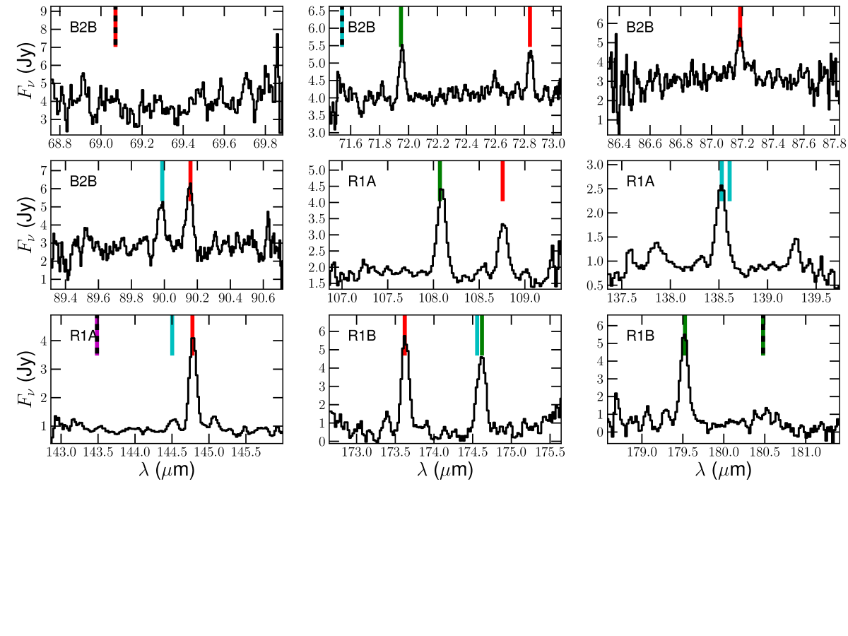
Figure 25: Line scans of V384 Per are shown in black. The vertical lines indicate molecular identifications according to Table LABEL:table:intintot2old and LABEL:table:intintot2new: CO in red, ¹³CO in magenta, ortho-H₂O in green, and para-H₂O in cyan. If a black dashed line is superimposed over the identification line, the transition was not detected by our line-fitting algorithm. The PACS band is indicated in the top left.

Figure 26: Line scans of S Aur. The line types are the same as Fig. 26.

The data have been spectrally rebinned with an oversampling factor of two, i.e. a Nyquist sampling with respect to the native instrumental resolution. We extracted the spectra from the central spaxel of every observation and applied a point-source correction. Finally, a pointing correction was applied to all MESS targets, as well as to the OT2 targets that show a continuum flux ¿ 2 Jy. Applying the pointing correction to weaker sources introduces too large an uncertainty. For these sources, we opted instead to add 5% additional flux across all line scans, which is the average flux increase introduced by the pointing correction in observations with a continuum flux ¿ 2 Jy. The data reduction has an absolute-flux-calibration uncertainty of 20%. The MESS spectra and the OT2 line scans are shown in the appendix, in Figs. 13 up to 24 and Figs. 26 up to 37, respectively.

Table 2: Properties of the sample of carbon-rich AGB stars observed with Herschel (see Sect. 2.4). The first six sources are covered in the MESS program; the rest in the OT2 program. Given per source are the IRAS number, variability type (Mira or semiregular), pulsational period ($P$), 6.3 $\mu$m flux ($F_{\mathrm{6.3\ \mu m}}$, with the suffix a for ISO SWS data and b for photometric data), adopted distance ($d$), range of distance estimates in the literature ($\Delta d$), stellar velocity with respect to the local standard of rest ($\varv_{\mathrm{LSR}}$), stellar luminosity ($L_{\star}$), stellar effective temperature ($T_{\star}$; with $\circ$ added for assumed values), gas mass-loss rate ($\dot{M}_{\mathrm{g}}$), terminal gas velocity ($\varv_{\infty\mathrm{,g}}$), and wind density tracer ($\dot{M}_{\mathrm{g}}/\varv_{\infty\mathrm{,g}}$). The source denoted with ($\star$) is of spectral type CJ and is possibly an extrinsic carbon star (Abia et al. 2010).

Star	IRAS	Var.	$P$	$F_{\mathrm{6.3\ \mu m}}$	$\varv_{\mathrm{LSR}}$	$d$	$\Delta d$	$L_{\star}$	$T_{\star}$	$\dot{M}_{\mathrm{g}}$	$\varv_{\infty\mathrm{,g}}$	$\dot{M}_{\mathrm{g}}/\varv_{\infty\mathrm{,g}}$
name	number	type	(days)	(102 Jy)	(km s-1)	(pc)	(pc)	($10^{3}$ L⊙)	(K)	($\mathrm{M}_{\odot}\ \mathrm{yr}^{-1}$)	(km s-1)	($\frac{\mathrm{M}_{\odot}\ \mathrm{yr}^{-1}}{\mathrm{km}\ \mathrm{s}^{-1}}$)
RW Lmi	10131+3049	SRa	640 (1)	25b	-1.8 (16)	410 (8)	320-710	8.3 (8)	2470 (17)	5.2$\times 10^{-6}\ {}^{(18)}$	16.5 (18)	3.2$\times 10^{-7}$
V Hya	10491-2059	SR/Mira	531 (1)	12b	-16.0 (9)	340 (6,8)	330-2160	8.3 (6)	2160 (17)	2.7$\times 10^{-6}\ {}^{(15)}$	15.0 (20)	1.8$\times 10^{-7}$
II Lup	15194-5115	Mira	580 (2)	6.0b	-15.0 (16)	640 (6)	470-640	9.1 (6)	2000 ∘	1.5$\times 10^{-5}\ {}^{(18)}$	21.0 (18)	7.0$\times 10^{-7}$
V Cyg	20396+4757	Mira	421 (1)	9.7a	15.0 (16)	420 (7)	270-740	6.6 (7)	1875 (17)	1.7$\times 10^{-6}\ {}^{(18)}$	10.5 (18)	1.6$\times 10^{-7}$
LL Peg	23166+1655	Mira	696 (2)	0.9a	-31.0 (16)	1050 (6)	950-1150	11.0 (6)	2000 ∘	1.1$\times 10^{-5}\ {}^{(18)}$	13.5 (18)	8.5$\times 10^{-7}$
LP And	23320+4316	Mira	614 (1)	4.0a	-17.0 (16)	840 (6,17)	610-870	9.7 (6)	2040 (17)	2.2$\times 10^{-5}\ {}^{(18)}$	13.5 (18)	1.6$\times 10^{-6}$
V384 Per	03229+4721	Mira	535 (1)	4.6a	-16.2 (15)	720 (6,17)	560-1060	8.4 (6)	1820 (17)	4.1$\times 10^{-6}\ {}^{(18)}$	14.5 (18)	2.8$\times 10^{-7}$
R Lep	04573-1452	Mira	427 (1)	4.0b	18.5 (12)	413 (5)	250-480	5.2 (5,6)	2290 (17)	1.3$\times 10^{-6}\ {}^{(18)}$	17.0 (12)	8.1$\times 10^{-8}$
W Ori	05028+0106	SRb	212 (1)	3.3a	18.8 (16)	377 (5)	220-460	8.0 (5,8)	2625 (17)	2.1$\times 10^{-7}\ {}^{(18)}$	12.0 (12)	1.8$\times 10^{-8}$
S Aur	05238+3406	SR/Mira	596 (1)	1.7b	-21.0 (12)	1010 (6,17)	300-1130	9.4 (6)	1940 (17)	4.5$\times 10^{-6}\ {}^{(18)}$	25.0 (12)	1.8$\times 10^{-7}$
U Hya	10350-1307	SRb	450 (1)	2.8b	-31.0 (16)	208 (5)	160-980	4.2 (5,8)	2965 (17)	1.4$\times 10^{-7}\ {}^{(18)}$	7.0 (12)	2.0$\times 10^{-8}$
QZ Mus	11318-7256	Mira	535 (1)	4.0b	-2.0 (16)	660 (6)	620-720	8.4 (6)	2200 ∘	4.8$\times 10^{-6}\ {}^{(15)}$	26.5 (15)	1.8$\times 10^{-7}$
Y CVn⋆	12427+4542	SRb	157 (1)	3.7a	21.0 (16)	320 (5)	170-340	8.7 (5,8)	2760 (17)	3.2$\times 10^{-7}\ {}^{(18)}$	8.5 (12)	3.8$\times 10^{-8}$
AFGL 4202	14484-6152	Mira	566 (3)	4.4b	24.4 (15)	611 (6,15)	570-900	8.9 (6)	2200 ∘	4.5$\times 10^{-6}\ {}^{(15)}$	19.0 (15)	2.4$\times 10^{-7}$
V821 Her	18397+1738	Mira	511 (4)	4.4b	-0.5 (16)	750 (6)	600-900	7.5 (6)	2200 ∘	2.8$\times 10^{-6}\ {}^{(18)}$	13.0 (18)	2.2$\times 10^{-7}$
V1417 Aql	18398-0220	Mira	617 (4)	4.2a	3.0 (15)	870 (6)	870-950	10.8 (6)	2000 ∘	1.7$\times 10^{-5}\ {}^{(19)}$	36.0 (15)	4.7$\times 10^{-7}$
S Cep	21358+7823	Mira	487 (1)	7.0a	-15.5 (15)	407 (5)	380-720	6.4 (5,6)	2095 (17)	1.4$\times 10^{-6}\ {}^{(18)}$	21.5 (18)	6.4$\times 10^{-8}$
RV Cyg	21412+3747	SRb	263 (1)	1.1b	17.0 (12)	640 (8)	350-850	13.4 (8)	2675 (17)	2.0$\times 10^{-7}\ {}^{(12)}$	13.0 (12)	1.5$\times 10^{-8}$

⁽¹⁾ Samus et al. (2009), ⁽²⁾ Le Bertre (1992), ⁽³⁾ Price et al. (2010), ⁽⁴⁾ Guandalini & Cristallo (2013), ⁽⁵⁾ van Leeuwen (2007), ⁽⁶⁾ Whitelock et al. (2006), ⁽⁷⁾ Whitelock et al. (2008), ⁽⁸⁾ Bergeat & Chevallier (2005), ⁽⁹⁾ Sahai et al. (2009), ⁽¹⁰⁾ Epchtein et al. (1990), ⁽¹¹⁾ Loup et al. (1993), ⁽¹²⁾ Olofsson et al. (1993), ⁽¹³⁾ Groenewegen et al. (1998), ⁽¹⁴⁾ Knapp et al. (1998), ⁽¹⁵⁾ Groenewegen et al. (2002), ⁽¹⁶⁾ De Beck et al. (2010), ⁽¹⁷⁾ Bergeat et al. (2001), ⁽¹⁸⁾ Schöier et al. (2013), ⁽¹⁹⁾ Olivier et al. (2001), ⁽²⁰⁾ Knapp et al. (1997).

2.3 Line strengths

Integrated line strengths, $I_{\mathrm{int}}$, of CO, ¹³CO, ortho-H₂O, and para-H₂O are listed in Table LABEL:table:intintmess for the MESS targets and in Tables LABEL:table:intintot2old and LABEL:table:intintot2new for the OT2 targets of the appendix. Tables LABEL:table:unidentified and LABEL:table:unidentified2 list the strengths of emission lines in the OT2 line scans that are not attributed to CO or H₂O and for which we have not attempted to identify the molecular carrier. Following Lombaert et al. (2013), the line strengths were measured by fitting a Gaussian on top of a continuum. The reported uncertainties include the fitting uncertainty and the absolute-flux-calibration uncertainty of 20%. Measured line strengths are flagged as line blends if they fulfill at least one of two criteria: 1) the full width at half maximum (FWHM) of the fitted Gaussian is larger than the FWHM of the PACS spectral resolution by at least 20%, and 2) multiple CO or H₂O transitions have a central wavelength within the FWHM of the fitted central wavelength of the emission line. In the latter case, the additional transitions contributing to the emission line are listed in Tables LABEL:table:intintmess, LABEL:table:intintot2old, and LABEL:table:intintot2new immediately below the first contributing transition. Other molecules were not considered. Because the OT2 program was specifically targeted at unblended lines based on the line survey of CW Leo, line detections in the OT2 wavelength ranges can be reliably attributed to CO and H₂O. Similarly, lines detected in the same wavelength ranges in the MESS data (given in red in Table LABEL:table:intintmess) have reliable molecular identifications. Outside these wavelength ranges, we point out that the reported line strengths not flagged as line blends may still be affected by emission from other molecules or from H₂O transitions not included in our line list (see Decin et al. 2010b for details).

2.4 Stellar and circumstellar properties

Values for several stellar and circumstellar properties were gathered from the literature and are listed in Table 2. In Sects. 4 and 5, we compare our sample of AGB sources to a set of theoretical models with a generalized set of parameters, as opposed to a tailored modeling of each source. To this end, we did not blindly assume literature values for the properties listed in Table 2, but instead carefully scaled relevant values to ensure homogeneity and consistency within the sample. In what follows, we describe this procedure where relevant. Throughout the paper, we refer to three distinct regions in the AGB wind, following Willacy & Cherchneff (1998): inner, intermediate, and outer. As a guideline, this corresponds to $r<10\ \mathrm{R}_{\star}$, $10\ \mathrm{R}_{\star}<r<100\ \mathrm{R}_{\star}$, and $r>100\ \mathrm{R}_{\star}$, respectively, for an average mass-loss rate of $\sim 10^{-6}\ \mathrm{M}_{\odot}\ \mathrm{yr}^{-1}$.

The pulsational period $P$ is taken from the General Catalog of Variable Stars (GCVS; Samus et al. 2009) when available. For the other sources, the period is taken from Le Bertre (1992), Price et al. (2010), or Guandalini & Cristallo (2013). We make use of period-luminosity $PL$-relations for both the luminosity $L_{\star}$ and the distance $d$. For the Miras, $L_{\star}$ and $d$ are taken from Whitelock et al. (2006, 2008). If not available, we use their $PL$-relation in combination with the apparent bolometric magnitude given by Bergeat et al. (2001; for LP And and V384 Per) or by Groenewegen et al. (2002; for AFGL 4202). For the SRa/b pulsators, we take $L_{\star}$ and $d$ from the PL-relation of Bergeat & Chevallier (2005). If Hipparcos parallax measurements with an uncertainty less than 40% are available, we rescale the luminosity given by these $PL$-relations to the measured distance (van Leeuwen 2007). The uncertainty on the distance estimate for the other objects is taken to be 40% owing to the broad range of distance estimates given in the literature; see column six in Table 2. To allow for a direct comparison between measured line strengths, all objects in the sample are placed at an arbitrary distance of 100 pc by rescaling the observed fluxes.

The stellar velocity $\varv_{\mathrm{LSR}}$ with respect to the local standard of rest is taken from De Beck et al. (2010). If not in their sample, it is taken from Olofsson et al. (1993) or Groenewegen et al. (2002). For the stellar effective temperature $T_{\star}$ we follow Bergeat et al. (2001), who derived relations for $T_{\star}$ versus several colors based on a sample of 54 carbon stars. However, $T_{\star}$ is notoriously difficult to constrain for stars with a large infrared (IR) excess. For this reason, the reddest carbon stars are absent in the sample of Bergeat et al. (2001). Two of these absent sources, II Lup and LL Peg, are included in the classification of cool carbon variables (CVs) of Knapik et al. (1999) as CV7 objects, as they have the reddest spectral energy distribution (SED) among carbon stars. The average effective temperature attributed by Bergeat et al. (2001) to the CV7 class is 2000 K, which we adopt for II Lup and LL Peg, as well as for V1417 Aql, which has an IR color similar to II Lup and LL Peg. While bluer than II Lup, LL Peg, and V1417 Aql, the remaining objects still show relatively red IR colors and have intermediate-to-high mass-loss rates. Hence, we assume they are either CV6 or CV7, to which Bergeat et al. (2001) assign a temperature range of 2000-2400 K. We do not take into account time-dependent variations in stellar parameters. We therefore assume $R_{\star}$ to be the stellar radius associated with a blackbody radiator, following the Stefan-Boltzmann relation. Taking into account that $L_{\star}$ gives an average stellar luminosity scaled with distance through the $PL$-relations, $R_{\star}$ should give a reasonable estimate of the average stellar radius.

A broad range of gas mass-loss rates $\dot{M}_{\mathrm{g}}$ can be found in the literature for all objects in the sample, derived from either low-$J$ CO emission lines or SED modeling. We only use $\dot{M}_{\mathrm{g}}$ estimates derived from CO modeling because mass-loss rates derived from modeling the thermal dust emission require a conversion using a dust-to-gas ratio, which introduces a large uncertainty. $\dot{M}_{\mathrm{g}}$ values derived from CO lines do depend on the CO abundance with respect to H₂ ($n_{\mathrm{CO}}/n_{\mathrm{H}_{2}}$), a parameter that is also not well constrained. In Sect. 4.3 we show that the impact of the CO abundance is limited in the context of the constraints that we have from chemical models. To maintain consistency, we rescale quoted mass-loss rates in the literature based on the distance $d_{\mathrm{lit}}^{2}$ for which they were derived to the distance used here (see column 7 in Table 2 by applying the scaling factor $d^{2}$/$d_{\mathrm{lit}}^{2}$; Ramstedt et al. 2008, De Beck et al. 2010). Most values for $\dot{M}_{\mathrm{g}}$ were taken from the recent work by Schöier et al. (2013). Other values are taken from Groenewegen et al. (2002), Olivier et al. (2001), or Olofsson et al. (1993). The uncertainty on $\dot{M}_{\mathrm{g}}$ amounts to a factor of three. The gas terminal velocity $\varv_{\infty\mathrm{,g}}$ is taken from Olofsson et al. (1993), Groenewegen et al. (2002), and Schöier et al. (2013). The uncertainty on $\varv_{\infty\mathrm{,g}}$ is usually not more than 10%. The final column of Table 2 lists values for $\dot{M}_{\mathrm{g}}/\varv_{\infty\mathrm{,g}}$, which is a quantity that we use as a density tracer (see, e.g., Ramstedt et al. 2009). The uncertainty on $\dot{M}_{\mathrm{g}}/\varv_{\infty\mathrm{,g}}$ is dominated by the uncertainty on $\dot{M}_{\mathrm{g}}$.

To have an indicator for the dust content of the stellar wind and because of its relevance for H₂O excitation (see Sect. 4.2), we list the measured 6.3 $\mu$m flux for each source in Jansky (not distance scaled). These are taken from ISO-SWS spectra if available. In all other cases, the values are derived from an interpolation of photometric measurements at shorter and longer wavelengths.

2.5 V Hya and S Aur

A special note is warranted for V Hya, which is suggested to be in transition between the AGB stage and the planetary nebula stage (e.g., Knapp et al. 1997, Sahai et al. 2003, Sahai et al. 2009). Clearly, V Hya does not necessarily follow the general trends observed in other semiregular AGB stars. An indication for this is a stellar luminosity of $17.9\times 10^{3}$ L_⊙ derived from the $PL$-relation of Bergeat & Chevallier (2005), which is unusually high for a carbon AGB star (see, e.g., the overview in Fig. C.2. of De Beck et al. 2010, and the luminosity function in Fig. 4 of Guandalini & Cristallo 2013). The Mira $PL$-relation of Whitelock et al. (2006), which we adopted, instead leads to $L_{\star}=8.3\times 10^{3}$ L_⊙, in agreement with many other studies dedicated to the peculiar kinematic structure of this source. The use of the Mira $PL$-relation is further supported by the findings of Knapp et al. (1999), who suggest V Hya may be a Mira. Additionally, most of the kinematic complexity in V Hya occurs in the outer circumstellar wind where multiple components in the kinematic structure are observed in the low-$J$ CO emission lines, including a high-velocity bipolar outflow. CS and HC₃N emission lines, which are formed in the inner or intermediate wind, show only one component with an expansion velocity of $\sim 15$ km s^-1 (Knapp et al. 1997), indicating that their formation region behaves more like a normal spherically symmetric AGB wind. Most lines detected in the PACS wavelength range are formed in this region. We take $\varv_{\mathrm{LSR}}=-16.0$ km s^-1 from Sahai et al. (2009).

There is some debate whether S Aur is a semiregular variable or a Mira. The GCVS catalog lists S Aur as a semiregular, but the light curve amplitude in $V$ is $>2.5$ mag, categorizing it as a Mira variable. Moreover, the effective temperature of S Aur ($T_{\star}=1940$ K) is extremely low, and therefore more reminiscent of Miras than semiregulars. Because there is no a priori reason to assume that S Aur is a semiregular, we treat the source as a Mira for the distance and luminosity determination. We note that, in the discussion of the importance of variability in SRa sources, the variability type for both V Hya and S Aur is debatable.

3 Trend analysis

To determine dependencies of the H₂O abundance on stellar and/or circumstellar properties, we combine two methods. In this section, we look for empirical correlations between observed molecular-emission line strengths and mass-loss rate. In Sect. 4 and 5, we perform a parameter study by calculating a grid of theoretical radiative-transfer models to compare with the measured line strengths. This combined approach allows us to identify model-independent H₂O emission trends and to disentangle radiative-transfer effects from other effects that contribute to the observed correlations.

3.1 The observed CO line strength as an H₂ density tracer

Because one of the goals of this study is to constrain the H₂O abundance with respect to H₂ ($n_{\mathrm{H}_{2}\mathrm{O}}/n_{\mathrm{H}_{2}}$) in the sample sources, the ratio $I_{\mathrm{H}_{2}\mathrm{O}}/\dot{M}_{\mathrm{g}}$ is of interest as the H₂O number density is proportional to $I_{\mathrm{H}_{2}\mathrm{O}}$ and the H₂ number density to $\dot{M}_{\mathrm{g}}$. However, large uncertainties affect this ratio, owing to the uncertainties on the mass-loss rate itself and to the distance scaling that is necessary to compare the measurements within the sample. As such, considering line-strength ratios rather than line strengths is preferred, as these are distance independent. An interesting line-strength ratio is H₂O/CO, which provides an H₂O abundance proxy via

$$I_{\mathrm{H}_{2}\mathrm{O}}/I_{\mathrm{CO}}\sim n_{\mathrm{H}_{2}\mathrm{O}}/n_{\mathrm{CO}}=(n_{\mathrm{H}_{2}\mathrm{O}}/n_{\mathrm{H}_{2}})\times(n_{\mathrm{H}_{2}}/n_{\mathrm{CO}}),$$

assuming that CO has a constant molecular abundance with respect to H₂ throughout the entire wind, up to the photodissociation radius, and in the absence of optical-depth effects.

Table 3: CO transitions selected for this study based on the wavelength ranges of the OT2 line scans. Given are the central wavelength ($\lambda_{0}$), upper-level energy ($E_{\mathrm{u}}$), and number of targets with a detection ($n$) of the emission line.

Molecule	Transition	$\lambda_{0}$ ($\mu$m)	$E_{\mathrm{u}}$ (cm-1)	$n$
12CO	$J=15-14$	173.6	461.1	18
	$J=18-17$	144.8	656.8	18
	$J=24-23$	108.8	1151	18
	$J=29-28$	90.2	1668	18
	$J=30-29$	87.2	1783	17
	$J=36-35$	72.8	2550	10
	$J=38-37$	69.1	2836	8
13CO	$J=19-18$	143.5	697.6	8

Seven CO transitions and one ¹³CO transition have been observed in the wavelength ranges of the OT2 line scans. We limit our study to these transitions because a maximum of only six detections are available for the other CO transitions from the MESS data, and some of those lines may be affected by line blending. An overview of the relevant CO transitions is given in Table 3. Fig. 1 shows the measured line strengths of CO $J=15-14$, scaled to a distance of 100 pc. A correlation between line strength and mass-loss rate is present, which is expected considering that the mass-loss rates listed in Table 2 are exclusively derived from CO emission lines. Because CO is predominantly excited through collisions with H₂, CO is a reliable tracer of $\dot{M}_{\mathrm{g}}$ and, hence, of $n_{\mathrm{H}_{2}}$. At the high end of the range of mass-loss rate, the trend flattens off where the lines become optically thick. We show in Sect. 4.3 that theoretical models recover this behavior. For higher-$J$ levels the flattening of the slope sets in at a lower mass loss because the lines are formed closer to the stellar surface, where the gas density is higher. Therefore, the $J=15-14$ transition is best suited to act as an H₂ density tracer. CO $J=15-14$ has been detected in all objects in the sample, and none of them are flagged as a line blend.

As shown in Fig 1, the Miras and SRa sources cannot be distinguished based on CO line strength. The SRb sources cluster at the low end of the range of mass-loss rate, but still seem to follow the linear trend set by the Miras and SRa sources. Studies on large populations have shown that Miras are considered to be fundamental-mode pulsators, while semiregulars are overtone pulsators or short-period fundamental-mode pulsators (Wood et al. 1999; Wood 2010). The differentiation between SRa and SRb variables is based on the regularity of the light curves of these sources, but no definite conclusion can be drawn about the pulsational mode they exhibit. As shown by Bowen (1988), overtone pulsators are significantly less efficient at driving a stellar wind than fundamental-mode pulsators. If one assumes that SRa sources pulsate in a short-period fundamental mode, and SRb sources in a first or second overtone, this could explain the clear difference in terms of mass-loss rate between these two variability classes. Another suggestion is that SRb sources are unstable in more than one pulsation mode, and thus experience more than one pulsation period characteristic of each mode, explaining the lower periodicity of their light curves (Soszyński & Wood 2013). This may also decrease the efficiency with which a wind is driven. We recall that two out of the three SRa sources in our sample have a debatable variability type and were treated as Miras for the luminosity and distance determination.

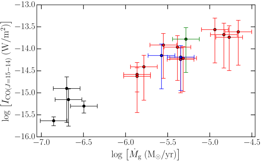
Figure 1: Line strengths of the CO $J=15-14$ transition as a function of the mass-loss rate $\dot{M}_{\mathrm{g}}$. The data points are color coded according to the variability type: Miras in red, SR/Mira sources in blue, the SRa source in green, and SRb sources in black. The line strengths are scaled to a distance of 100 pc.

3.2 The H₂O/CO line-strength ratio versus $\dot{M}_{\mathrm{g}}$

We only take the H₂O transitions in the wavelength ranges of the OT2 line scans into account. Their central wavelengths and upper-level energies are listed in the first columns of Table 4. Two additional transitions, with higher upper-level energies, are included in Table LABEL:table:intintot2old and LABEL:table:intintot2new, but both occur in a blend with another H₂O transition listed in Table 4 and do not contribute significantly to the emission. We do not consider them in the remainder of this study. In what follows, we primarily look at the H₂O $J_{\mathrm{K}_{\mathrm{a}},\mathrm{K}_{\mathrm{c}}}=2_{1,2}-1_{0,1}$ line because it is the only H₂O line detected in the entire sample.

Table 4: H₂O transitions selected for this study. Given are the central wavelength ($\lambda_{0}$), upper-level energy, ($E_{\mathrm{u}}$) and number of targets with a detection ($n$) of the emission line. Also given for each transition are the empirical fitting results of the linear correlation $Y=\bar{a}+\bar{b}X$ between the H₂O/CO line-strength ratio and the mass-loss rate. $n_{\mathrm{inc}}=n-n_{\mathrm{SRb}}$ gives the number of detections included in the fit, $\bar{a}$ and $\bar{b}$ the mean coefficients, $\sigma_{\mathrm{\bar{a}}}$ and $\sigma_{\mathrm{\bar{b}}}$ the fitting uncertainties on both coefficients, and $\sigma_{\mathrm{\bar{a}\bar{b}}}$ the covariance between the two. The middle five columns assume the logarithm of the line-strength ratio as the independent variable ($X$) and the logarithm of the mass-loss rate as the variable ($Y$), while the last five columns give the results for the inverse relation. The trends are valid for the subsample of Miras and SRa sources only; see Sect. 3.2.

Molecule	Transition	$\lambda_{0}$ ($\mu$m)	$E_{\mathrm{u}}$ (cm-1)	$n$	$n_{\mathrm{inc}}$	$\bar{a}$	$\sigma_{\mathrm{\bar{a}}}$	$\bar{b}$	$\sigma_{\mathrm{\bar{b}}}$	$\sigma_{\mathrm{\bar{a}\bar{b}}}$	$\bar{a}$	$\sigma_{\mathrm{\bar{a}}}$	$\bar{b}$	$\sigma_{\mathrm{\bar{b}}}$	$\sigma_{\mathrm{\bar{a}\bar{b}}}$
o-H2O	$J_{\mathrm{K}_{\mathrm{a}},\mathrm{K}_{\mathrm{c}}}=2_{2,1}-2_{1,2}$	180.5	134.9	11	11	-5.9	0.3	-0.9	0.4	0.12	-2.1	0.7	-0.25	0.12	0.08
	$J_{\mathrm{K}_{\mathrm{a}},\mathrm{K}_{\mathrm{c}}}=2_{1,2}-1_{0,1}$	179.5	79.5	18	14	-5.51	0.07	-0.8	0.2	0.012	-2.2	0.6	-0.38	0.11	0.06
	$J_{\mathrm{K}_{\mathrm{a}},\mathrm{K}_{\mathrm{c}}}=3_{0,3}-2_{1,2}$	174.6	136.8	12	9	-5.70	0.13	-0.8	0.3	0.03	-2.8	0.8	-0.45	0.16	0.13
	$J_{\mathrm{K}_{\mathrm{a}},\mathrm{K}_{\mathrm{c}}}=2_{2,1}-1_{1,0}$	108.1	134.9	17	13	-5.42	0.06	-0.7	0.2	0.004	-2.1	0.7	-0.38	0.12	0.08
	$J_{\mathrm{K}_{\mathrm{a}},\mathrm{K}_{\mathrm{c}}}=7_{0,7}-6_{1,6}$	72.0	586.2	13	12	-5.59	0.09	-0.7	0.2	0.017	-2.5	0.7	-0.41	0.14	0.10
	$J_{\mathrm{K}_{\mathrm{a}},\mathrm{K}_{\mathrm{c}}}=3_{3,0}-2_{2,1}$	66.4	285.4	15	12	-5.32	0.06	-0.8	0.3	-0.005	-1.3	0.6	-0.26	0.11	0.06
p-H2O	$J_{\mathrm{K}_{\mathrm{a}},\mathrm{K}_{\mathrm{c}}}=4_{1,3}-3_{2,2}$	144.5	275.5	8	8	-5.9	0.3	-0.5	0.3	0.09	-2.8	1.2	-0.3	0.2	0.3
	$J_{\mathrm{K}_{\mathrm{a}},\mathrm{K}_{\mathrm{c}}}=3_{1,3}-2_{0,2}$	138.5	142.3	17	13	-5.68	0.11	-0.9	0.2	0.02	-2.5	0.6	-0.39	0.12	0.07
	$J_{\mathrm{K}_{\mathrm{a}},\mathrm{K}_{\mathrm{c}}}=3_{2,2}-2_{1,1}$	90.0	206.3	15	14	-5.60	0.11	-0.5	0.2	0.02	-2.3	0.8	-0.34	0.15	0.12
	$J_{\mathrm{K}_{\mathrm{a}},\mathrm{K}_{\mathrm{c}}}=7_{1,7}-6_{0,6}$	71.5	586.4	8	7	-5.7	0.2	-0.7	0.4	0.08	-2.3	1.0	-0.33	0.19	0.19

Fig. 2 shows the line-strength ratio of H₂O $J_{\mathrm{K}_{\mathrm{a}},\mathrm{K}_{\mathrm{c}}}=2_{1,2}-1_{0,1}$ and CO $J=15-14$ as a function of the mass-loss rate. Several qualitative conclusions can be drawn. A downward trend toward higher mass-loss rate is present in the H₂O/CO line-strength ratios, indicated by the green arrow superimposed on the data points (see Sect. 3.3). Assuming H₂O is homogeneously distributed within the formation region of a given line, this suggests that the H₂O abundance also decreases with increasing mass-loss rate in the same fashion. Fig. 2 shows the line-strength ratios for only one H₂O line, but the trend is significant for other H₂O lines as well (see Sect. 3.3). However, contrary to the CO line strengths, the H₂O/CO line-strength ratios of the low-$\dot{M}_{\mathrm{g}}$ SRb sources do not follow the trend set by the Miras and SRa sources. Instead, they group together at the low end of the range of mass-loss rate featuring low line-strength ratios. Though only four sources can be considered, of which one is flagged as a line blend (see Sect. 2.3 for clarification), a tentative upward trend between the H₂O/CO line-strength ratio and the mass-loss rate appears present within the SRb sample.

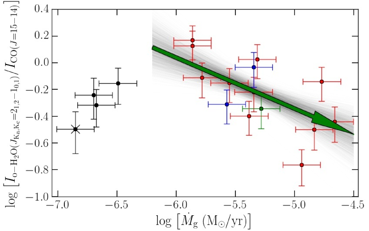
Figure 2: Line-strength ratio of the H₂O $J_{\mathrm{K}_{\mathrm{a}},\mathrm{K}_{\mathrm{c}}}=2_{1,2}-1_{0,1}$ transition and CO $J=15-14$ transition as a function of the mass-loss rate $\dot{M}_{\mathrm{g}}$. The data points are color coded according to the variability type: Miras in red, SR/Mira sources in blue, the SRa source in green, and SRb sources in black. A black cross superimposed on a point indicates that the H₂O line strength is flagged as a blend (see Sect. 2.3 for clarification). The gray lines show the individual Monte Carlo linear fitting results to the data points for Miras and SRa sources. The green arrow indicates the mean linear relation (see Sect. 3.3).

The difference between the SRb sources, on the one hand, and the Miras and SRa sources, on the other hand, suggests some dependence of H₂O emission on pulsational properties. Fig. 3 gives the line-strength ratio of the H₂O $J_{\mathrm{K}_{\mathrm{a}},\mathrm{K}_{\mathrm{c}}}=2_{1,2}-1_{0,1}$ transition and the CO $J=15-14$ transition as a function of pulsational period. The data points are color coded according to the wind density tracer $\dot{M}_{\mathrm{g}}/\varv_{\infty\mathrm{,g}}$. The Miras and SRa sources are shown in blue, red, and green for increasing $\dot{M}_{\mathrm{g}}/\varv_{\infty\mathrm{,g}}$ (as indicated in the legend). An increasing outflow density, and thus a decreasing H₂O/CO line-strength ratio, is associated with an increasing pulsational period. The pulsational period and mass-loss rate were derived independently (see Table 2 for references.) This supports previous theoretical (Bowen 1988) and observational (Wood et al. 2007; De Beck et al. 2010) studies that have shown a strong correlation between the mass-loss rate and the pulsational period of AGB stars. The SRb sources (shown in black in Fig. 3) do not show a clear-cut correlation between wind density and pulsational period. We note that the H₂O $J_{\mathrm{K}_{\mathrm{a}},\mathrm{K}_{\mathrm{c}}}=2_{1,2}-1_{0,1}$ transition detected in U Hya (the right most black point in Fig. 3) is flagged as a line blend, which effectively makes the H₂O/CO line-strength ratio an upper limit.

Figure 3: Line-strength ratio of the H₂O $J_{\mathrm{K}_{\mathrm{a}},\mathrm{K}_{\mathrm{c}}}=2_{1,2}-1_{0,1}$ transition and the CO $J=15-14$ transition as a function of the pulsational period. The points with error bars give the measured H₂O/CO line-strength ratios, color coded according to the value of the wind density proxy $\dot{M}_{\mathrm{g}}/\varv_{\infty\mathrm{,g}}$ in units of $\mathrm{M}_{\odot}\ \mathrm{yr}^{-1}\ \mathrm{km}^{-1}\ \mathrm{s}$ (see legend). A black cross superimposed on the data point indicates that the H₂O line is flagged as a blend.

3.3 Least-squares fitting approach

To quantify the negative correlation between measured H₂O/CO line-strength ratios and mass-loss rates of the Miras and the SRa sources, we apply a least-squares fitting technique to fit a linear function in logarithmic scale. Measurements are included only when $\dot{M}_{\mathrm{g}}>5\times 10^{-7}$ $\mathrm{M}_{\odot}\ \mathrm{yr}^{-1}$. This removes the four SRb sources from the statistical sample. We have to take into account the uncertainties on the measured values, which follow a normal distribution in linear space, and the uncertainty on the mass-loss rate to assess the accuracy of the fitted slope and intercept. Studies investigating the mass-loss rate of AGB outflows typically report uncertainties of a factor of three (Ramstedt et al. 2008; De Beck et al. 2010; Lombaert et al. 2013; Schöier et al. 2013). For our purposes, we assume that the derived $\dot{M}_{\mathrm{g}}$ values follow a normal distribution in logarithmic scale with the 3$\sigma$-confidence level equal to this factor of three accuracy.

To ensure a proper error propagation, we apply a Monte Carlo-like approach, in which we draw a large number of guesses ($N=10^{6}$) for the relevant quantities from their respective distributions. Since we fit the observed line-strength ratios in logarithmic scale, we can also apply this approach to the mass-loss rate, for which we draw the guess from the normal distribution of logarithmic values. This results in $N$ linear relations from which we calculate the mean slope and intercept to arrive at a mean relation between the relevant quantities. At the same time, we also determine whether the slope and intercept of the $N$ relations are correlated. This approach is applied to all H₂O transitions. The number of data points $n$ per transition taken into account for the linear fit is given in column 5 of Table 4. The mean coefficients $\bar{a}$ and $\bar{b}$ of the linear relation $Y=\bar{a}+\bar{b}X$ between $I_{\mathrm{H}_{2}\mathrm{O}}/I_{\mathrm{CO}}$ and $\dot{M}_{\mathrm{g}}$ are listed in the next ten columns of Table 4; their uncertainties and the covariance between them are also listed. We give the results for $I_{\mathrm{H}_{2}\mathrm{O}}/I_{\mathrm{CO}}$ as independent variable $X$ in columns 6 through 10 and the results for the inverse relation in columns 11 through 15. Taking the reciprocal of one relation does not necessarily result in the coefficients of the inverse relation because the least-squares minimization only takes the vertical residuals between the data points and the best linear fit into account. The $N$ individual linear fit results in the Monte Carlo approach are shown in gray-black in Fig. 2. The green arrow indicates the mean linear relation according to the coefficients given in Table 4 for the H₂O $J_{\mathrm{K}_{\mathrm{a}},\mathrm{K}_{\mathrm{c}}}=2_{1,2}-1_{0,1}$ transition.

Notably, within the fitting uncertainties, the slope of the linear relation is similar for all ortho- and para-H₂O lines. We list the covariance between the slope and the intercept of the linear relation as well, which is a measure of how closely correlated the slope and the intercept are. With the exception of one, all relations listed in Table 4 show a strong correlation between the slope and the intercept, meaning that a larger intercept must be associated with a steeper slope. This is evidenced by the gray lines in Fig. 2, which seem to knot together in the intermediate $\dot{M}_{\mathrm{g}}$ region, while spreading out for more extreme values of $\dot{M}_{\mathrm{g}}$. The H₂O/CO line-strength ratio for the $J_{\mathrm{K}_{\mathrm{a}},\mathrm{K}_{\mathrm{c}}}=3_{3,0}-2_{2,1}$ transition is attributed to a small negative covariance when taking $I_{\mathrm{H}_{2}\mathrm{O}}/I_{\mathrm{CO}}$ as the independent variable $X$. This suggests that the slope and intercept of the linear relation are weakly correlated, hence the negative value. However, the slope-intercept correlation is very weak for this particular transition because of a large scatter between the data points. As such, the linear fit to this H₂O/CO line-strength ratio and the mass-loss rate is less reliable, but still confirms the observed downward trend based on the negative slope $\bar{b}=-0.8$.

The relations in columns 6 through 10 can serve as a mass-loss indicator as long as measurements for the relevant H₂O and CO line strengths are available. The relations in columns 11 through 15 are helpful in predicting the H₂O/CO line-strength ratio, given a mass-loss rate. When using these relations to estimate a mass-loss rate or predict a line-strength ratio, the uncertainty on the result can be determined from the relation

$$\sigma_{\rm Y}=\sqrt{\sigma_{\rm\bar{a}}^{2}+\bar{b}^{2}\sigma_{\rm X}^{2}+X^{2}\sigma_{\rm\bar{b}}^{2}+X\sigma_{\rm\bar{a}\bar{b}}^{2}}.$$

Barring systematic effects in the assumed $\dot{M}_{\mathrm{g}}$ values for our sample, this leads to an uncertainty of about 0.3 dex on the logarithmic values.

Table 5: Stellar and circumstellar parameters of the model grid described in Sect 4.1. The first and second column list the parameter and its unit, the third column lists the adopted value in the standard model grid, the fourth column indicates the sampling range in which an individual parameter is allowed to vary, and the last column gives the step size with which the parameter was probed. Listed are the gas mass-loss rate ($\dot{M}_{\mathrm{g}}$), H₂O abundance with respect to molecular hydrogen ($n_{\mathrm{H}_{2}\mathrm{O}}/n_{\mathrm{H}_{2}}$), power of the adopted radial gas kinetic-temperature profile given in Eq. 1 ($\epsilon$), effective temperature ($T_{\star}$), luminosity ($L_{\star}$), gas terminal velocity ($\varv_{\infty\mathrm{,g}}$), dust-to-gas ratio ($\psi$), and CO abundance with respect to molecular hydrogen ($n_{\mathrm{CO}}/n_{\mathrm{H}_{2}}$).

Parameter	Unit	Standard	Range	Step size
$\log(\dot{M}_{\mathrm{g}})$	$\mathrm{M}_{\odot}\ \mathrm{yr}^{-1}$		$[-8.0,-4.5]$	0.5
$\log($$n_{\mathrm{H}_{2}\mathrm{O}}/n_{\mathrm{H}_{2}}$)			$[-10,-4]$	1
$\epsilon$		0.4	$[0.3,0.9]$	0.1
$T_{\star}$	$10^{3}$ K	2.4	$[2.4,3.0]$	0.3
$L_{\star}$	103 L⊙	8	$[4,12]$	4
$\varv_{\infty\mathrm{,g}}$	km s-1	10	$[10,25]$	5
$\log(\psi)$		-3	$[-3.3,-2.7]$	0.3
$n_{\mathrm{CO}}/n_{\mathrm{H}_{2}}$	$10^{-3}$	0.8	$[0.6,1.2]$	0.2

4 Sample-wide H₂O abundance

A negative correlation between the H₂O/CO line-strength ratio and the mass-loss rate is evident for the Miras and SRa sources. We compute a set of radiative-transfer models to investigate the role of optical-depth effects and to establish whether or not this points to a negative correlation between the H₂O abundance and mass-loss rate. Because modeling the line strengths for each source individually is beyond the scope of this study, we opt for an approach in which we calculate these line strengths for models covering the parameter range appropriate for Miras, SRa, and SRb sources.

4.1 The model grid

We set up a model grid with a fine sampling of the H₂O abundance, the mass-loss rate $\dot{M}_{\mathrm{g}}$, and the gas temperature profile $T_{\mathrm{g}}(r)$, and with a coarse sampling of the other stellar and circumstellar properties: the gas terminal velocity $\varv_{\infty\mathrm{,g}}$, the stellar effective temperature $T_{\star}$, the stellar luminosity $L_{\star}$, the dust-to-gas ratio $\psi$, and the CO abundance with respect to molecular hydrogen. We refer to a single set of values for the latter set of properties as the standard model grid, for which the values are listed in Table. 5, and we represent it by a black curve in the figures in Sect. 4 for clarity. In this grid, the mass-loss rate and the H₂O abundance are allowed to vary between $1\times 10^{-8}\ \mathrm{M}_{\odot}\ \mathrm{yr}^{-1}$ and $3\times 10^{-5}\ \mathrm{M}_{\odot}\ \mathrm{yr}^{-1}$, and $10^{-10}$ and $10^{-4}$, respectively. To probe the sensitivity of the observed H₂O emission to the other stellar and circumstellar properties, we created secondary model grids in which at most one additional fixed parameter from the standard grid was allowed to vary. We consider each grid separately in Sects. 4.3 and 4.4. Table 5 lists both the adopted value for the standard model grid as well as the sampling range and step size of the parameters. Beam effects or other telescope-related properties have been corrected for during the PACS data reduction, such that measured line strengths can be directly compared with the intrinsic line strengths of theoretical predictions. This assumes that the PACS observations are not spatially resolved, which has been one of our target selection criteria (see Sect. 2.1). Unfortunately, even though it is the prototypical carbon-rich AGB star, CW Leo has to be excluded from the sample as a result of its spatial extent as observed by the PACS instrument. We refer to the work by Cernicharo et al. (2014) for typical CO and H₂O line strengths, but we caution that these values must be rescaled to 100 pc to facilitate a comparison with our results, which is not straightforward given CW Leo’s extension.

We calculate spectral line profiles using GASTRoNOoM (Decin et al. 2006, 2010b; Lombaert et al. 2013). In these calculations, the density distribution of the outflow is assumed to be smooth and spherically symmetric, i.e. we do not take a small-scale structure in the form of clumps or a large-scale structure in the form of a disk or polar outflows into account. We do not take masing into account in our modeling. We use a COMARCS synthetic spectrum for the central star (Aringer et al. 2009) with $log(g)=0.0$, a C/O ratio of 1.4, $M_{\star}=1.0$ M_⊙, a microturbulent velocity of 2.5 km s^-1, and solar metallicity. For CO, we take transitions in the ground- and first-vibrational state up to $J=60$ into account. The energy levels, transition frequencies, and Einstein A coefficients were taken from Goorvitch & Chackerian (1994) and the CO-H₂ collision rates from Larsson et al. (2002) (see Appendix A in Decin et al. 2010b for more details). For H₂O, we take into account the 45 lowest levels of the ground state and the $\nu_{2}=1$ and $\nu_{3}=1$ vibrationally excited states. Level energies, frequencies, and Einstein A coefficients were taken from the HITRAN water line list (Rothman et al. 2009), and H₂O-H₂ collisional rates from Faure et al. (2007) (see Decin et al. 2010b, and Appendix B in Decin et al. 2010c for more details). Recently, Dubernet et al. (2009) and Daniel et al. (2011) published new H₂O-H₂ collisional rates. Daniel et al. (2012) compared these collision rates to those from Faure et al. (2007) and found that the line strengths can be affected by up to a factor of 3 for low H₂O abundance ($n_{\mathrm{H}_{2}\mathrm{O}}/n_{\mathrm{H}_{2}}$ $\sim 10^{-8}$) and low density ($n_{\mathrm{H}_{2}}<10^{7}$) regimes. They also note that when H₂O excitation is dominated by pumping via the dust radiation field, these differences are attenuated. Hence, we do not expect this to affect our results significantly.

The molecular abundances with respect to H₂ of both CO and H₂O are assumed to be constant throughout the wind up to the photodissociation radius where interstellar UV photons destroy the molecules. The CO photodissociation radius is set by the formalism of Mamon et al. (1988). For H₂O we use the analytic formula from Groenewegen (1994). The acceleration of the wind to the terminal expansion velocity $\varv_{\infty\mathrm{,g}}$ of the gas is set by momentum transfer from dust to gas, assuming full momentum coupling between the two components (Kwok 1975). The gas turbulent velocity $\varv_{\mathrm{stoch}}$ is fixed at 1.5 km s^-1. Because the cooling contribution from HCN is not well constrained (Decin et al. 2010b; De Beck et al. 2012), we approximate the gas kinetic-temperature structure with a power law of the form

$$T_{\mathrm{g}}(r)=T_{\star}\ \left(\frac{r}{R_{\star}}\right)^{-\epsilon},$$ (1)

where $r$ is the distance to the center of the star. As shown by Lombaert et al. (2013), dust can play an important role in H₂O excitation. Following Lombaert et al. (2012), we use a distribution of hollow spheres (DHS, Min et al. 2003) with filling factor 0.8 to represent the dust extinction properties, a dust composition that is 75% amorphous carbon, 10% silicon carbide, and 15% magnesium sulfide, and assume composite dust grains, leading to thermal equilibrium between all three dust species. The optical properties used to calculate the extinction contribution from these species are taken from Jäger et al. (1998), Pitman et al. (2008), and Begemann et al. (1994), respectively. We take the inner radius of the dusty circumstellar envelope to match the dust condensation radius, which is determined following Kama et al. (2009) with use of the dust radiative-transfer code MCMax (Min et al. 2009). Typical inner-radius values lie between 2 and 2.5 R_⋆.

4.2 The 6.3 $\mu$m flux

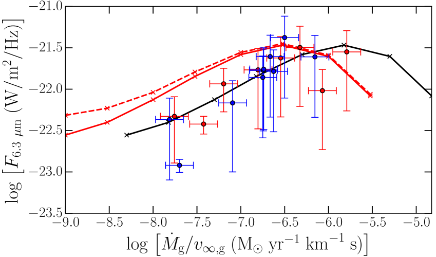
Figure 4: Fluxes at 6.3 $\mu$m as a function of $\dot{M}_{\mathrm{g}}/\varv_{\infty\mathrm{,g}}$. The data points are color coded according to the method with which the 6.3 $\mu$m flux was measured: from ISO data in red, and interpolation of photometric data points in blue. The full and dashed lines are fluxes calculated from models. The red lines represent models with $\psi=0.005$, while the black line shows models with $\psi=0.001$. The dashed line makes use of a blackbody spectrum of 2400 K for the central star, while the full lines use a COMARCS spectrum. The 6.3 $\mu$m fluxes are scaled to a distance of 100 pc.

The excitation analysis of H₂O is important when considering H₂O emission from any type of source. We refer to González-Alfonso et al. (2007), Maercker et al. (2008), and Lombaert et al. (2013) for examples of overviews of the most important excitation channels for H₂O. These include: 1) collisional excitation; 2) radiative vibrational excitation in the near- and mid-IR; and 3) radiative rotational excitation in the mid- and far-IR. The $\nu_{2}=1$, $\nu_{1}=1$, and $\nu_{3}=1$ vibrational states can be accessed by absorption of radiation at about 6.3 $\mu$m and 2.7 $\mu$m, respectively. Especially the $\nu_{2}=1$ state was shown to have a strong impact on the excitation of H₂O molecules by González-Alfonso et al. (2007). We therefore carefully consider whether our modeling approach correctly reproduces the observed flux at 6.3 $\mu$m for our sample.

The stellar spectrum and the presence of dust primarily determine the flux at 6.3 $\mu$m. Atmospheric absorption bands can have a significant impact on the near-IR flux. For this reason, we make use of a COMARCS synthetic spectrum as opposed to a blackbody spectrum for a more reliable estimate of the stellar flux at 6.3 $\mu$m. This flux depends on the pulsational phase of the star, which is not taken into account in the COMARCS models (e.g., De Beck et al. 2012 for CW Leo). Time-dependent modeling of the atmosphere and inner wind is beyond the scope of this work.

$\begin{array}[]{cc}\leavevmode\resizebox{256.0748pt}{}{\includegraphics{covshellmass_eps.pdf}}&\leavevmode\resizebox{256.0748pt}{}{\includegraphics{covshellmass_hot_eps.pdf}}\end{array}$

Figure 5: Line strengths of two CO transitions as a function of $\dot{M}_{\mathrm{g}}/\varv_{\infty\mathrm{,g}}$: CO $J=15-14$ on the left and CO $J=30-29$ on the right. The points with error bars give the measured CO line strengths, color coded according to the variability type. A black cross superimposed on the data point indicates that the CO line is flagged as a blend. The colored curves show the predicted CO line strength for various values of the temperature power law exponent $\epsilon$. Adopted values for other parameters are listed in Table 5. The line strengths are scaled to a distance of 100 pc.

The presence of dust reddens the stellar spectrum and affects the radiation field that H₂O is subjected to. The amount of reddening depends critically on the optical depth in the dust continuum. Reddening has two major effects. Firstly, a higher dust content smooths out the stellar spectrum. In other words, using a synthetic spectrum rather than a blackbody spectrum becomes irrelevant for high mass-loss rates. Secondly, the spectral reddening shifts a large portion of the emitted photons away from the near-IR to the mid-IR. In first order, the 2.7 $\mu$m H₂O vibrational excitation channels become less relevant for higher mass-loss rates. Once $\dot{M}_{\mathrm{g}}$ is high enough to turn the star into an extreme carbon star (e.g., in the case of LL Peg, where the 11-$\mu$m SiC feature is in absorption; see, for instance, Lombaert et al. 2012) the 6.3 $\mu$m H₂O vibrational excitation channel loses importance as well, in favor of the far-IR rotational excitation channels of H₂O.

To illustrate these effects, Fig. 4 shows the predicted and measured 6.3 $\mu$m fluxes for our sample of carbon stars scaled to a distance of 100 pc. The uncertainties on the observed fluxes are predominated by the uncertainty on the distance. The models are calculated for a blackbody and a COMARCS stellar spectrum of $T_{\star}=2400$ K, for two different dust-to-gas ratios: the canonical value of 0.005 and a value of 0.001. The 6.3 $\mu$m flux is only weakly dependent on the stellar spectrum in the low mass-loss rate regime. The dust-to-gas ratio has a much more pronounced effect across all densities. The overall trend supports $\psi=0.001$. For reference, the dust opacity at 6.3 $\mu$m is $4\times 10^{3}$ cm² g^-1. Eriksson et al. (2014) find similar low dust-to-gas ratios from their wind model calculations in line with our findings.

Hence, in what follows, we do not calculate models to fit every source individually, and instead make assumptions to reproduce the 6.3 $\mu$m flux on average for the whole sample. We use a COMARCS synthetic spectrum of 2400 K (synthetic spectra for even lower temperatures are not available) and a dust-to-gas ratio of 0.001 for the standard model grid. However, we vary these parameters to probe their effect on the H₂O line strengths, if needed. Many sources in our sample, all of which probe the upper range of $\dot{M}_{\mathrm{g}}/\varv_{\infty\mathrm{,g}}$, are predicted to have a lower effective temperature than the 2400 K used here. Because the 6.3 $\mu$m flux of the high-$\dot{M}_{\mathrm{g}}/\varv_{\infty\mathrm{,g}}$ sources is insensitive to direct stellar light, the adopted effective temperature does not affect the H₂O excitation. We therefore have a preference in the model grid for a higher effective temperature, which better represents the low-$\dot{M}_{\mathrm{g}}/\varv_{\infty\mathrm{,g}}$ sources.

$\begin{array}[]{cc}\leavevmode\resizebox{256.0748pt}{}{\includegraphics{covshellmass_coabun.pdf}}&\leavevmode\resizebox{256.0748pt}{}{\includegraphics{covshellmass_vg.pdf}}\\ \leavevmode\resizebox{256.0748pt}{}{\includegraphics{covshellmass_tstar.pdf}}&\leavevmode\resizebox{256.0748pt}{}{\includegraphics{covshellmass_lstar.pdf}}\end{array}$

Figure 6: Line strengths of the CO $J=15-14$ transition as a function of $\dot{M}_{\mathrm{g}}/\varv_{\infty\mathrm{,g}}$. The points with error bars give the measured CO line strengths, color coded according to the pulsational type or according to the values of the relevant quantity indicated in the legend. Each panel shows curves for different values of a given parameter in the model grid with similar color coding as the data points, if applicable: the CO abundance with respect to H₂ ($n_{\mathrm{CO}}/n_{\mathrm{H}_{2}}$; upper left panel), gas terminal velocity ($\varv_{\infty\mathrm{,g}}$; upper right panel), stellar effective temperature ($T_{\star}$; lower left panel), and stellar luminosity ($L_{\star}$; lower right panel). Adopted values for other parameters are listed in Table 5. The line strengths are scaled to a distance of 100 pc.

4.3 CO line strengths

To allow for a direct comparison between measured and predicted H₂O/CO line-strength ratios, it is important that the standard model grid predicts the observed CO line strengths well. We show CO line strengths as a function of the circumstellar density tracer given by $\dot{M}_{\mathrm{g}}/\varv_{\infty\mathrm{,g}}$, probing a broad range of values for the mass-loss rate but keeping the terminal expansion velocity constant unless noted otherwise. The most influential property that affects CO emission other than the circumstellar density is the gas kinetic temperature. In Fig. 5, we consider CO emission calculated in the standard model grid for various values of the exponent of the temperature power law.

Because the distances to many sources are uncertain, it is difficult to constrain the exponent of the temperature law, as shown in Fig. 5 for $J=15-14$ on the left, and for $J=30-29$ on the right. The most probable value taking into account both these CO transitions as well as others (not shown here) is $\epsilon=0.4$. As discussed in Sect. 3.1, the trend in the observed CO line strengths as a function of the mass-loss rate flattens off at higher values. The theoretical predictions confirm this observed trend, but mainly for higher temperature exponents. The effect on the CO $J=15-14$ transition appears to be limited, which confirms this line to be a suitable H₂ density tracer. There seems to be a larger spread in CO line strengths among the SRb sources, though given the small sample size and the uncertainties on the distance it is premature to conclude that this points to a temperature law that is deviant from that of Mira and SRa sources.

Recent findings by Cernicharo et al. (2014) point to a possible time variability in the high-$J$ CO line strengths for the high-$\dot{M}_{\mathrm{g}}$ carbon star CW Leo. Significant line variability is detected in ¹³CO $J=18-17$ with an amplitude of up to 30%. The variability is most likely caused by the variation in stellar luminosity with pulsational phase. The main isotopologue of CO is more optically thick than ¹³CO, so time variability is expected to have a smaller effect and, if present, seems well within the uncertainties on the observed CO line strengths. Nevertheless, we must be careful in interpreting model-to-data comparisons of higher excitation CO lines, as we do not take time variability into account. We have two observations for several CO lines at different phases for the high-$\dot{M}_{\mathrm{g}}$ source LL Peg, of which the integrated line strengths are given in Tables LABEL:table:intintmess and LABEL:table:intintot2old. None of these CO lines convincingly show any variability, except for the $J=29-28$ transition. One of its line detections, though, is flagged as a blend, which invalidates the line as a reliable variability tracer. The winds of SRb sources are the least opaque, implying that the CO lines of these stars likely suffer the most from temporal effects. The spread in CO line strengths in the SRb sources, as shown in Fig. 5, could be related to this. The CO $J=15-14$ line is formed in the intermediate wind even in SRb sources, so circumstellar density variations due to stellar pulsations do not affect the line directly. The CO $J=30-29$ line, however, is formed in the inner wind in SRb sources and one should be cautious when comparing predicted and observed line strengths.

Other stellar or circumstellar properties are less important for CO emission. Fig. 6 presents an overview of standard theoretical models for the CO $J=15-14$ transition with $\epsilon=0.4$, in which only one additional parameter is allowed to vary. The top left panel shows that $n_{\mathrm{CO}}/n_{\mathrm{H}_{2}}$ does not have a significant effect on the CO line strengths relative to the effect of the explored range of mass-loss rates. The CO abundance is notoriously difficult to constrain from CO observations alone because it is completely degenerate with respect to the gas mass-loss rate. We therefore keep it fixed at $0.8\times 10^{-3}$ in our standard model grid. From chemical network calculations, Cherchneff (2012) found $n_{\mathrm{CO}}/n_{\mathrm{H}_{2}}$ $=0.9\times 10^{-3}$ for CW Leo.

The top right, bottom left, and bottom right panels in Fig. 6 show predictions for several values of $\varv_{\infty\mathrm{,g}}$, $T_{\star}$ and $L_{\star}$, respectively. The gas terminal velocity has only a minor effect on the CO line-strength predictions. Variations in terminal velocity are equivalent to variations in mass-loss rate when comparing line strengths to the density tracer $\dot{M}_{\mathrm{g}}/\varv_{\infty\mathrm{,g}}$, so this behavior is expected. The stellar temperature and luminosity both have no significant effect on the CO line strengths, given the uncertainties on the measured values. CO excitation primarily happens through collisions with H₂, so the gas temperature distribution is the most important factor. The stellar temperature in our models essentially shifts the temperature profile up or down by an absolute amount but does not change the gradient throughout the wind. If the stellar temperature increases, it implies that the CO $J=15-14$ line is formed in a region slightly further out. In a first approximation, the width of the line formation region increases with the square of the distance from the stellar surface, while the circumstellar density decreases with the square of the distance and the CO abundance remains constant. As a result, for a given density profile, the CO line strengths do not change significantly depending on the radial distance at which the lines are formed. The stellar luminosity also does not contribute directly to CO excitation unless the circumstellar density reaches very low values. This explains the low sensitivity of the CO line strengths. De Beck et al. (2010) show similar low sensitivities to stellar properties for lower-$J$ CO lines from large model grid calculations.

$\begin{array}[]{cc}\leavevmode\resizebox{256.0748pt}{}{\includegraphics{h2ovshellmass.pdf}}&\leavevmode\resizebox{256.0748pt}{}{\includegraphics{h2ovshellmass_hot.pdf}}\end{array}$

Figure 7: Line-strength ratio of two H₂O transitions and the CO $J=15-14$ transition as a function of $\dot{M}_{\mathrm{g}}/\varv_{\infty\mathrm{,g}}$: the cold $J_{\mathrm{K}_{\mathrm{a}},\mathrm{K}_{\mathrm{c}}}=2_{1,2}-1_{0,1}$ line on the left, and the warm $J_{\mathrm{K}_{\mathrm{a}},\mathrm{K}_{\mathrm{c}}}=3_{3,0}-2_{2,1}$ line on the right. The points with error bars give the measured H₂O/CO line-strength ratios, color coded according to the variability type: Miras in red, SR/Mira sources in blue, the SRa source in green, and SRb sources in black. A black cross superimposed on the data point indicates that the H₂O line is flagged as a blend. The curves show the predicted H₂O/CO line-strength ratios for various values of $n_{\mathrm{H}_{2}\mathrm{O}}/n_{\mathrm{H}_{2}}$ as indicated in the figures. Adopted values for other parameters are listed in Table 5.

$\begin{array}[]{cc}\leavevmode\resizebox{256.0748pt}{}{\includegraphics{h2ovshellmass_vg.pdf}}&\leavevmode\resizebox{256.0748pt}{}{\includegraphics{h2ovshellmass_psi.pdf}}\end{array}$

Figure 8: Line-strength ratio of the cold H₂O $J_{\mathrm{K}_{\mathrm{a}},\mathrm{K}_{\mathrm{c}}}=2_{1,2}-1_{0,1}$ transition and the CO $J=15-14$ transition as a function of $\dot{M}_{\mathrm{g}}/\varv_{\infty\mathrm{,g}}$. The points with error bars give the measured H₂O/CO line-strength ratios, color coded according to the values of $\varv_{\infty\mathrm{,g}}$ (left panel) or according to the variability type (right panel). A black cross superimposed on the data point indicates that the H₂O line is flagged as a blend. The black curves show the same predicted H₂O/CO line-strength ratios as Fig. 7 with $n_{\mathrm{H}_{2}\mathrm{O}}/n_{\mathrm{H}_{2}}$ as indicated in the figures, $\varv_{\infty\mathrm{,g}}=10$ km s^-1 and $\psi=1\times 10^{-3}$. In the left panel, the green curves show the predicted H₂O/CO line-strength ratios for $\varv_{\infty\mathrm{,g}}=25$ km s^-1. In the right panel, predictions for $\psi=0.5\times 10^{-3}$ in red and $\psi=2\times 10^{-3}$ in green are shown. Adopted values for other parameters are listed in Table 5.

4.4 H₂O/CO line-strength ratios

Following the approach for CO lines from the previous section, we now use the standard model grid in Fig. 7 to probe the influence of $\dot{M}_{\mathrm{g}}$ and $n_{\mathrm{H}_{2}\mathrm{O}}/n_{\mathrm{H}_{2}}$ on the H₂O/CO line-strength ratio. Fig. 8 shows the model grids in which the gas expansion velocity and the dust-to-gas ratio are allowed to vary in addition to the mass-loss rate. Varying the gas expansion velocity implies that changes in $\dot{M}_{\mathrm{g}}/\varv_{\infty\mathrm{,g}}$ are not exclusively due to the mass-loss rate. Fig. 7 shows the measured H₂O/CO line-strength ratios for a cold ortho-H₂O transition ($J_{\mathrm{K}_{\mathrm{a}},\mathrm{K}_{\mathrm{c}}}=2_{1,2}-1_{0,1}$ with $E_{\mathrm{u}}=114.4$ K) on the left and a warm ortho-H₂O transition ($J_{\mathrm{K}_{\mathrm{a}},\mathrm{K}_{\mathrm{c}}}=3_{3,0}-2_{2,1}$ with $E_{\mathrm{u}}=410.6$ K) on the right. Additionally, predicted line-strength ratios from the standard model grid with adopted parameters given in Table 5 are superimposed on the data points. The observed line-strength ratios span more than two orders of magnitude in H₂O vapor abundance. This is the case for all H₂O lines in the sample, i.e. for both cold and warm H₂O emission. For the cold emission line, the H₂O abundances range from $10^{-6}$ up to $10^{-4}$ for the Mira and SRa sources, and cluster around $10^{-6}$ for the SRb sources with the exception of Y CVn, which requires an abundance of $\sim 5\times 10^{-6}$. For the warm emission line, the same range of H₂O abundances is found for the Mira and SRa sources, while the abundance is an order of magnitude lower for the SRb sources.

As discussed in Sect. 3.2, the model predictions confirm that SRb sources show lower H₂O abundances overall. The absolute values should be considered tentatively because the CO line strengths of the SRb sample are not very well reproduced by our chosen model (see Sect. 4.3), but the difference between the SRb sample and the Mira/SRa sample is large enough to be significant. The tentative upward trend with respect to $\dot{M}_{\mathrm{g}}$ revealed in Sect. 3.2 is less convincing with respect to $\dot{M}_{\mathrm{g}}/\varv_{\infty\mathrm{,g}}$, which is really a testament to the small sample size and the uncertainties. Hence, we cannot be conclusive about the trend. In addition, a significantly different abundance for cold and warm H₂O is derived for the SRb sample. Such differences are not prominent for the Miras and SRa sources. However, the $J_{\mathrm{K}_{\mathrm{a}},\mathrm{K}_{\mathrm{c}}}=3_{3,0}-2_{2,1}$ H₂O transition is formed in the inner wind in SRb stars. As discussed before for the CO lines, our model predictions do not represent the inner wind well, so they are not reliable. The $J_{\mathrm{K}_{\mathrm{a}},\mathrm{K}_{\mathrm{c}}}=2_{1,2}-1_{0,1}$ H₂O transition is primarily formed in the intermediate wind, even in SRb stars, so predictions for that line are robust.

In terms of sensitivity to the assumptions of the standard model grid, only the gas terminal velocity and the dust-to-gas ratio have a noticeable impact on the calculated H₂O/CO line-strength ratios under the important assumption that our CO line-strength predictions are accurate. Fig. 8 shows H₂O/CO line-strength-ratio predictions for the standard model grid, in which either $\varv_{\infty\mathrm{,g}}$ or $\psi$ is allowed to vary. The left panel gives the results for $\varv_{\infty\mathrm{,g}}=10$ km s^-1 in black (standard model-grid value) and $\varv_{\infty\mathrm{,g}}=25$ km s^-1 in green. In the optically thin regime, a change in $\varv_{\infty\mathrm{,g}}$, and therefore in the density tracer $\dot{M}_{\mathrm{g}}/\varv_{\infty\mathrm{,g}}$, does not substantially affect the H₂O emission, as shown by the models for $n_{\mathrm{H}_{2}\mathrm{O}}/n_{\mathrm{H}_{2}}$ $=10^{-7}$. For higher H₂O abundances, the lines become optically thick, so that a change in $\varv_{\infty\mathrm{,g}}$ affects H₂O line strengths significantly. The differences are however well within the uncertainty in the observed line-strength ratios.

The right panel in Fig. 8 gives the lowest (in red) and highest $\psi$ value (in green) in the grid compared to $\psi=0.001$ (standard model-grid value) in black. The H₂O/CO line-strength-ratio sensitivity to the dust-to-gas ratio arises because H₂O is primarily excited radiatively by IR photons emitted by dust in high-density environments (e.g., the right panel of Fig. 8 for $\log(\dot{M}_{\mathrm{g}}/\varv_{\infty\mathrm{,g}})>-7.0$). Here, the higher $\psi$ results in stronger H₂O emission, while CO line strengths remain mostly unaffected (Lombaert et al. 2013). In low-density environments, direct stellar light dominates H₂O excitation and the sensitivity of H₂O line strengths to the dust-to-gas ratio is lost. Again, the differences are well within the uncertainty on the observed line-strength ratios. We conclude that effects of both $\varv_{\infty\mathrm{,g}}$ and $\psi$ cannot explain the observed trend in the Miras and SRa sources.

The comparison between the observed H₂O/CO line-strength ratios and the theoretical predictions excludes radiative-transfer effects as the sole cause of the downward trend between the H₂O/CO line-strength ratio and $\dot{M}_{\mathrm{g}}/\varv_{\infty\mathrm{,g}}$. This confirms that the H₂O/CO line-strength ratio can be treated as an H₂O abundance proxy and that the H₂O abundance correlates negatively with the circumstellar density in the Miras and SRa sources. Because the downward trend exists for all H₂O transitions regardless of the energy levels involved, it is the H₂O formation mechanism itself that becomes less efficient with increasing circumstellar density.

4.5 Model reliability

We mention a few caveats regarding the conclusion concerning the H₂O/CO line-strength ratios. The assumed exponent of the temperature law $\epsilon=0.4$ has a significant impact on the H₂O/CO line-strength ratios because of its importance for the CO line strength, emphasizing the need to predict the observed CO line strengths accurately. Collisions play a minor role in H₂O excitation, so the temperature law does not directly influence the H₂O line strengths (e.g., Lombaert et al. 2013 for the high-$\dot{M}_{\mathrm{g}}$ case). This also corroborates the use of older H₂O-H₂ collision rates, as discussed in Sect. 4.1.

Time variability can be an issue in the H₂O lines. Recent CW Leo results derived from Herschel-PACS data show variability in H₂O line strengths up to 50% (Cernicharo et al. 2014). While CW Leo shows this for the high-$\dot{M}_{\mathrm{g}}$ case, a similar behavior may occur at low $\dot{M}_{\mathrm{g}}$. Assuming 50% to be the norm, this variability is within the uncertainty on our line-strength ratios. H₂O line variability primarily arises from changes in the radiation field, i.e. in the efficiency of radiative pumping.

Finally, the predicted H₂O abundances are noticeably higher than reported in previous studies for carbon-rich AGB winds, e.g., $0.2-0.5\times 10^{-5}$ for V Cyg (Neufeld et al. 2010), while we predict $1-12\times 10^{-5}$ for the $J_{\mathrm{K}_{\mathrm{a}},\mathrm{K}_{\mathrm{c}}}=2_{1,2}-1_{0,1}$ line and $0.1-1\times 10^{-5}$ for the $J_{\mathrm{K}_{\mathrm{a}},\mathrm{K}_{\mathrm{c}}}=3_{3,0}-2_{2,1}$ line. We must proceed with caution in comparing H₂O abundances found here with H₂O abundances derived from an in-depth modeling for individual sources. We do not take into account source-specific deviations from the model grid (e.g.,we underestimate the 6.3 $\mu$m flux for V Cyg specifically; see Fig. 4), nor do we consider in-depth all of the available H₂O lines for each source. We therefore do not list estimates of H₂O abundances for individual sources in our sample. The results presented here serve a different goal: constraining the dependence of the H₂O abundance on the circumstellar density and, thus, the mass-loss rate. The absolute values may shift up or down somewhat depending on the model assumptions, but the relative difference between sources with different mass-loss rate is robust. In the case of V Cyg, a higher model prediction for the 6.3 $\mu$m flux would decrease the H₂O abundance and bring the result more in line with that of Neufeld et al. (2010). Moreover, Neufeld et al. use a significantly higher mass-loss rate. Overall, we arrive at a similar H₂O outflow rate as they do.

5 H₂O abundance gradients within single sources

In this section, we look for trends in the radial dependence of the H₂O abundance within individual sources to help constrain the H₂O formation mechanism in carbon-rich winds. To this end, H₂O transitions formed in different regions in the wind are compared to trace the radial profile of the H₂O abundance. A similar strategy was followed by Khouri et al. (2014).

$\begin{array}[]{l}\leavevmode\resizebox{250.38434pt}{}{\includegraphics{lcp_lowshellmass.pdf}}\\ \leavevmode\resizebox{250.38434pt}{}{\includegraphics{lcp_medshellmass.pdf}}\\ \leavevmode\resizebox{250.38434pt}{}{\includegraphics{lcp_highshellmass.pdf}}\end{array}$

Figure 9: Line contribution regions for ortho-H₂O. The normalized quantity $I(p)\ pdp$ is shown as a function of the impact parameter $p$ for six transitions identified in the legend in the top panel. The different panels show the line contributions for models with $\dot{M}_{\mathrm{g}}/\varv_{\infty\mathrm{,g}}=10^{-8}$ $\mathrm{M}_{\odot}\ \mathrm{yr}^{-1}\ \mathrm{km}^{-1}\ \mathrm{s}$ and $n_{\mathrm{H}_{2}\mathrm{O}}/n_{\mathrm{H}_{2}}$ $=10^{-6}$ in the top panel, $\dot{M}_{\mathrm{g}}/\varv_{\infty\mathrm{,g}}=10^{-7}$ $\mathrm{M}_{\odot}\ \mathrm{yr}^{-1}\ \mathrm{km}^{-1}\ \mathrm{s}$ and $n_{\mathrm{H}_{2}\mathrm{O}}/n_{\mathrm{H}_{2}}$ $=10^{-4}$ in the middle panel, and $\dot{M}_{\mathrm{g}}/\varv_{\infty\mathrm{,g}}=10^{-6}$ $\mathrm{M}_{\odot}\ \mathrm{yr}^{-1}\ \mathrm{km}^{-1}\ \mathrm{s}$ and $n_{\mathrm{H}_{2}\mathrm{O}}/n_{\mathrm{H}_{2}}$ $=10^{-5}$ in the bottom panel. The gray area indicates the wind acceleration zone.

5.1 Molecular line contribution regions

Radial abundance gradients of a molecular species are probed by emission lines formed in different regions of the outflow. For CO, the excitation occurs primarily through collisions with H₂ and is thus coupled to the gas kinetic temperature. A high-$J$ CO transition forms closer to the stellar surface than does a low-$J$ transition because the former is populated in a zone where the temperature is higher. Hence, assuming the gas temperature profile is known, it is possible to identify a radial gradient simply by studying the CO abundance as a function of $J$. For H₂O, the situation is different as the levels are mainly radiatively excited and H₂O excitation does not follow a simple $J$-ladder, like CO. As a result, the line contribution region of a given H₂O transition cannot be located through a straightforward scheme such as for CO, and requires models to establish which transitions trace which part of the wind.

Fig. 9 shows the normalized quantity $I_{\mathrm{p}}\ pdp$ as a function of the impact parameter $p$, where $I_{p}$ is the predicted intensity at line center. This quantity indicates from where emission in a given line originates in the wind. From the top panel to the bottom panel in Fig. 9, $\dot{M}_{\mathrm{g}}/\varv_{\infty\mathrm{,g}}$ increases. The top panel assumes $\dot{M}_{\mathrm{g}}/\varv_{\infty\mathrm{,g}}=10^{-8}$ $\mathrm{M}_{\odot}\ \mathrm{yr}^{-1}\ \mathrm{km}^{-1}\ \mathrm{s}$, a typical value for the SRb sources, which cluster around the theoretical model with $n_{\mathrm{H}_{2}\mathrm{O}}/n_{\mathrm{H}_{2}}$ $=10^{-6}$ in Fig. 7. The middle panel and bottom panel represent the low and high end $\dot{M}_{\mathrm{g}}/\varv_{\infty\mathrm{,g}}$ values of the Miras and SRa sources: $\dot{M}_{\mathrm{g}}/\varv_{\infty\mathrm{,g}}=10^{-7}$ $\mathrm{M}_{\odot}\ \mathrm{yr}^{-1}\ \mathrm{km}^{-1}\ \mathrm{s}$ and $\dot{M}_{\mathrm{g}}/\varv_{\infty\mathrm{,g}}=10^{-6}$ $\mathrm{M}_{\odot}\ \mathrm{yr}^{-1}\ \mathrm{km}^{-1}\ \mathrm{s}$, values for which data points cluster around $n_{\mathrm{H}_{2}\mathrm{O}}/n_{\mathrm{H}_{2}}$ $=10^{-4}$ and $10^{-5}$, respectively, in Fig. 7. In each panel, the gray area indicates the wind acceleration zone. In the $\dot{M}_{\mathrm{g}}/\varv_{\infty\mathrm{,g}}=10^{-8}$ $\mathrm{M}_{\odot}\ \mathrm{yr}^{-1}\ \mathrm{km}^{-1}\ \mathrm{s}$ model, higher energy emission lines form close to the stellar surface and may be affected by stellar pulsations, ongoing dust formation, or wind acceleration. The CO $J=15-14$ line is shown for comparison. Typically, a CO line forms in a narrower region because of its sensitivity to the temperature profile only, while an H₂O line forms in a wider region owing to the nonlocal nature of radiative excitation.

We assume a constant mass-loss rate. A time-variable mass loss can cause changes in the density profile throughout the wind. This would have a similar effect on the line strengths as a nonconstant molecular abundance profile. For instance, a recent decrease in mass loss results in less emission from the region close to the stellar surface. Nevertheless, even though variable mass loss may explain discrepancies between observed and predicted line-strength ratios for specific sources, it is highly unlikely that all sources in our sample suffer from a variable mass loss on a short timescale of a few hundred years.

As noted previously, our predictions for lines formed at the base of the wind (at $r<7$ R_⋆, indicated by the gray area in Fig. 9) are less reliable. We do not take into account the effects of the periodic shocks moving through the medium, and make assumptions regarding the dust formation, initial acceleration, and temperature profile in the first few stellar radii.

5.2 H₂O/H₂O line-strength ratios

By comparing the strengths of two H₂O lines formed in different regions of the wind, information on the radial dependence of the H₂O abundance can be inferred. For this, it is important that the lines included in the comparison are formed outside the acceleration zone. Hence, from here onward, we discuss the SRb sources separately from the SRa sources and the Miras.

5.2.1 The SRb sources

A significant portion of the observed lines in SRb stars form at $r<7$ R_⋆ (see the top panel of Fig. 9). The right-hand panel in Fig. 8 shows that the sensitivity of H₂O emission to the dust-to-gas ratio in the intermediate wind becomes negligible for $\log(\dot{M}_{\mathrm{g}}/\varv_{\infty\mathrm{,g}})<-7.0$, which includes all the SRb sources. This behavior is also expected to hold for H₂O lines formed in the inner wind. The mass-loss rate is so low that the contribution of dust emission to the overall radiation field is minor. Hence, H₂O excitation by dust is irrelevant for determining the H₂O line strengths at such mass-loss rates. That said, it remains difficult to gauge the effect of wind acceleration on the strengths of lines formed in the inner wind. Individual differences between the observed sources and the standard model grid may have a significant impact on the comparison of the H₂O lines. Our modeling approach also does not take pulsational shocks or the phase dependence of the pulsation pattern into account. Hence, using our approach and realizing that our sample is small, we cannot derive meaningful constraints for the radial dependence of the H₂O abundance for SRb sources.

However, it is clear that the H₂O line strengths measured in the acceleration zone compared to those measured in the intermediate wind imply vastly different H₂O abundances for individual sources as predicted by our simplified model of the inner wind. This is evident from the comparison of the two H₂O lines shown in Fig. 7 as black data points for the SRb sample. The line shown in the left panel is formed in the intermediate wind, while the line in the right panel is formed in the inner wind. Two scenarios are possible:

1. Shocks are important in determining the density and/or abundance profile of H₂O in the inner wind and directly affect H₂O excitation. It is likely that shocks are actively contributing to the formation of H₂O. The pulsation periodicity of SRb stars compared to Mira and SRa sources may affect the efficiency with which H₂O forms, relating back to the different trends depending on pulsation type reported in Sect. 3.2.

2. Shocks are not important for these lines. An alternative cause for the different H₂O abundances between inner and intermediate wind of SRb stars is needed. This implies that the H₂O formation mechanism is not related to shocks.

We cannot distinguish between these two scenarios within the current setup of our modeling strategy.

5.2.2 The Miras and SRa sources

For the Miras and SRa sources, we aim to distinguish between different abundance profiles based on the H₂O/H₂O line-strength ratios. For this purpose, we have calculated additional models to compare with the standard model grid, assuming different H₂O abundance profiles. These predictions are compared to measurements in Fig. 11 for the abundance profiles shown in Fig. 10. The profiles are:

1. Constant: The H₂O abundance is assumed to be constant throughout the wind, up to the photodissociation region.

2. Decin/Agúndez: This model is based on inner-wind penetration of interstellar UV. Decin et al. (2010a) and Agúndez et al. (2010) show that the H₂O abundance profile follows roughly the same shape for different mass-loss rates. The profiles show a positive H₂O abundance gradient in the inner and intermediate wind, increasing quickly to a maximum value between 5 and 20 R_⋆. The model with a low mass-loss rate of 10${}^{-7}\ \mathrm{M}_{\odot}\ \mathrm{yr}^{-1}$ reaches a maximum H₂O abundance of 10^-6, while the models with higher mass-loss rates reach $\sim 2\times 10^{-7}$. We used the $\dot{M}_{\mathrm{g}}=10^{-5}\ \mathrm{M}_{\odot}\ \mathrm{yr}^{-1}$ and $10^{-6}\ \mathrm{M}_{\odot}\ \mathrm{yr}^{-1}$ cases to compare with the $\dot{M}_{\mathrm{g}}/\varv_{\infty\mathrm{,g}}$ range of the Miras and SRa sources, up to the radius at which they find the highest H₂O abundance. From that radius onward, the abundance is assumed to be constant up to the photodissociation region.

3. Cherchneff: This model describes the effect of a shock-induced formation mechanism. The H₂O abundance profile is as predicted by Cherchneff (2011) for CW Leo and is representative of the inner wind for about 80% of the duration of a shock. The profile predicts a high H₂O abundance near the stellar surface, which then quickly decreases to a freeze-out value about three orders of magnitude lower depending on the phase. We assume that this abundance then remains constant at the freeze-out value outside the shock zone up to the photodissociation radius.

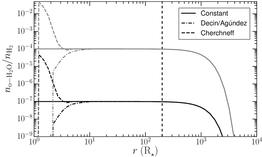
Figure 10: H₂O abundance profiles for three different chemical models at two different representative abundances at the radius indicated by the dashed vertical line: $n_{\mathrm{H}_{2}\mathrm{O}}/n_{\mathrm{H}_{2}}$ $=10^{-7}$ in black and $n_{\mathrm{H}_{2}\mathrm{O}}/n_{\mathrm{H}_{2}}$ $=10^{-4}$ in gray. The Constant abundance profile is a reference model. The Decin/Agúndez profile refers to the results of Decin et al. (2010a) and Agúndez et al. (2010). Cherchneff’s profile refers to her results of 2011. See Sect. 5.2.2 for further details.

In all three cases, the photodissociation radius is taken from the analytic formula of Groenewegen (1994). Which photodissociation radius is used here is not important since we want to gauge the sensitivity of H₂O/H₂O line-strength ratios to differences in the H₂O abundance profile caused by different formation mechanisms. Whatever the real photodissociation radius is, it should affect the presented models for different H₂O abundance profiles in the same way, and hence has no impact on our conclusions. As our interest lies in the inner and intermediate wind, we assume the same photodissociation law as from Groenewegen (1994) in the Decin et al. (2010a) and Agúndez et al. (2010) abundance profiles at radii beyond their maximal abundance value. In this way, we can compare the effects of the different formation mechanisms. To probe the effect of the absolute H₂O abundance, each of the profiles is scaled to a representative abundance at a radius in the outflow just before photodissociation sets in. In the model grid, this representative H₂O abundance scales from $10^{-7}$ up to $10^{-4}$ in factors of 10. The abundance profiles associated with the lowest and highest representative abundance are shown in Fig. 10. The higher representative abundances are not necessarily supported by the theories of Agúndez et al. (2010) and Cherchneff (2011). These abundance profiles are not tailored specifically according to the physical properties of the winds at different $\dot{M}_{\mathrm{g}}/\varv_{\infty\mathrm{,g}}$, and only provide an indication of how an inner- and intermediate-wind abundance gradient would affect the H₂O/H₂O line-strength ratios.

$\begin{array}[]{cc}\leavevmode\resizebox{256.0748pt}{}{\includegraphics{h2ograd_0v2_constant.pdf}}&\leavevmode\resizebox{256.0748pt}{}{\includegraphics{h2ograd_0v4_constant.pdf}}\\ \leavevmode\resizebox{256.0748pt}{}{\includegraphics{h2ograd_0v2_agundez.pdf}}&\leavevmode\resizebox{256.0748pt}{}{\includegraphics{h2ograd_0v4_agundez.pdf}}\\ \leavevmode\resizebox{256.0748pt}{}{\includegraphics{h2ograd_0v2_cherchneff.pdf}}&\leavevmode\resizebox{256.0748pt}{}{\includegraphics{h2ograd_0v4_cherchneff.pdf}}\end{array}$

Figure 11: H₂O/H₂O line-strength ratio versus the H₂O/CO line-strength ratio for a selection of H₂O transitions. The points with error bars give the measured line-strength ratios, color coded according to the $\dot{M}_{\mathrm{g}}/\varv_{\infty\mathrm{,g}}$ range to which the sources belong (in units of $\mathrm{M}_{\odot}\ \mathrm{yr}^{-1}\ \mathrm{km}^{-1}\ \mathrm{s}$), as indicated in the first panel. Undetected lines are not included in the figures. A black cross superimposed on the data point indicates that one of the H₂O lines is flagged as a blend. The colored curves show the predicted line-strength ratios for various values of $\dot{M}_{\mathrm{g}}/\varv_{\infty\mathrm{,g}}$, in the same range as the data points for each color. Each row of two panels shows results for different H₂O abundance profiles (see Sect. 5.2.2 for more details.) The crosses superimposed on the curves indicate the models for an increasing H₂O abundance from left to right in factors of 10, with the highest maximum value being $10^{-4}$. Adopted values for other parameters are listed in Table 5.

Two H₂O/H₂O line-strength ratios are shown in Fig. 11 for each of the H₂O abundance profiles. The first column compares the $J_{\mathrm{K}_{\mathrm{a}},\mathrm{K}_{\mathrm{c}}}=2_{2,1}-2_{1,2}$ line in the denominator to the $J_{\mathrm{K}_{\mathrm{a}},\mathrm{K}_{\mathrm{c}}}=2_{1,2}-1_{0,1}$ line in the numerator. The formation regions of these two lines differ slightly. The second column compares the $J_{\mathrm{K}_{\mathrm{a}},\mathrm{K}_{\mathrm{c}}}=3_{3,0}-2_{2,1}$ line in the denominator to the $J_{\mathrm{K}_{\mathrm{a}},\mathrm{K}_{\mathrm{c}}}=2_{1,2}-1_{0,1}$ line in the numerator, the former originating much deeper in the outflow than the latter. The H₂O/H₂O line-strength ratios are shown as a function of the H₂O/CO line-strength ratios on the horizontal axis for the H₂O line in common between both cases. The theoretical predictions are superimposed as full curves on the data points. The color coding is such that the same colors between data points and theoretical predictions have a similar $\dot{M}_{\mathrm{g}}/\varv_{\infty\mathrm{,g}}$ value. The points on the theoretical curves represent H₂O abundance values, increasing from left to right (as expected from the H₂O/CO line-strength ratio).

The major differences between the H₂O abundance profiles occur in the inner wind up to $r\sim 10$ R_⋆. We would expect to see the most profound effect on lines formed in the inner wind, but this is precisely where our line formation predictions are less reliable. That does not mean that lines formed primarily outside this zone remain unaffected. The nonlocal nature of radiative pumping implies that a high or low amount of H₂O in the inner wind can still affect emission lines formed further out owing to radiative pumping effects. Moreover, a different H₂O abundance profile may shift the line formation regions inward or outward in the wind. It is therefore worth checking how differences in the H₂O abundance profile in the intermediate as well as the inner wind affect the line strengths. Both columns in Fig. 11 compare the $J_{\mathrm{K}_{\mathrm{a}},\mathrm{K}_{\mathrm{c}}}=2_{1,2}-1_{0,1}$ line with a line that is formed deeper in the wind, but mostly at radii larger than $\sim 10$ R_⋆. All in all, the three abundance profiles predict subtle differences in line-strength ratios. We find that, in the case of optically thin lines (e.g., for $\dot{M}_{\mathrm{g}}/\varv_{\infty\mathrm{,g}}=3\times 10^{-8}$ $\mathrm{M}_{\odot}\ \mathrm{yr}^{-1}\ \mathrm{km}^{-1}\ \mathrm{s}$ and $\dot{M}_{\mathrm{g}}/\varv_{\infty\mathrm{,g}}=1\times 10^{-7}$ $\mathrm{M}_{\odot}\ \mathrm{yr}^{-1}\ \mathrm{km}^{-1}\ \mathrm{s}$, the black and blue curves in Fig. 11), the Decin/Agúndez H₂O abundance profile systematically increases the H₂O/H₂O line-strength ratios with respect to the constant abundance models. This should come as no surprise because the Decin/Agúndez H₂O abundance profile results in a lower abundance closer to the stellar surface, which in turn implies that the lines forming deeper in the wind decrease in strength relative to the lines forming further out. At high $\dot{M}_{\mathrm{g}}/\varv_{\infty\mathrm{,g}}$ the lines saturate and there is no noticeable difference between the constant and Decin/Agúndez cases. Compared to the constant abundance profile, the line strengths saturate more quickly for the Cherchneff abundance profile. When reaching representative abundances in the intermediate wind on the order of $10^{-4}$, there is no noticeable difference between different $\dot{M}_{\mathrm{g}}/\varv_{\infty\mathrm{,g}}$ values.

Comparing the predictions with the measurements, we are immediately confronted with the limitations of the PACS data, which have uncertainties that are too large to distinguish between the different abundance profiles. Nevertheless, the H₂O abundance is consistently predicted to be on the order of $10^{-6}-10^{-4}$ for the entire $\dot{M}_{\mathrm{g}}/\varv_{\infty\mathrm{,g}}$ range. This range is up to three orders of magnitude larger than what is predicted by Decin et al. (2010a) and Agúndez et al. (2010), as well as by Cherchneff (2011) for the case of CW Leo. The measurements for the H₂O/H₂O line-strength ratio involving the $J_{\mathrm{K}_{\mathrm{a}},\mathrm{K}_{\mathrm{c}}}=2_{2,1}-2_{1,2}$ line (first column in Fig. 11) tentatively suggest a trend where the ratio increases as $\dot{M}_{\mathrm{g}}/\varv_{\infty\mathrm{,g}}$ decreases (compare the green data points with the blue). Finally, our results for the Cherchneff abundance profile should not be taken at face value. While the profile for the low H₂O abundance value of $10^{-7}$ in the intermediate wind (as shown in Fig. 10) is representative of the chemical models calculated for CW Leo, the high abundance profiles are not. We artificially introduced extremely high abundance values in the inner wind (at $r<3\ \mathrm{R}_{\star}$) when scaling the profile up or down in representative intermediate-wind abundance. Of course, if we correct for such unreasonably high values, the H₂O abundance profile would flatten out and become more similar to the constant H₂O abundance profile. We included the experimental profiles to probe the effect of an increased inner-wind H₂O abundance on the H₂O/H₂O line-strength ratios. They do not represent a realistic view of what a chemical model following Cherchneff (2011) might look like if it was made to produce higher H₂O abundances.

It is clear that we have reached the limitations of a grid/sample-based approach. In-depth modeling of individual sources is required to rule out unique differences between observed sources and the model grid. This would allow us to derive further meaningful constraints on the H₂O abundance profile.

Table 6: Proposed H₂O formation mechanisms and the type of H₂O produced. Typical values for a set of stellar and circumstellar parameters are given: $\dot{M}_{\mathrm{g}}/\varv_{\infty\mathrm{,g}}$ the predicted H₂O abundance, radius $R_{\mathrm{i}}$ at which H₂O formation is expected to begin, radius $R_{\mathrm{o}}$ from which the H₂O abundance is expected to remain constant, a typical temperature range $T_{\mathrm{f}}$ for each mechanism, the original literature references (given below the table), and finally additional comments.

H2O formation mechanism	Type	$\dot{M}_{\mathrm{g}}/\varv_{\infty\mathrm{,g}}$	$n_{\mathrm{H}_{2}\mathrm{O}}/n_{\mathrm{H}_{2}}$	$R_{\star}$	$R_{\mathrm{i}}$	$R_{\mathrm{o}}$	Tf	Ref.	Comments
		($\frac{\mathrm{M}_{\odot}\ \mathrm{yr}^{-1}}{\mathrm{km}\ \mathrm{s}^{-1}}$)	(10-7)	($10^{13}$ cm)	(R⋆)	(R⋆)	(K)
Evaporation of icy bodies	cold	1.4-3.4$\times 10^{-6}$	4-24	7.65	15	/	$<500$	1,2,10	Ruled out
Radiative association H2 + O	cold	2.1$\times 10^{-6}$	1	6.5	150	750	$<200$	4,9	Ruled out
Fischer-Tropsch catalysis	intermediate	3.4$\times 10^{-6}$	1-100	7.0	15	45	$<500$	3	$\sim$ Fe-grain density
Shock chemistry	warm	1.0-4.0$\times 10^{-6}$	1-7	6.5	1.2	3.0	$>850$	7,8	$\sim$ shock strength
UV photodissociation	warm	1.4$\times 10^{-6}$	2	5.1	2	20	$>300$	5	$\sim$ degree of clumping
		6.7$\times 10^{-7}$	2	5.0	2	12	$>300$	6	$\sim$ degree of clumping
		6.7$\times 10^{-8}$	2	5.0	2	8	$>300$	6	$\sim$ degree of clumping
		6.7$\times 10^{-9}$	10	5.0	2	5	$>300$	6	$\sim$ degree of clumping

⁽¹⁾ Melnick et al. (2001), ⁽²⁾ Saavik Ford & Neufeld (2001), ⁽³⁾ Willacy (2004), ⁽⁴⁾ Agúndez & Cernicharo (2006), ⁽⁵⁾ Decin et al. (2010a), ⁽⁶⁾ Agúndez et al. (2010), ⁽⁷⁾ Cherchneff (2011), ⁽⁸⁾ Cherchneff (2012), ⁽⁹⁾ Talbi & Bacchus-Montabonel (2010), ⁽¹⁰⁾ Neufeld et al. (2011a).

6 Discussion

Different H₂O formation mechanisms lead to different properties of the H₂O abundance profile in the wind of carbon stars. In Table 6, we summarize these properties for five proposed mechanisms, although most of these predictions are model dependent and have been tailored to explain the H₂O observations of CW Leo, which is the prototypical high mass-loss rate carbon star. Hence a straightforward comparison of predicted values with the H₂O observations reported in this study is not feasible, unless the model assumptions of the H₂O formation mechanism agree with the properties of our sample stars. In the table we list the $\dot{M}_{\mathrm{g}}/\varv_{\infty\mathrm{,g}}$ value for which the H₂O abundance was derived and typical radii and temperatures associated with the formation mechanism. The mechanisms based on the evaporation of icy bodies and radiative association of H₂ and O are listed for completeness, but have been firmly ruled out as viable production mechanisms by previous studies (Neufeld et al. 2011a; Talbi & Bacchus-Montabonel 2010). That leaves one mechanism capable of producing cold H₂O in the intermediate wind from $\sim 15$ R_⋆ onward, and two mechanisms for producing warm H₂O in regions closer to the stellar surface. Our observations place four constraints on the H₂O formation mechanism.

1. As shown by previous studies for singular sources, and now confirmed to hold for all stars in a sample of 18 sources, H₂O exists in the inner and intermediate wind. For high mass-loss rate objects, we confirm the presence of H₂O at least as close to the stellar surface as $\sim$ 10 R_⋆, just outside the acceleration zone. For low mass-loss rate objects, H₂O is present around $\sim 2$ R_⋆.

2. The H₂O abundance is in the range of $10^{-6}-10^{-4}$. This is significantly higher than the predictions of state-of-the-art formation mechanisms.

3. The H₂O formation mechanism becomes less efficient with increasing mass-loss rate.

4. This negative correlation between H₂O abundance and mass-loss rate is observed for mass-loss rates higher than $\sim 5\times 10^{-7}\ \mathrm{M}_{\odot}\ \mathrm{yr}^{-1}$. The SRb sources in our sample do not follow the trend.

We now discuss properties of H₂O formation mechanisms that so far have not been disproved and relate them to the suggested criteria.

6.1 Fischer-Tropsch catalysis

Fischer-Tropsch catalysis allows for a broad range of H₂O abundances to be produced by tweaking the Fe-grain number density, but it is unclear how circumstellar column density affects the Fe-grain number density. However, in terms of the other requirements, the Fischer-Tropsch mechanism cannot be reconciled with our observations. Firstly, the presence of warm H₂O in the inner wind cannot be explained. Secondly, the mechanism would have to become more efficient at lower wind densities. This is counterintuitive for a mechanism based on dust grains acting as a catalyst because lower densities reduce the amount of interaction between dust and gas that is needed to produce H₂O. Thirdly, the mechanism cannot explain the presence of H₂O in SRb objects. In these sources, H₂O is located close to the stellar surface in too hot of an environment for the mechanism to operate. Even though Fischer-Tropsch catalysis may contribute to H₂O formation in carbon-rich environments, it seems very unlikely that it is universally active. Further modeling of this production mechanism for low mass-loss-rate objects needs to be performed to see if it still functions in low-density regions and whether or not it becomes more efficient.

6.2 UV photodissociation in the inner wind

Agúndez et al. (2010) have looked into a range of mass-loss rates for the mechanism of UV photodissociation, allowing a comparison with our results. Decin et al. (2010a) report results for the same mechanism for CW Leo. Table 6 summarizes the results for the different $\dot{M}_{\mathrm{g}}/\varv_{\infty\mathrm{,g}}$ values. In short, the photodissociation mechanism relies heavily on the degree of clumping in the wind for interstellar UV photons to be able to penetrate deeply into the wind. Therefore, the mechanism provides a natural way to explain a broad range of H₂O abundances.

The model results shown by Agúndez et al. (2010) also predict a decreasing H₂O abundance for objects with high mass-loss rates. This model predicts similar H₂O abundances for high and intermediate mass loss, but a sharp increase in H₂O abundance for low mass-loss rates. The discontinuity occurs when the major UV-shielded component, i.e., the clumps, becomes transparent. Our observations do not show such a sharp increase at a given mass-loss rate, but the model still provides enough flexibility in terms of the clump properties to allow for a more gradual dependence between the H₂O abundance and $\dot{M}_{\mathrm{g}}/\varv_{\infty\mathrm{,g}}$. Moreover, once both the UV-shielded and UV-exposed components become optically thin, the H₂O abundance can be expected to flatten off. This would explain why the SRb sources at $\dot{M}_{\mathrm{g}}<5\times 10^{-7}\ \mathrm{M}_{\odot}\ \mathrm{yr}^{-1}$ do not follow the negative correlation between the H₂O/CO line-strength ratio and the mass-loss rate. However, the H₂O abundance toward lower mass-loss rates does not flatten off, and instead decreases (as shown in Fig. 2). Hence, there appears to be a dependence on the stellar pulsation type, which is difficult to reconcile with this mechanism.

We cannot constrain the radial H₂O abundance gradient derived by Agúndez et al. (2010) given the uncertainties on the measured line strengths and the low sensitivity of the model predictions to density changes. Agúndez et al. also predict a maximum abundance of $2\times 10^{-7}$ to $10^{-6}$, depending on the mass-loss rate. However, we require these profiles to reach a maximum abundance up to three orders of magnitude greater, if they are to explain our H₂O/H₂O line-strength ratios. There might still be a reasonable degree of flexibility in the formalism to allow for this increase, but this would require further investigation.

The UV-photodissociation scenario suggests that the C¹⁷O and C¹⁸O isotopologues also provide atomic oxygen to produce the minor isotopologues H${}_{2}^{17}$O and H${}_{2}^{18}$O, while the main CO isotopologue shields itself from UV radiation. As a result, one expects an isotope-selective enhancement of the H${}_{2}^{17}$O and H${}_{2}^{18}$O abundances with respect to the main H₂O isotopologue. Recently, Neufeld et al. (2013) have shown for CW Leo that this isotope-selective enhancement is less than expected. They suggest that dissociation of C¹⁶O must contribute a significant number of oxygen atoms as well, if UV photodissociation serves as a basis for H₂O formation. Alternatively, if self-shielding of C¹⁶O proves to be too efficient, another mechanism that is indiscriminate of CO isotopologues, should contribute to H₂O formation in addition to UV photodissociation in the inner wind.

6.3 Shock-induced NLTE chemistry

As first proposed by Willacy & Cherchneff (1998) and Cherchneff (2006), shock-induced NLTE chemistry provides a universal method to produce H₂O in carbon-rich AGB stars: all of them show regular or semiregular pulsational variability, providing the shockwaves that are needed to break up CO and allow H₂O to form. H₂O is thus expected close to the stellar surface and a dependence on the variability type and pulsation amplitude could be explained in this framework. Important aspects of our H₂O analysis concern the similar H₂O line strengths between Miras and SRa sources, and the breakdown of the negative correlation between the H₂O/CO line-strength ratio and $\dot{M}_{\mathrm{g}}/\varv_{\infty\mathrm{,g}}$ at the low end of the range of mass-loss rate that is populated by SRb sources. It could be that SRa sources pulsate in a short-period fundamental mode and SRb sources in a first or second overtone mode. This could affect the shock strengths and densities, which in turn could influence H₂O formation. Indeed, Bowen (1988) found that the overtone pulsational modes experience smaller amplitude shocks. This could lead to a clear differentiation between Miras/SRa sources and SRb sources in terms of H₂O formation. Alternatively, the lesser regularity of the pulsations, a.k.a. periodicity, of SRb sources may also point to instabilities in multiple pulsation modes (e.g., Soszyński & Wood 2013), which could result in weaker shocks as well. In contrast, SRa sources are only unstable in one pulsation mode.

Because Cherchneff (2011, 2012) has focused on CW Leo, a source with a high mass-loss rate that has a period of 650 days, it is difficult to predict how her results would translate to the case of lower or multiple periods. Cherchneff (2012) states that similar trends can be expected in carbon-rich AGB stars other than CW Leo. She explains that a lower shock strength can result in a higher H₂O abundance due to the complex interplay between the consumption of free oxygen by both H₂O and SiO formation processes. As Cherchneff (2011, 2012) notes, these results rely heavily on the interplay between H₂O and SiO production, of which some involved reaction rates are not well constrained. If this process proves viable, it may explain why shorter-period pulsators, and thus lower shock strengths (Bowen 1988), show higher H₂O abundances. Even though they have a shorter pulsational period, SRb sources instead show lower H₂O abundances. However, they also pulsate less regularly. Cherchneff (2011, 2012) does not consider less regular shocks of lower strength, so it is unclear what their effect would be.

Cherchneff (2012) predicts a strong line variability with time for lines formed within $\sim 3$ R_⋆, i.e., where the shocks are strong. H₂O abundances can vary several orders of magnitude in this region, and for up to $\sim 80\%$ of one pulsational phase they are significantly higher than at larger distances from the stellar surface (see also Fig. 10). Outside this region, the H₂O abundance chemically freezes out to its final value over the course of one period, at $\sim 7\times 10^{-7}$. As shown in Sect. 5.2.2 for Mira and SRa sources, we require much larger abundances to explain the observed H₂O/H₂O line-strength ratios. Hence, the freeze-out over the course of one pulsation phase should occur at much larger abundances instead. It is at this point unclear whether that is possible in Cherchneff’s chemical model.

For SRb sources, we cannot draw any firm conclusions owing to the lower reliability of our models in the shocked region. The time variability for lines formed close to the stellar surface could provide an explanation for the erratic behavior of the H₂O/H₂O line-strength ratios observed in these sources.

Interestingly, a shock-induced formation mechanism would not discriminate between isotopologues when breaking up CO. As discussed before when considering H₂O formation by interstellar UV photodissociation, additional H₂O formation with ¹⁶O is needed (Neufeld et al. 2013). The shock mechanism readily provides this. Additionally, the shock mechanism and the UV photodissociation mechanism both predict significantly lower H₂O abundances than required. Therefore, our findings suggest that both mechanisms should contribute to warm H₂O formation in carbon-rich environments. Further studies expanding upon the parameter space of both chemical models are required to probe what range of H₂O abundances can be produced.

7 Conclusions

We report on new H₂O observations made with the PACS instrument onboard the Herschel space observatory for a sample of 18 carbon-rich AGB stars in the framework of the MESS guaranteed-time key project (P.I.: M. Groenewegen) and an OT2 project (P.I.: L. Decin). H₂O has been detected in all sample stars, spanning a broad range of mass-loss rates and several variability types. The H₂O emission lines include both warm and cold H₂O and trace the inner and intermediate wind, providing an unprecedented data set that contributes to solving the issue of H₂O formation in carbon-rich environments. We present line-strength measurements for CO, ¹³CO, ortho-H₂O, and para-H₂O between 60 $\mu$m and 190 $\mu$m.

For Miras and SRa sources, we find that the observed H₂O/CO line-strength ratios decrease as a function of the circumstellar density. A comparison of the CO line strengths with a model grid suggests that a single temperature power law with an exponent $\epsilon=0.4$ explains all CO observations with a moderate sensitivity to other parameters. As such, CO line measurements can be used as a reliable H₂ density tracer. We provide linear fitting coefficients for H₂O/CO line-strength ratios versus mass-loss rate, which can be used as either a distance-independent mass-loss indicator or to predict line-strength ratios if an estimate of the mass-loss rate is available.

A clear negative correlation is evident between the H₂O/CO line-strength ratios and the mass-loss rate for $\dot{M}_{\mathrm{g}}>5\times 10^{-7}\ \mathrm{M}_{\odot}\ \mathrm{yr}^{-1}$, regardless of the upper excitation level of the H₂O transitions or the variability type. The low mass-loss-rate SRb sources in our sample deviate from this trend. Only the gas terminal velocity and the dust-to-gas ratio noticeably impact the H₂O/CO line-strength ratios, but not enough to explain the negative correlation. This confirms that the H₂O/CO line-strength ratio is a valid distance-independent H₂O abundance tracer. As a result, the H₂O abundance needed to explain the observed line strengths depends on $\dot{M}_{\mathrm{g}}/\varv_{\infty\mathrm{,g}}$. When comparing H₂O/H₂O line-strength ratios with our model grid, we find that the measurements are not sensitive enough to distinguish between different H₂O abundance profiles.

Until now, five H₂O formation mechanisms have been suggested for carbon stars. Three of these mechanisms explain the presence of cold H₂O and two predict warm H₂O close to the stellar surface. Two cold-H₂O formation mechanisms have already been ruled out on the basis of previous studies. This leaves a H₂O formation mechanism based on Fischer-Tropsch catalysis on Fe grains in the intermediate wind, and two warm-H₂O formation mechanisms: one induced by pulsational shocks just outside the stellar surface, and one by photodissociation of molecules such as ¹³CO and SiO in the inner wind by interstellar UV photons. We derive four constraints that must be fulfilled by an H₂O formation mechanism: 1) warm H₂O is present close to or inside the acceleration zone in all 18 sources in our sample, 2) H₂O abundances are significantly higher than predicted by chemical formation mechanisms, 3) H₂O formation becomes less efficient with increasing mass loss regardless of the H₂O formation zone, and 4) the H₂O properties of the SRb sources are disparate from those of Miras and SRa sources.

The Fischer-Tropsch catalysis scenario fails to fully explain up to three of these criteria. Of the two warm-H₂O formation mechanisms, shock-induced NLTE chemistry looks the most promising, as the mechanism has the potential to fulfill all formation criteria. A mechanism based on interstellar UV photons cannot easily explain the peculiar behavior of the SRb sources in terms of H₂O emission, nor the absence of an isotope-selective enhancement of the H₂O isotopologues.

Both mechanisms currently fail to predict the high H₂O abundances required to reproduce the observed line strengths. This warrants further investigation of the chemical models.

Appendix A Radial profiles of 70-$\mu$m and 160-$\mu$m far-IR broadband emission

Figure 12 shows the radial profiles for two different carbon-rich AGB stars (see Table 7) observed with PACS at 70 $\mu$m. The top panel shows a point source, LL Peg, while the bottom panel shows an extended source, R Scl. In each figure the radial profile of Vesta, the PACS point spread function (PSF) calibration source, is also shown for comparison. For each object the full width at half maximum (FWHM) given in Table 7 is derived from a 2D-Gaussian fit to the bright, central object. The radial profiles are derived from aperture photometry using circular annuli up to 45”. The subtracted sky background is measured between annuli at 45 and 65”.

The FWHM at 70 $\mu$m is consistently $\sim$7-8” for eleven carbon-rich objects included in our sample. This is slightly larger than the $\sim$6” found for VESTA. Differences in, e.g., observing mode and data processing (HIPE photproject vs. scanamorphos) may underlie this small difference. The brightness of the central object and any extended emission also affect the Gaussian fit. Furthermore, particularly below 10% flux intensity levels the PSF deviates from a Gaussian shape showing a complicated tri-lobal PSF structure with diffraction spikes. At 160 $\mu$m the FHWM ranges from 12 to 14.5”, compared to the Vesta FWHM of 11.2”. At both wavelengths, RW LMi appears to be the most extended ’point’ source.

For the previously known extended sources R Scl and CW Leo we derive larger values for the Gaussian FWHM. However, these should not at all be taken to represent the observed shape for either R Scl (central point source with a small disk or shell; Maercker et al. 2012) or CW Leo (central, bright point source with a smooth wind and additional density enhancements; De Beck et al. 2012). For completeness, the FWHM values of these objects are included in Table 7 as well, but they are not included in the present study. PACS photometric data were not available for the objects in the sample not listed in Table 7. However, based on the data reduction of the spectroscopic data, these sources behave like a point source as well, similar to the sources listed here.

Table 7: In the sample for which PACS photometric data were available, we show FWHM of stars, as well as Vesta (PSF calibrator), R Scl, and CW Leo.

Star name	FWHM (″)
	70 $\mu$m	160 $\mu$m
RW Lmi	7.7	14.5
V Hya	7.0	13.2
II Lup	7.3	14.4
V Cyg	6.9	14.3
LL Peg	6.6	12.2
LP And	7.1	13.8
S Cep	7.1	12.7
Y CVn	6.7	12.1
R Lep	7.1	12.8
U Hya	7.1	13.1
W Ori	7.0	12.3
Vesta	5.6	11.2
R Scl	25.9	29.7
CW Leo	10.1	15.4

$\begin{array}[]{c}\leavevmode\resizebox{256.0748pt}{}{\includegraphics{radial_profiles_blue.pdf}}\\ \leavevmode\resizebox{256.0748pt}{}{\includegraphics{radial_profiles_red.pdf}}\end{array}$

Figure 12: The normalized flux as a function of the radial distance in arcseconds observed with PACS at 70 $\mu$m in the left panel, and at 160 $\mu$m in the right panel. Shown are Vesta (black dashed), LL Peg (blue), and R Scl (red).

Appendix B The PACS data

B.1 The spectra

Figures 13 through 24 show spectra of the sample sources observed in the framework of the MESS program. We subtracted the continuum of the spectra to improve readability (following Lombaert et al. 2013) and indicate the identified CO and H₂O emission lines. Other molecules are not included. The line strengths reported in Table. LABEL:table:intintmess have been measured before continuum subtraction was performed. Figures 26 up to 37 show the line scans of the sample sources observed in the framework of an OT2 program (P.I.: L. Decin). The six sources for which the line strengths are reported in Table LABEL:table:intintot2old were observed according to an old observation template, resulting in some overlapping wavelength regions between the line scans. For the next set of spectra, the observation scheme was optimized.

B.2 Integrated line strengths

Tables LABEL:table:intintmess, LABEL:table:intintot2old, and LABEL:table:intintot2new list the measured strengths of CO and H₂O lines in the MESS spectra, the extended setup of the OT2 line scans, and the optimized setup of the OT2 line scans, respectively. Other molecules have not been taken into account. See Sect. 2.3 for more details on the measurement process, and a few caveats. Finally, Tables LABEL:table:unidentified and LABEL:table:unidentified2 list the significantly detected emission lines in the OT2 data that are not attributed to CO or H₂O and for which we have not attempted to identify the molecular carrier.

$\begin{array}[]{cc}\leavevmode\resizebox{250.38434pt}{654.41338pt}{\includegraphics[angle={90}]{mess_rwlmi_B2A.pdf}}&\leavevmode\resizebox{250.38434pt}{654.41338pt}{\includegraphics[angle={90}]{mess_rwlmi_B2B.pdf}}\\ \end{array}$

Figure 13: Continuum-subtracted PACS spectrum of RW LMi is shown in black for the blue bands. The vertical lines indicate molecular identifications according to Table LABEL:table:intintmess: CO in red, ¹³CO in magenta, ortho-H₂O in green, and para-H₂O in cyan. If a black dashed line is superimposed over the identification line, the transition was not detected by our line-fitting algorithm. Lines have been indicated only if they occur in the wavelength ranges shared with the OT2 line scans (indicated in red in Table LABEL:table:intintmess) because the other identifications are less reliable (see Sect. 2.3). The PACS band is indicated in the upper left corner of each spectrum.

$\begin{array}[]{cc}\leavevmode\resizebox{250.38434pt}{682.86613pt}{\includegraphics[angle={90}]{mess_rwlmi_R1A.pdf}}&\leavevmode\resizebox{250.38434pt}{682.86613pt}{\includegraphics[angle={90}]{mess_rwlmi_R1B.pdf}}\\ \end{array}$

Figure 14: Continuum-subtracted PACS spectrum of RW LMi is shown for the red bands. The line types are the same as Fig. 13.

$\begin{array}[]{cc}\leavevmode\resizebox{250.38434pt}{682.86613pt}{\includegraphics[angle={90}]{mess_vhya_B2A.pdf}}&\leavevmode\resizebox{250.38434pt}{682.86613pt}{\includegraphics[angle={90}]{mess_vhya_B2B.pdf}}\\ \end{array}$

Figure 15: Continuum-subtracted PACS spectrum of V Hya is shown for the blue bands. The line types are the same as Fig. 13.

$\begin{array}[]{cc}\leavevmode\resizebox{250.38434pt}{682.86613pt}{\includegraphics[angle={90}]{mess_vhya_R1A.pdf}}&\leavevmode\resizebox{250.38434pt}{682.86613pt}{\includegraphics[angle={90}]{mess_vhya_R1B.pdf}}\\ \end{array}$

Figure 16: Continuum-subtracted PACS spectrum of V Hya is shown for the red bands. The line types are the same as Fig. 13.

$\begin{array}[]{cc}\leavevmode\resizebox{250.38434pt}{682.86613pt}{\includegraphics[angle={90}]{mess_iilup_B2A.pdf}}&\leavevmode\resizebox{250.38434pt}{682.86613pt}{\includegraphics[angle={90}]{mess_iilup_B2B.pdf}}\\ \end{array}$

Figure 17: Continuum-subtracted PACS spectrum of II Lup is shown for the blue bands. The line types are the same as Fig. 13.

$\begin{array}[]{cc}\leavevmode\resizebox{250.38434pt}{682.86613pt}{\includegraphics[angle={90}]{mess_iilup_R1A.pdf}}&\leavevmode\resizebox{250.38434pt}{682.86613pt}{\includegraphics[angle={90}]{mess_iilup_R1B.pdf}}\\ \end{array}$

Figure 18: Continuum-subtracted PACS spectrum of II Lup is shown for the red bands. The line types are the same as Fig. 13.

$\begin{array}[]{cc}\leavevmode\resizebox{250.38434pt}{682.86613pt}{\includegraphics[angle={90}]{mess_vcyg_B2A.pdf}}&\leavevmode\resizebox{250.38434pt}{682.86613pt}{\includegraphics[angle={90}]{mess_vcyg_B2B.pdf}}\\ \end{array}$

Figure 19: Continuum-subtracted PACS spectrum of V Cyg is shown for the blue bands. The line types are the same as Fig. 13.

$\begin{array}[]{cc}\leavevmode\resizebox{250.38434pt}{682.86613pt}{\includegraphics[angle={90}]{mess_vcyg_R1A.pdf}}&\leavevmode\resizebox{250.38434pt}{682.86613pt}{\includegraphics[angle={90}]{mess_vcyg_R1B.pdf}}\\ \end{array}$

Figure 20: Continuum-subtracted PACS spectrum of V Cyg is shown for the red bands. The line types are the same as Fig. 13.

$\begin{array}[]{cc}\leavevmode\resizebox{250.38434pt}{682.86613pt}{\includegraphics[angle={90}]{mess_llpeg_B2A.pdf}}&\leavevmode\resizebox{250.38434pt}{682.86613pt}{\includegraphics[angle={90}]{mess_llpeg_B2B.pdf}}\\ \end{array}$

Figure 21: Continuum-subtracted PACS spectrum of LL Peg is shown for the blue bands. The line types are the same as Fig. 13.

$\begin{array}[]{cc}\leavevmode\resizebox{250.38434pt}{682.86613pt}{\includegraphics[angle={90}]{mess_llpeg_R1A.pdf}}&\leavevmode\resizebox{250.38434pt}{682.86613pt}{\includegraphics[angle={90}]{mess_llpeg_R1B.pdf}}\\ \end{array}$

Figure 22: Continuum-subtracted PACS spectrum of LL Peg is shown for the red bands. The line types are the same as Fig. 13.

$\begin{array}[]{cc}\leavevmode\resizebox{250.38434pt}{682.86613pt}{\includegraphics[angle={90}]{mess_lpand_B2A.pdf}}&\leavevmode\resizebox{250.38434pt}{682.86613pt}{\includegraphics[angle={90}]{mess_lpand_B2B.pdf}}\\ \end{array}$

Figure 23: Continuum-subtracted PACS spectrum of LP And is shown for the blue bands. The line types are the same as Fig. 13.

$\begin{array}[]{cc}\leavevmode\resizebox{250.38434pt}{682.86613pt}{\includegraphics[angle={90}]{mess_lpand_R1A.pdf}}&\leavevmode\resizebox{250.38434pt}{682.86613pt}{\includegraphics[angle={90}]{mess_lpand_R1B.pdf}}\\ \end{array}$

Figure 24: Continuum-subtracted PACS spectrum of LP And is shown for the red bands. The line types are the same as Fig. 13.

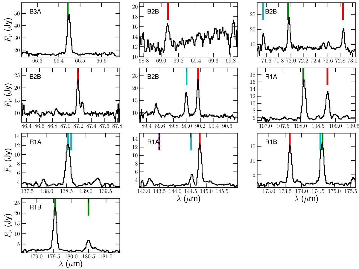
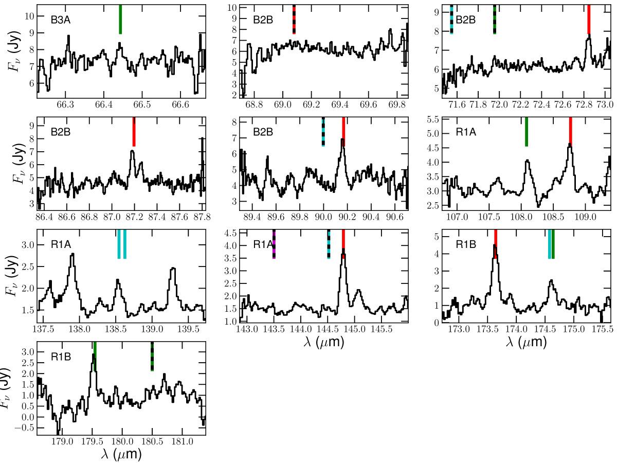
Figure 27: Line scans of R Lep. The line types are the same as Fig. 26.

Figure 28: Line scans of W Ori. The line types are the same as Fig. 26.

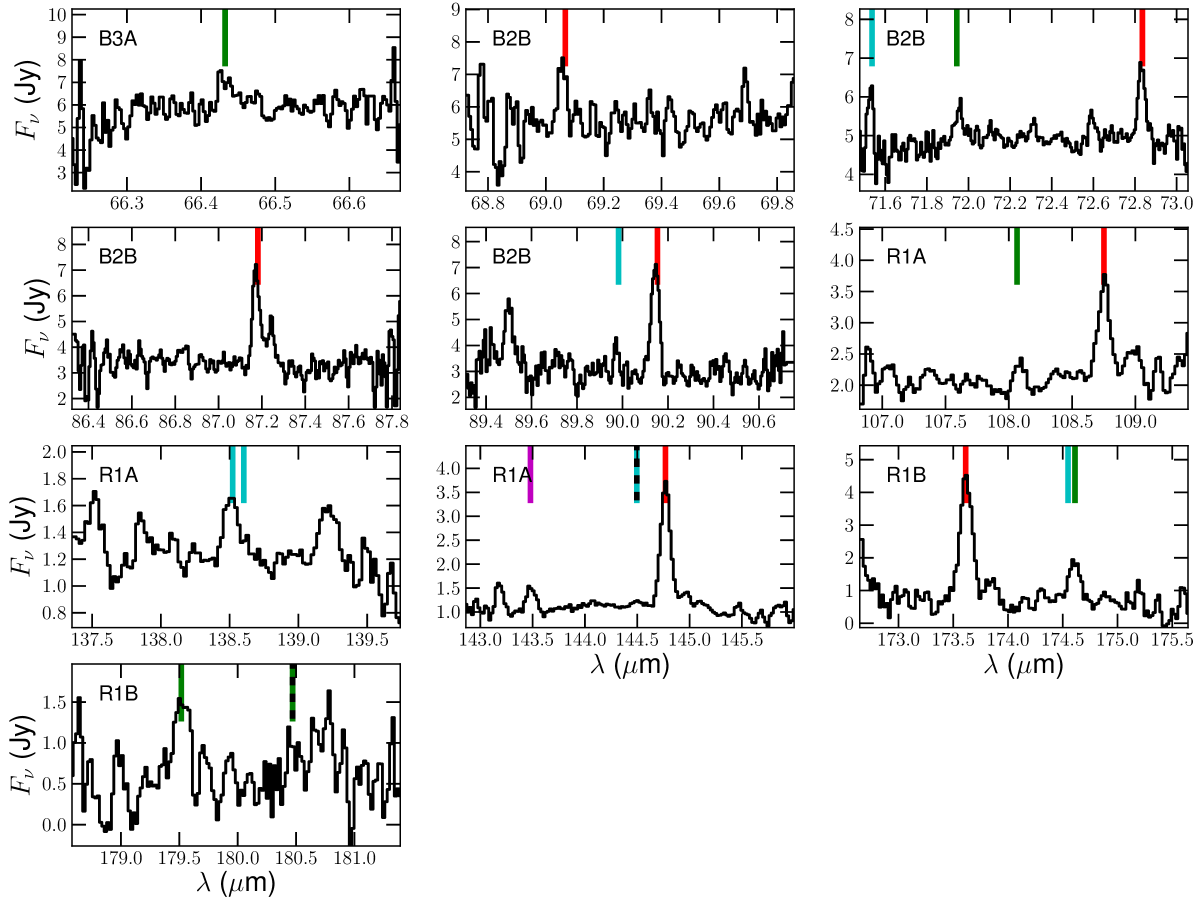
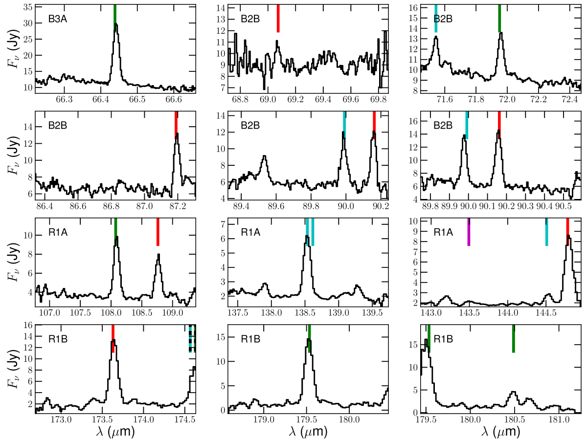
Figure 29: Line scans of U Hya. The line types are the same as Fig. 26.

Figure 30: Line scans of QZ Mus. The line types are the same as Fig. 26.

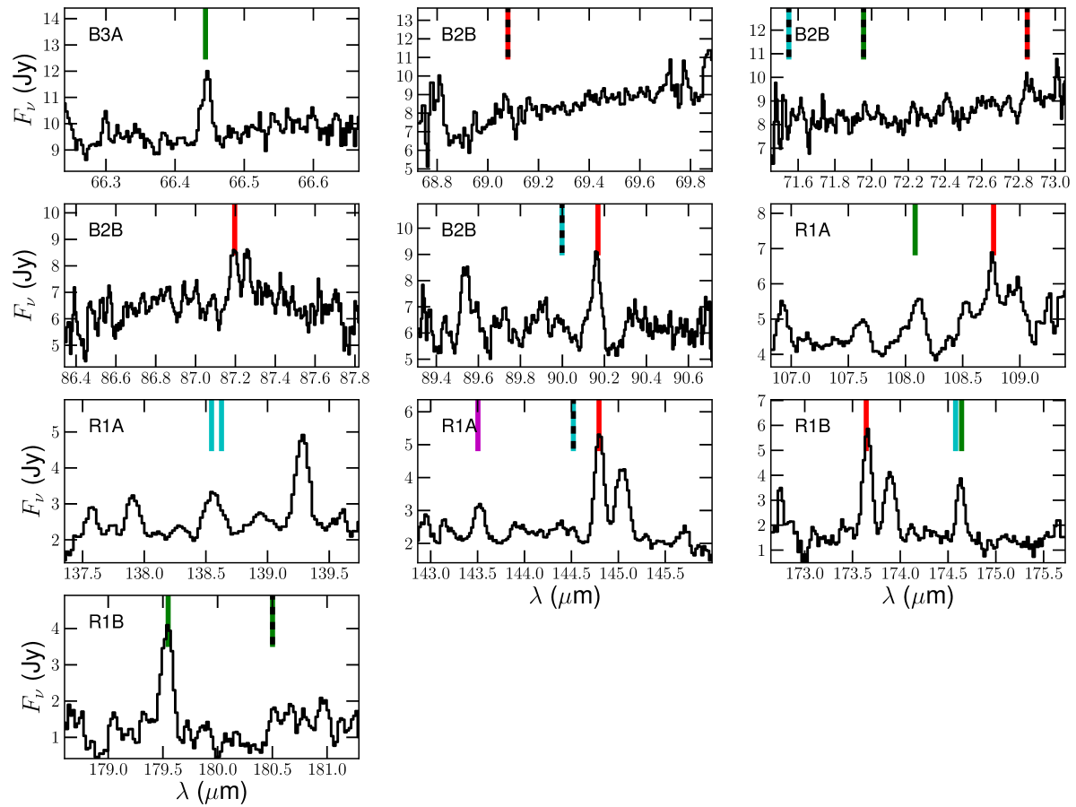
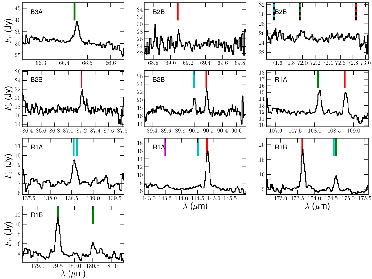
Figure 31: Line scans of Y CVn. The line types are the same as Fig. 26.

Figure 32: Line scans of AFGL 4202. The line types are the same as Fig. 26.

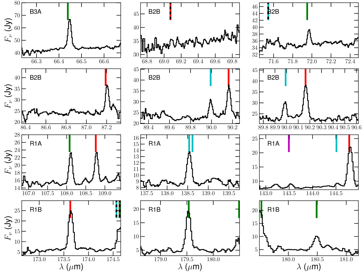
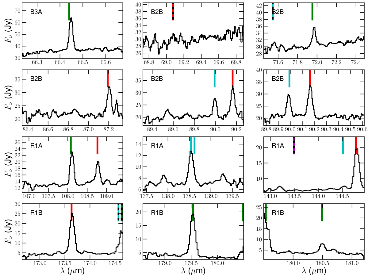
Figure 33: Line scans of V821 Her. The line types are the same as Fig. 26.

Figure 34: Line scans of V1417 Aql. The line types are the same as Fig. 26.

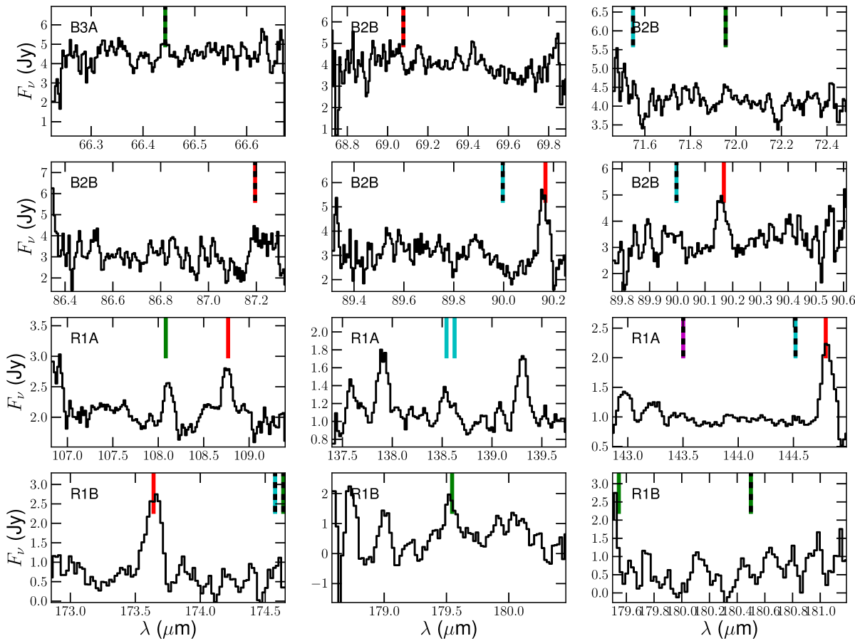
Figure 35: Line scans of S Cep. The line types are the same as Fig. 26.

Figure 36: Line scans of RV Cyg. The line types are the same as Fig. 26.

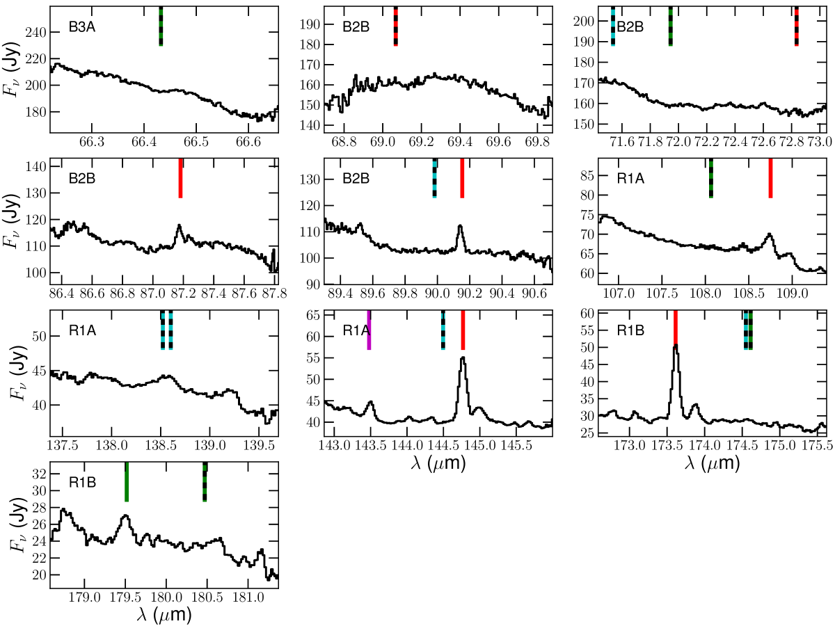
Figure 37: Line scans of LL Peg. The line types are the same as Fig. 26.

Table 8: Integrated line strengths $I_{\mathrm{int}}$ (W m^-2) for a selection of lines in the PACS spectra of carbon stars in the MESS sample. The rest wavelength $\lambda_{0}$ ($\mu$m) of the transition is indicated. The percentages between brackets give the uncertainty on $I_{\mathrm{int}}$, which includes both the fitting uncertainty and the PACS absolute-flux-calibration uncertainty of 20%. Line strengths indicated with $\star$ are flagged for potential line blends. Transitions that might cause the line blend are mentioned immediately below the flagged transition. Molecular transitions indicated in red coincide with the wavelength range of the line scans in the OT2 program. These detections are not expected to be affected by blends with molecules other than CO and H₂O. Detections listed in black have to be treated with caution, as they have not been checked for potential blending with other molecules.

				RW LMi	V Hya	II Lup	V Cyg	LL Peg	LP And
PACS	Molecule	Rotational	$\lambda_{0}$	$I_{\mathrm{int}}$
band		transition	$\mu$m	(W m-2)
R1B	p-H2O	$J_{\mathrm{K}_{\mathrm{a}},\mathrm{K}_{\mathrm{c}}}=4_{1,3}-4_{0,4}$	187.11	/	⋆ 7.71e-17 (26.2%)	5.83e-17 (30.5%)	/	/	4.23e-17 (25.0%)
	CO	$J=14-13$	186.00	9.19e-16 (20.3%)	4.61e-16 (20.2%)	4.57e-16 (20.4%)	1.98e-16 (21.7%)	2.29e-16 (21.1%)	2.64e-16 (20.7%)
	13CO	$J=15-14$	181.61	6.11e-17 (26.1%)	/	1.28e-16 (21.9%)	/	5.41e-17 (28.8%)	/
	o-H2O	$J_{\mathrm{K}_{\mathrm{a}},\mathrm{K}_{\mathrm{c}}}=2_{2,1}-2_{1,2}$	180.49	1.43e-16 (24.6%)	⋆ 9.43e-17 (24.5%)	4.73e-17 (33.4%)	/	/	5.84e-17 (25.8%)
	o-H2O	$J_{\mathrm{K}_{\mathrm{a}},\mathrm{K}_{\mathrm{c}}}=2_{1,2}-1_{0,1}$	179.53	4.47e-16 (20.5%)	2.98e-16 (20.3%)	1.62e-16 (21.6%)	1.72e-16 (20.9%)	/	1.25e-16 (21.7%)
	o-H2O	$J_{\mathrm{K}_{\mathrm{a}},\mathrm{K}_{\mathrm{c}}}=3_{0,3}-2_{1,2}$	174.63	⋆ 3.01e-16 (22.0%)	⋆ 1.86e-16 (21.1%)	⋆ 1.08e-16 (24.1%)	⋆ 8.27e-17 (23.6%)	/	⋆ 5.49e-17 (26.9%)
	p-H2O	$J_{\mathrm{K}_{\mathrm{a}},\mathrm{K}_{\mathrm{c}}}=5_{3,3}-6_{0,6}$	174.61	Blended	Blended	Blended	Blended	/	Blended
	CO	$J=15-14$	173.63	9.88e-16 (20.2%)	6.10e-16 (20.1%)	5.12e-16 (20.2%)	2.21e-16 (20.4%)	2.56e-16 (20.8%)	3.45e-16 (20.3%)
	13CO	$J=16-15$	170.29	1.01e-16 (28.2%)	/	9.28e-17 (24.8%)	⋆ 1.81e-17 (48.5%)	4.60e-17 (29.4%)	⋆ 6.49e-17 (24.5%)
	p-H2O	$J_{\mathrm{K}_{\mathrm{a}},\mathrm{K}_{\mathrm{c}}}=6_{3,3}-6_{2,4}$	170.14	/	/	/	Blended	/	/
	CO	$J=16-15$	162.81	1.05e-15 (20.1%)	6.35e-16 (20.1%)	5.45e-16 (20.3%)	3.22e-16 (20.3%)	2.83e-16 (20.6%)	3.42e-16 (20.1%)
	o-H2O	$J_{\mathrm{K}_{\mathrm{a}},\mathrm{K}_{\mathrm{c}}}=5_{3,2}-5_{2,3}$	160.51	2.65e-16 (21.3%)	1.20e-16 (23.4%)	1.20e-16 (23.4%)	/	9.01e-17 (25.3%)	1.17e-16 (21.5%)
	13CO	$J=17-16$	160.30	1.36e-16 (24.0%)	/	1.89e-16 (21.6%)	/	1.04e-16 (24.4%)	6.79e-17 (22.8%)
	o-H2O	$J_{\mathrm{K}_{\mathrm{a}},\mathrm{K}_{\mathrm{c}}}=8_{4,5}-7_{5,2}$	159.05	⋆ 6.87e-17 (29.5%)	/	2.24e-17 (37.1%)	/	/	/
	o-H2O	$J_{\mathrm{K}_{\mathrm{a}},\mathrm{K}_{\mathrm{c}}}=5_{2,3}-4_{3,2}$	156.27	⋆ 2.95e-16 (20.8%)	⋆ 9.70e-17 (22.0%)	⋆ 6.93e-17 (25.5%)	⋆ 7.01e-17 (28.9%)	/	⋆ 5.49e-17 (28.8%)
	p-H2O	$J_{\mathrm{K}_{\mathrm{a}},\mathrm{K}_{\mathrm{c}}}=3_{2,2}-3_{1,3}$	156.19	Blended	Blended	Blended	Blended	/	Blended
	CO	$J=17-16$	153.27	1.30e-15 (20.2%)	7.15e-16 (20.1%)	5.61e-16 (20.4%)	2.90e-16 (20.3%)	3.51e-16 (20.7%)	4.55e-16 (20.3%)
	13CO	$J=18-17$	151.43	2.23e-16 (23.1%)	4.84e-17 (27.9%)	1.24e-16 (22.7%)	⋆ 5.95e-17 (28.7%)	3.61e-17 (40.8%)	⋆ 5.68e-17 (31.6%)
	p-H2O	$J_{\mathrm{K}_{\mathrm{a}},\mathrm{K}_{\mathrm{c}}}=4_{3,1}-4_{2,2}$	146.92	9.49e-17 (27.0%)	2.87e-17 (32.7%)	/	/	⋆ 5.42e-17 (34.3%)	/
	CO	$J=18-17$	144.78	1.07e-15 (20.4%)	5.83e-16 (20.2%)	4.27e-16 (20.4%)	3.07e-16 (20.3%)	2.73e-16 (21.5%)	3.67e-16 (20.2%)
	13CO	$J=19-18$	143.49	/	/	1.08e-16 (21.9%)	/	/	4.72e-17 (26.2%)
R1A	CO	$J=18-17$	144.78	9.84e-16 (20.4%)	5.52e-16 (20.1%)	4.59e-16 (20.3%)	2.66e-16 (20.6%)	2.53e-16 (20.5%)	3.56e-16 (20.2%)
	13CO	$J=19-18$	143.49	/	/	1.19e-16 (21.3%)	/	/	2.62e-17 (36.1%)
	p-H2O	$J_{\mathrm{K}_{\mathrm{a}},\mathrm{K}_{\mathrm{c}}}=8_{4,4}-7_{5,3}$	138.64	⋆ 2.58e-16 (22.0%)	⋆ 1.74e-16 (21.0%)	⋆ 9.89e-17 (25.9%)	⋆ 1.14e-16 (22.9%)	/	⋆ 5.62e-17 (27.7%)
	p-H2O	$J_{\mathrm{K}_{\mathrm{a}},\mathrm{K}_{\mathrm{c}}}=3_{1,3}-2_{0,2}$	138.53	Blended	Blended	Blended	Blended	/	Blended
	CO	$J=19-18$	137.20	9.56e-16 (20.1%)	5.64e-16 (20.1%)	3.97e-16 (20.4%)	2.91e-16 (20.4%)	2.83e-16 (20.7%)	3.22e-16 (20.2%)
	o-H2O	$J_{\mathrm{K}_{\mathrm{a}},\mathrm{K}_{\mathrm{c}}}=3_{3,0}-3_{2,1}$	136.50	⋆ 2.44e-16 (27.8%)	⋆ 5.84e-17 (43.2%)	3.45e-17 (36.8%)	⋆ 6.86e-17 (30.3%)	/	3.53e-17 (44.0%)
	13CO	$J=20-19$	136.35	2.02e-16 (26.2%)	Blended	1.45e-16 (22.2%)	2.12e-17 (43.6%)	/	5.50e-17 (32.5%)
	o-H2O	$J_{\mathrm{K}_{\mathrm{a}},\mathrm{K}_{\mathrm{c}}}=5_{1,4}-5_{0,5}$	134.94	3.36e-16 (21.5%)	1.78e-16 (21.1%)	1.18e-16 (23.3%)	5.50e-17 (29.2%)	6.48e-17 (30.9%)	9.22e-17 (23.2%)
	o-H2O	$J_{\mathrm{K}_{\mathrm{a}},\mathrm{K}_{\mathrm{c}}}=4_{2,3}-4_{1,4}$	132.41	⋆ 2.22e-16 (27.4%)	9.81e-17 (25.2%)	/	/	/	/
	CO	$J=20-19$	130.37	⋆ 1.64e-15 (20.1%)	⋆ 9.09e-16 (20.1%)	⋆ 6.55e-16 (20.2%)	⋆ 4.29e-16 (20.3%)	⋆ 4.19e-16 (20.4%)	⋆ 5.89e-16 (20.1%)
	p-H2O	$J_{\mathrm{K}_{\mathrm{a}},\mathrm{K}_{\mathrm{c}}}=7_{5,3}-8_{2,6}$	130.32	Blended	Blended	Blended	Blended	Blended	Blended
	13CO	$J=21-20$	129.89	3.00e-16 (23.6%)	1.35e-16 (23.8%)	1.93e-16 (21.9%)	/	1.12e-16 (24.4%)	1.50e-16 (21.0%)
	p-H2O	$J_{\mathrm{K}_{\mathrm{a}},\mathrm{K}_{\mathrm{c}}}=4_{0,4}-3_{1,3}$	125.35	2.84e-16 (23.7%)	1.27e-16 (25.2%)	⋆ 9.16e-17 (31.3%)	5.07e-17 (28.5%)	/	⋆ 9.55e-17 (25.2%)
	CO	$J=21-20$	124.19	1.02e-15 (20.3%)	6.02e-16 (20.3%)	3.96e-16 (20.5%)	2.56e-16 (20.6%)	2.16e-16 (22.0%)	4.07e-16 (20.3%)
	13CO	$J=22-21$	124.02	/	/	1.12e-16 (25.8%)	/	/	2.15e-17 (46.6%)
	o-H2O	$J_{\mathrm{K}_{\mathrm{a}},\mathrm{K}_{\mathrm{c}}}=4_{3,2}-4_{2,3}$	121.72	/	/	/	/	/	⋆ 4.94e-17 (29.6%)
	13CO	$J=23-22$	118.66	⋆ 1.12e-15 (20.9%)	⋆ 6.17e-16 (20.3%)	⋆ 4.57e-16 (21.2%)	⋆ 2.65e-16 (21.0%)	⋆ 2.65e-16 (20.9%)	⋆ 3.71e-16 (20.5%)
	CO	$J=22-21$	118.58	Blended	Blended	Blended	Blended	Blended	Blended
	o-H2O	$J_{\mathrm{K}_{\mathrm{a}},\mathrm{K}_{\mathrm{c}}}=7_{3,4}-6_{4,3}$	116.78	/	⋆ 9.63e-17 (28.2%)	5.66e-17 (37.2%)	3.14e-17 (51.1%)	⋆ 1.13e-16 (27.0%)	⋆ 1.00e-16 (24.0%)
	p-H2O	$J_{\mathrm{K}_{\mathrm{a}},\mathrm{K}_{\mathrm{c}}}=5_{3,3}-5_{2,4}$	113.95	/	/	⋆ 1.26e-16 (35.5%)	/	/	4.49e-17 (31.4%)
	13CO	$J=24-23$	113.75	/	/	5.40e-17 (36.1%)	/	/	3.83e-17 (29.0%)
	o-H2O	$J_{\mathrm{K}_{\mathrm{a}},\mathrm{K}_{\mathrm{c}}}=4_{1,4}-3_{0,3}$	113.54	⋆ 1.49e-15 (20.3%)	⋆ 8.92e-16 (20.2%)	⋆ 4.79e-16 (20.5%)	⋆ 4.48e-16 (20.6%)	⋆ 2.64e-16 (21.7%)	⋆ 4.35e-16 (20.2%)
	CO	$J=23-22$	113.46	Blended	Blended	Blended	Blended	Blended	Blended
	o-H2O	$J_{\mathrm{K}_{\mathrm{a}},\mathrm{K}_{\mathrm{c}}}=7_{4,3}-7_{3,4}$	112.51	1.30e-16 (47.6%)	/	⋆ 1.49e-16 (53.7%)	/	⋆ 1.27e-16 (35.2%)	/
	CO	$J=24-23$	108.76	1.03e-15 (20.9%)	5.71e-16 (20.5%)	3.24e-16 (21.7%)	2.00e-16 (21.7%)	1.96e-16 (23.9%)	3.42e-16 (20.6%)
	o-H2O	$J_{\mathrm{K}_{\mathrm{a}},\mathrm{K}_{\mathrm{c}}}=2_{2,1}-1_{1,0}$	108.07	6.63e-16 (21.6%)	2.84e-16 (21.7%)	1.74e-16 (24.8%)	1.73e-16 (23.4%)	/	8.01e-17 (27.9%)
	13CO	$J=26-25$	105.06	/	/	/	/	/	4.41e-17 (34.0%)
	CO	$J=25-24$	104.44	9.97e-16 (21.5%)	⋆ 6.75e-16 (20.4%)	3.36e-16 (22.2%)	2.79e-16 (22.5%)	1.77e-16 (30.4%)	3.38e-16 (20.8%)
B2B	CO	$J=27-26$	96.77	5.41e-16 (20.8%)	⋆ 4.00e-16 (21.5%)	⋆ 2.44e-16 (23.5%)	1.67e-16 (25.9%)	8.39e-17 (38.9%)	1.82e-16 (21.7%)
	p-H2O	$J_{\mathrm{K}_{\mathrm{a}},\mathrm{K}_{\mathrm{c}}}=5_{1,5}-4_{0,4}$	95.63	2.82e-16 (24.0%)	1.13e-16 (24.5%)	5.61e-17 (54.8%)	/	/	/
	o-H2O	$J_{\mathrm{K}_{\mathrm{a}},\mathrm{K}_{\mathrm{c}}}=4_{4,1}-4_{3,2}$	94.71	9.47e-17 (38.0%)	/	/	/	/	/
	o-H2O	$J_{\mathrm{K}_{\mathrm{a}},\mathrm{K}_{\mathrm{c}}}=6_{2,5}-6_{1,6}$	94.64	1.60e-16 (29.2%)	6.74e-17 (29.3%)	/	/	/	/
	p-H2O	$J_{\mathrm{K}_{\mathrm{a}},\mathrm{K}_{\mathrm{c}}}=7_{3,5}-7_{2,6}$	93.38	⋆ 7.03e-16 (21.1%)	⋆ 4.98e-16 (20.7%)	⋆ 2.61e-16 (22.1%)	⋆ 1.42e-16 (23.0%)	⋆ 1.21e-16 (25.7%)	⋆ 2.70e-16 (20.5%)
	CO	$J=28-27$	93.35	Blended	Blended	Blended	Blended	Blended	Blended
	13CO	$J=30-29$	91.18	⋆ 1.64e-16 (24.9%)	/	⋆ 8.52e-17 (37.7%)	/	/	5.15e-17 (28.6%)
	CO	$J=29-28$	90.16	1.01e-15 (20.6%)	⋆ 5.17e-16 (20.4%)	2.11e-16 (22.2%)	2.14e-16 (21.2%)	⋆ 2.31e-16 (23.8%)	2.89e-16 (20.9%)
	p-H2O	$J_{\mathrm{K}_{\mathrm{a}},\mathrm{K}_{\mathrm{c}}}=3_{2,2}-2_{1,1}$	89.99	3.71e-16 (24.1%)	1.17e-16 (24.1%)	5.49e-17 (41.3%)	5.09e-17 (40.6%)	9.45e-17 (33.4%)	5.53e-17 (37.3%)
	13CO	$J=31-30$	88.27	/	/	6.66e-17 (29.5%)	/	/	/
	CO	$J=30-29$	87.19	8.55e-16 (20.4%)	4.76e-16 (20.5%)	1.75e-16 (24.9%)	1.24e-16 (26.1%)	/	⋆ 3.45e-16 (20.6%)
	o-H2O	$J_{\mathrm{K}_{\mathrm{a}},\mathrm{K}_{\mathrm{c}}}=7_{1,6}-7_{0,7}$	84.77	/	/	6.22e-17 (36.2%)	/	/	/
	CO	$J=31-30$	84.41	⋆ 8.60e-16 (20.6%)	⋆ 4.55e-16 (20.7%)	⋆ 2.12e-16 (24.2%)	1.82e-16 (25.3%)	/	2.55e-16 (21.1%)
	p-H2O	$J_{\mathrm{K}_{\mathrm{a}},\mathrm{K}_{\mathrm{c}}}=6_{0,6}-5_{1,5}$	83.28	⋆ 2.13e-16 (32.1%)	1.14e-16 (22.5%)	/	/	/	/
	13CO	$J=33-32$	82.99	/	/	/	/	/	⋆ 3.62e-17 (39.9%)
	o-H2O	$J_{\mathrm{K}_{\mathrm{a}},\mathrm{K}_{\mathrm{c}}}=8_{3,6}-8_{2,7}$	82.98	/	/	/	/	/	Blended
	o-H2O	$J_{\mathrm{K}_{\mathrm{a}},\mathrm{K}_{\mathrm{c}}}=6_{1,6}-5_{0,5}$	82.03	4.06e-16 (21.7%)	⋆ 2.91e-16 (20.8%)	⋆ 1.84e-16 (25.7%)	1.25e-16 (27.1%)	/	⋆ 7.73e-17 (26.0%)
	CO	$J=32-31$	81.81	4.94e-16 (21.0%)	3.55e-16 (20.5%)	8.47e-17 (27.0%)	1.12e-16 (27.8%)	/	2.07e-16 (20.8%)
	p-H2O	$J_{\mathrm{K}_{\mathrm{a}},\mathrm{K}_{\mathrm{c}}}=8_{3,5}-7_{4,4}$	81.69	/	/	/	/	/	5.02e-17 (28.3%)
	p-H2O	$J_{\mathrm{K}_{\mathrm{a}},\mathrm{K}_{\mathrm{c}}}=7_{2,6}-7_{1,7}$	81.22	7.07e-17 (39.8%)	/	/	/	/	/
	CO	$J=33-32$	79.36	5.52e-16 (21.1%)	⋆ 4.83e-16 (20.7%)	1.65e-16 (28.1%)	8.18e-17 (33.3%)	/	2.20e-16 (21.8%)
	p-H2O	$J_{\mathrm{K}_{\mathrm{a}},\mathrm{K}_{\mathrm{c}}}=6_{1,5}-5_{2,4}$	78.93	⋆ 3.45e-16 (27.0%)	/	/	/	/	⋆ 1.22e-16 (28.4%)
	o-H2O	$J_{\mathrm{K}_{\mathrm{a}},\mathrm{K}_{\mathrm{c}}}=4_{2,3}-3_{1,2}$	78.74	6.37e-16 (20.7%)	3.23e-16 (21.3%)	1.25e-16 (31.3%)	1.84e-16 (23.6%)	/	1.53e-16 (23.6%)
	o-H2O	$J_{\mathrm{K}_{\mathrm{a}},\mathrm{K}_{\mathrm{c}}}=7_{5,2}-7_{4,3}$	77.76	4.78e-17 (33.5%)	/	/	/	/	/
	CO	$J=34-33$	77.06	⋆ 5.89e-16 (21.8%)	⋆ 4.48e-16 (20.6%)	8.66e-17 (29.4%)	⋆ 1.15e-16 (25.6%)	8.88e-17 (31.6%)	1.76e-16 (21.6%)
	13CO	$J=36-35$	76.17	/	/	⋆ 9.11e-17 (30.8%)	/	/	/
	o-H2O	$J_{\mathrm{K}_{\mathrm{a}},\mathrm{K}_{\mathrm{c}}}=5_{5,0}-5_{4,1}$	75.91	/	/	5.54e-17 (36.7%)	/	/	/
	o-H2O	$J_{\mathrm{K}_{\mathrm{a}},\mathrm{K}_{\mathrm{c}}}=6_{5,2}-6_{4,3}$	75.83	/	/	⋆ 1.72e-17 (89.9%)	/	/	/
	p-H2O	$J_{\mathrm{K}_{\mathrm{a}},\mathrm{K}_{\mathrm{c}}}=7_{5,3}-7_{4,4}$	75.81	⋆ 2.24e-16 (25.9%)	/	Blended	/	/	⋆ 1.58e-16 (22.6%)
	p-H2O	$J_{\mathrm{K}_{\mathrm{a}},\mathrm{K}_{\mathrm{c}}}=5_{5,1}-5_{4,2}$	75.78	Blended	/	⋆ 1.19e-16 (34.8%)	/	/	Blended
	o-H2O	$J_{\mathrm{K}_{\mathrm{a}},\mathrm{K}_{\mathrm{c}}}=3_{2,1}-2_{1,2}$	75.38	7.81e-16 (20.6%)	4.47e-16 (20.4%)	2.33e-16 (21.4%)	2.34e-16 (22.3%)	/	⋆ 1.90e-16 (22.0%)
	o-H2O	$J_{\mathrm{K}_{\mathrm{a}},\mathrm{K}_{\mathrm{c}}}=7_{2,5}-6_{3,4}$	74.95	⋆ 2.22e-16 (39.3%)	⋆ 1.14e-16 (41.1%)	5.39e-17 (37.2%)	⋆ 9.41e-17 (58.7%)	/	/
	CO	$J=35-34$	74.89	⋆ 5.46e-16 (23.2%)	3.05e-16 (23.8%)	7.94e-17 (27.8%)	6.76e-17 (44.1%)	⋆ 1.36e-16 (25.0%)	1.83e-16 (21.7%)
	13CO	$J=37-36$	74.14	2.67e-16 (22.1%)	1.09e-16 (23.3%)	/	/	/	⋆ 1.61e-16 (23.4%)
	CO	$J=36-35$	72.84	3.82e-16 (22.4%)	⋆ 3.47e-16 (20.9%)	/	/	/	⋆ 1.91e-16 (22.8%)
	o-H2O	$J_{\mathrm{K}_{\mathrm{a}},\mathrm{K}_{\mathrm{c}}}=7_{0,7}-6_{1,6}$	71.95	3.22e-16 (23.5%)	/	/	/	/	/
	p-H2O	$J_{\mathrm{K}_{\mathrm{a}},\mathrm{K}_{\mathrm{c}}}=7_{1,7}-6_{0,6}$	71.54	⋆ 2.90e-16 (28.0%)	/	/	/	/	/
	p-H2O	$J_{\mathrm{K}_{\mathrm{a}},\mathrm{K}_{\mathrm{c}}}=5_{2,4}-4_{1,3}$	71.07	2.12e-16 (38.2%)	⋆ 1.40e-16 (36.9%)	/	/	/	/
	CO	$J=37-36$	70.91	4.33e-16 (23.6%)	⋆ 2.80e-16 (25.7%)	/	/	/	/
	o-H2O	$J_{\mathrm{K}_{\mathrm{a}},\mathrm{K}_{\mathrm{c}}}=8_{2,7}-8_{1,8}$	70.70	5.65e-17 (70.5%)	/	/	/	/	/
B2A	CO	$J=36-35$	72.84	4.80e-16 (22.3%)	⋆ 3.49e-16 (21.2%)	7.06e-17 (34.7%)	7.48e-17 (35.7%)	/	⋆ 1.38e-16 (25.9%)
	o-H2O	$J_{\mathrm{K}_{\mathrm{a}},\mathrm{K}_{\mathrm{c}}}=7_{0,7}-6_{1,6}$	71.95	3.47e-16 (24.4%)	2.40e-16 (21.2%)	5.97e-17 (35.5%)	8.00e-17 (34.7%)	/	⋆ 8.21e-17 (25.4%)
	p-H2O	$J_{\mathrm{K}_{\mathrm{a}},\mathrm{K}_{\mathrm{c}}}=7_{1,7}-6_{0,6}$	71.54	1.98e-16 (23.3%)	⋆ 1.28e-16 (27.7%)	5.27e-17 (38.6%)	⋆ 7.35e-17 (41.7%)	/	⋆ 9.65e-17 (26.2%)
	p-H2O	$J_{\mathrm{K}_{\mathrm{a}},\mathrm{K}_{\mathrm{c}}}=5_{2,4}-4_{1,3}$	71.07	3.41e-16 (23.4%)	1.38e-16 (24.4%)	/	1.01e-16 (25.8%)	/	/
	CO	$J=37-36$	70.91	4.42e-16 (21.1%)	⋆ 3.53e-16 (21.2%)	9.89e-17 (26.4%)	1.18e-16 (24.2%)	/	1.37e-16 (24.5%)
	o-H2O	$J_{\mathrm{K}_{\mathrm{a}},\mathrm{K}_{\mathrm{c}}}=8_{2,7}-8_{1,8}$	70.70	1.37e-16 (28.9%)	/	/	/	/	/
	CO	$J=38-37$	69.07	4.49e-16 (22.0%)	⋆ 3.65e-16 (22.0%)	/	/	/	1.44e-16 (23.6%)
	CO	$J=39-38$	67.34	⋆ 4.44e-16 (24.7%)	⋆ 2.89e-16 (21.8%)	1.44e-16 (27.8%)	/	/	1.16e-16 (27.1%)
	o-H2O	$J_{\mathrm{K}_{\mathrm{a}},\mathrm{K}_{\mathrm{c}}}=3_{3,0}-3_{0,3}$	67.27	⋆ 2.06e-16 (35.7%)	9.80e-17 (29.5%)	⋆ 7.50e-17 (46.5%)	/	/	/
	p-H2O	$J_{\mathrm{K}_{\mathrm{a}},\mathrm{K}_{\mathrm{c}}}=3_{3,1}-2_{2,0}$	67.09	⋆ 5.01e-16 (23.0%)	⋆ 2.48e-16 (22.4%)	⋆ 1.34e-16 (34.9%)	1.04e-16 (29.1%)	/	6.92e-17 (35.4%)
	13CO	$J=41-40$	67.04	/	/	1.86e-17 (87.9%)	/	/	1.23e-16 (27.0%)
	o-H2O	$J_{\mathrm{K}_{\mathrm{a}},\mathrm{K}_{\mathrm{c}}}=3_{3,0}-2_{2,1}$	66.44	8.43e-16 (20.7%)	5.03e-16 (20.4%)	⋆ 3.02e-16 (22.7%)	⋆ 2.01e-16 (25.0%)	/	⋆ 2.06e-16 (22.1%)
	o-H2O	$J_{\mathrm{K}_{\mathrm{a}},\mathrm{K}_{\mathrm{c}}}=7_{1,6}-6_{2,5}$	66.09	2.35e-16 (28.4%)	⋆ 1.87e-16 (24.8%)	/	/	/	/
	CO	$J=40-39$	65.69	⋆ 4.30e-16 (25.9%)	⋆ 2.98e-16 (22.2%)	6.68e-17 (37.5%)	/	/	1.07e-16 (25.3%)
	o-H2O	$J_{\mathrm{K}_{\mathrm{a}},\mathrm{K}_{\mathrm{c}}}=6_{2,5}-5_{1,4}$	65.17	⋆ 5.58e-16 (22.7%)	3.13e-16 (22.8%)	1.38e-16 (32.0%)	1.21e-16 (28.9%)	/	8.93e-17 (28.8%)
	CO	$J=41-40$	64.12	/	1.64e-16 (27.6%)	/	/	/	/
	p-H2O	$J_{\mathrm{K}_{\mathrm{a}},\mathrm{K}_{\mathrm{c}}}=8_{0,8}-7_{1,7}$	63.46	⋆ 2.87e-16 (28.5%)	⋆ 1.36e-16 (29.7%)	/	/	/	/
	o-H2O	$J_{\mathrm{K}_{\mathrm{a}},\mathrm{K}_{\mathrm{c}}}=8_{1,8}-7_{0,7}$	63.32	⋆ 3.95e-16 (38.6%)	⋆ 3.05e-16 (23.6%)	/	/	/	/
	13CO	$J=45-44$	61.21	⋆ 2.76e-16 (30.9%)	⋆ 1.26e-16 (35.2%)	/	/	/	/
	CO	$J=43-42$	61.20	Blended	Blended	/	/	/	/
	CO	$J=44-43$	59.84	⋆ 3.34e-16 (27.6%)	/	/	/	/	/
	o-H2O	$J_{\mathrm{K}_{\mathrm{a}},\mathrm{K}_{\mathrm{c}}}=4_{3,2}-3_{2,1}$	58.70	⋆ 6.92e-16 (23.2%)	⋆ 4.80e-16 (20.9%)	1.92e-16 (26.0%)	1.30e-16 (26.9%)	/	1.29e-16 (27.4%)
	CO	$J=45-44$	58.55	1.59e-16 (42.1%)	⋆ 1.35e-16 (39.6%)	/	/	/	⋆ 9.61e-17 (34.8%)
	p-H2O	$J_{\mathrm{K}_{\mathrm{a}},\mathrm{K}_{\mathrm{c}}}=6_{4,2}-7_{1,7}$	58.38	/	1.20e-16 (31.2%)	/	/	/	/
	p-H2O	$J_{\mathrm{K}_{\mathrm{a}},\mathrm{K}_{\mathrm{c}}}=4_{2,2}-3_{1,3}$	57.64	⋆ 5.12e-16 (29.1%)	2.32e-16 (24.6%)	/	/	/	/
	o-H2O	$J_{\mathrm{K}_{\mathrm{a}},\mathrm{K}_{\mathrm{c}}}=9_{0,9}-8_{1,8}$	56.82	⋆ 4.35e-16 (33.0%)	1.54e-16 (28.0%)	/	/	/	/
	p-H2O	$J_{\mathrm{K}_{\mathrm{a}},\mathrm{K}_{\mathrm{c}}}=9_{1,9}-8_{0,8}$	56.77	Blended	/	/	/	/	/
	13CO	$J=49-48$	56.34	⋆ 5.57e-16 (27.6%)	⋆ 2.91e-16 (25.1%)	/	/	/	/
	p-H2O	$J_{\mathrm{K}_{\mathrm{a}},\mathrm{K}_{\mathrm{c}}}=4_{3,1}-3_{2,2}$	56.32	Blended	Blended	/	/	/	/
	o-H2O	$J_{\mathrm{K}_{\mathrm{a}},\mathrm{K}_{\mathrm{c}}}=8_{2,7}-7_{1,6}$	55.13	/	/	/	/	/	⋆ 1.72e-16 (27.1%)

Table 8: continued.

Table 8: Integrated line strengths $I_{\mathrm{int}}$ (W m^-2) for a selection of lines in the PACS spectra of OT2 carbon stars observed in the old observation setting (see Sect. 2.1) and for the additional line scan of LL Peg. See Table LABEL:table:intintmess for further clarification of the given information.

				QZ Mus	V821 Her	V1417 Aql	S Cep	RV Cyg	LL Peg
PACS	Molecule	Rotational	$\lambda_{0}$	$I_{\mathrm{int}}$
band		transition	$\mu$m	(W m-2)
R1B	o-H2O	$J_{\mathrm{K}_{\mathrm{a}},\mathrm{K}_{\mathrm{c}}}=2_{2,1}-2_{1,2}$	180.49	3.45e-17 (21.9%)	6.34e-17 (20.9%)	5.01e-17 (20.9%)	4.17e-17 (21.7%)	/	/
	o-H2O	$J_{\mathrm{K}_{\mathrm{a}},\mathrm{K}_{\mathrm{c}}}=2_{1,2}-1_{0,1}$	179.53	1.50e-16 (20.2%)	1.54e-16 (20.2%)	1.75e-16 (20.1%)	1.92e-16 (20.1%)	1.77e-17 (25.5%)	4.26e-17 (22.4%)
	CO	$J=15-14$	173.63	1.41e-16 (20.1%)	2.17e-16 (20.2%)	2.35e-16 (20.1%)	1.43e-16 (20.3%)	3.07e-17 (22.4%)	2.48e-16 (20.1%)
R1A	CO	$J=18-17$	144.78	1.26e-16 (20.1%)	2.43e-16 (20.1%)	2.35e-16 (20.1%)	2.08e-16 (20.1%)	3.37e-17 (27.0%)	2.76e-16 (20.0%)
	p-H2O	$J_{\mathrm{K}_{\mathrm{a}},\mathrm{K}_{\mathrm{c}}}=4_{1,3}-3_{2,2}$	144.52	1.67e-17 (26.0%)	1.35e-17 (33.2%)	2.01e-17 (31.9%)	3.22e-17 (22.6%)	/	/
	13CO	$J=19-18$	143.49	6.85e-18 (31.6%)	2.37e-17 (23.1%)	/	/	/	6.38e-17 (20.3%)
	p-H2O	$J_{\mathrm{K}_{\mathrm{a}},\mathrm{K}_{\mathrm{c}}}=8_{4,4}-7_{5,3}$	138.64	⋆ 8.67e-17 (20.1%)	⋆ 1.04e-16 (20.4%)	⋆ 1.27e-16 (20.2%)	⋆ 1.30e-16 (20.1%)	⋆ 6.65e-18 (32.5%)	/
	p-H2O	$J_{\mathrm{K}_{\mathrm{a}},\mathrm{K}_{\mathrm{c}}}=3_{1,3}-2_{0,2}$	138.53	Blended	Blended	Blended	Blended	Blended	/
	CO	$J=24-23$	108.76	1.34e-16 (20.5%)	2.28e-16 (20.2%)	⋆ 1.91e-16 (22.4%)	2.32e-16 (20.1%)	⋆ 3.60e-17 (22.9%)	1.94e-16 (21.2%)
	o-H2O	$J_{\mathrm{K}_{\mathrm{a}},\mathrm{K}_{\mathrm{c}}}=2_{2,1}-1_{1,0}$	108.07	1.81e-16 (20.3%)	2.43e-16 (20.1%)	3.02e-16 (20.0%)	2.84e-16 (20.1%)	2.22e-17 (23.7%)	/
B2B	CO	$J=29-28$	90.16	1.21e-16 (20.4%)	2.25e-16 (20.4%)	2.00e-16 (20.2%)	1.96e-16 (20.1%)	4.90e-17 (36.1%)	1.46e-16 (20.6%)
	p-H2O	$J_{\mathrm{K}_{\mathrm{a}},\mathrm{K}_{\mathrm{c}}}=3_{2,2}-2_{1,1}$	89.99	8.70e-17 (20.6%)	9.63e-17 (21.8%)	1.19e-16 (20.6%)	1.15e-16 (20.4%)	/	/
	CO	$J=30-29$	87.19	1.12e-16 (26.0%)	2.08e-16 (20.8%)	⋆ 2.25e-16 (21.0%)	1.49e-16 (20.9%)	/	1.28e-16 (21.6%)
	o-H2O	$J_{\mathrm{K}_{\mathrm{a}},\mathrm{K}_{\mathrm{c}}}=7_{0,7}-6_{1,6}$	71.95	1.10e-16 (20.6%)	1.02e-16 (20.8%)	1.36e-16 (20.8%)	1.45e-16 (20.5%)	/	/
	p-H2O	$J_{\mathrm{K}_{\mathrm{a}},\mathrm{K}_{\mathrm{c}}}=7_{1,7}-6_{0,6}$	71.54	7.61e-17 (21.5%)	/	/	/	/	/
	CO	$J=38-37$	69.07	4.97e-17 (32.7%)	/	/	⋆ 1.19e-16 (28.1%)	/	/
B3A	o-H2O	$J_{\mathrm{K}_{\mathrm{a}},\mathrm{K}_{\mathrm{c}}}=3_{3,0}-2_{2,1}$	66.44	2.48e-16 (20.1%)	2.97e-16 (20.1%)	3.70e-16 (20.1%)	3.19e-16 (20.1%)	/	/

Table 8: continued.

Table 9: Integrated line strengths $I_{\mathrm{int}}$ (W m^-2) for a selection of lines in the PACS spectra of OT2 carbon stars observed in the new observation setting (see Sect. 2.1). See Table LABEL:table:intintmess for further clarification of the given information.

				V384 Per	R Lep	W Ori	S Aur	U Hya	Y CVn	AFGL 4202
PACS	Molecule	Rotational	$\lambda_{0}$	$I_{\mathrm{int}}$
band		transition	$\mu$m	(W m-2)
R1B	o-H2O	$J_{\mathrm{K}_{\mathrm{a}},\mathrm{K}_{\mathrm{c}}}=2_{2,1}-2_{1,2}$	180.49	2.72e-17 (23.3%)	6.41e-17 (20.5%)	/	/	/	/	3.45e-17 (22.9%)
	o-H2O	$J_{\mathrm{K}_{\mathrm{a}},\mathrm{K}_{\mathrm{c}}}=2_{1,2}-1_{0,1}$	179.53	8.45e-17 (20.2%)	2.26e-16 (20.1%)	2.38e-17 (23.1%)	5.87e-17 (20.5%)	⋆ 1.71e-17 (28.0%)	3.43e-17 (21.9%)	9.28e-17 (20.7%)
	o-H2O	$J_{\mathrm{K}_{\mathrm{a}},\mathrm{K}_{\mathrm{c}}}=3_{0,3}-2_{1,2}$	174.63	⋆ 8.03e-17 (20.5%)	⋆ 1.86e-16 (20.1%)	⋆ 2.14e-17 (25.8%)	⋆ 5.70e-17 (20.8%)	⋆ 1.57e-17 (24.3%)	⋆ 2.29e-17 (24.0%)	⋆ 5.53e-17 (21.3%)
	p-H2O	$J_{\mathrm{K}_{\mathrm{a}},\mathrm{K}_{\mathrm{c}}}=5_{3,3}-6_{0,6}$	174.61	Blended	Blended	Blended	Blended	Blended	Blended	Blended
	CO	$J=15-14$	173.63	2.11e-16 (20.1%)	1.54e-16 (20.2%)	4.94e-17 (21.2%)	6.36e-17 (20.6%)	5.36e-17 (20.5%)	4.88e-17 (21.1%)	1.53e-16 (20.2%)
R1A	CO	$J=18-17$	144.78	2.14e-16 (20.0%)	1.75e-16 (20.2%)	4.45e-17 (20.4%)	5.84e-17 (20.1%)	4.13e-17 (20.4%)	5.70e-17 (20.3%)	1.65e-16 (20.1%)
	p-H2O	$J_{\mathrm{K}_{\mathrm{a}},\mathrm{K}_{\mathrm{c}}}=4_{1,3}-3_{2,2}$	144.52	9.07e-18 (31.9%)	3.98e-17 (23.0%)	/	7.95e-18 (25.9%)	/	/	⋆ 3.25e-17 (24.8%)
	13CO	$J=19-18$	143.49	/	/	/	/	7.74e-18 (27.5%)	2.19e-17 (20.8%)	1.86e-17 (24.1%)
	p-H2O	$J_{\mathrm{K}_{\mathrm{a}},\mathrm{K}_{\mathrm{c}}}=8_{4,4}-7_{5,3}$	138.64	⋆ 7.12e-17 (20.1%)	⋆ 1.87e-16 (20.1%)	⋆ 1.49e-17 (21.9%)	⋆ 3.68e-17 (20.2%)	⋆ 1.02e-17 (25.7%)	⋆ 2.72e-17 (21.8%)	⋆ 4.88e-17 (21.1%)
	p-H2O	$J_{\mathrm{K}_{\mathrm{a}},\mathrm{K}_{\mathrm{c}}}=3_{1,3}-2_{0,2}$	138.53	Blended	Blended	Blended	Blended	Blended	Blended	Blended
	CO	$J=24-23$	108.76	1.67e-16 (20.4%)	2.22e-16 (20.1%)	⋆ 6.07e-17 (22.7%)	6.12e-17 (20.4%)	4.83e-17 (21.7%)	⋆ 6.76e-17 (23.3%)	1.02e-16 (20.6%)
	o-H2O	$J_{\mathrm{K}_{\mathrm{a}},\mathrm{K}_{\mathrm{c}}}=2_{2,1}-1_{1,0}$	108.07	1.13e-16 (20.8%)	3.00e-16 (20.1%)	3.34e-17 (26.3%)	8.40e-17 (20.2%)	1.17e-17 (25.6%)	⋆ 6.02e-17 (23.3%)	9.10e-17 (20.6%)
B2B	CO	$J=29-28$	90.16	1.29e-16 (20.4%)	2.10e-16 (20.2%)	⋆ 6.44e-17 (22.4%)	⋆ 6.11e-17 (21.9%)	6.83e-17 (20.9%)	5.07e-17 (24.6%)	8.47e-17 (21.0%)
	p-H2O	$J_{\mathrm{K}_{\mathrm{a}},\mathrm{K}_{\mathrm{c}}}=3_{2,2}-2_{1,1}$	89.99	6.61e-17 (21.6%)	1.57e-16 (20.4%)	/	⋆ 4.37e-17 (23.7%)	1.00e-17 (34.1%)	/	4.72e-17 (22.8%)
	CO	$J=30-29$	87.19	1.26e-16 (20.6%)	2.35e-16 (20.2%)	4.30e-17 (21.8%)	⋆ 4.29e-17 (23.9%)	5.99e-17 (21.2%)	3.71e-17 (24.0%)	⋆ 9.70e-17 (21.4%)
	CO	$J=36-35$	72.84	5.39e-17 (22.5%)	1.70e-16 (20.8%)	4.52e-17 (21.7%)	3.25e-17 (21.9%)	4.89e-17 (22.1%)	/	/
	o-H2O	$J_{\mathrm{K}_{\mathrm{a}},\mathrm{K}_{\mathrm{c}}}=7_{0,7}-6_{1,6}$	71.95	5.64e-17 (22.0%)	2.52e-16 (20.4%)	/	3.83e-17 (21.3%)	⋆ 2.45e-17 (28.9%)	/	/
	p-H2O	$J_{\mathrm{K}_{\mathrm{a}},\mathrm{K}_{\mathrm{c}}}=7_{1,7}-6_{0,6}$	71.54	/	1.16e-16 (27.1%)	/	/	3.83e-17 (32.7%)	/	/
	CO	$J=38-37$	69.07	/	1.31e-16 (23.0%)	/	/	3.84e-17 (32.1%)	/	5.36e-17 (38.5%)
B3A	o-H2O	$J_{\mathrm{K}_{\mathrm{a}},\mathrm{K}_{\mathrm{c}}}=3_{3,0}-2_{2,1}$	66.44	1.61e-16 (20.3%)	4.15e-16 (20.1%)	1.17e-17 (42.6%)	/	⋆ 2.20e-17 (30.9%)	2.67e-17 (22.1%)	1.24e-16 (20.3%)

Table 9: continued.

Table 9: Integrated line strengths $I_{\mathrm{int}}$ (W m^-2) for additional emission lines in the PACS spectra of OT2 carbon stars observed in the old observation setting, and LL Peg, which cannot be attributed to CO or H₂O and remain unidentified. The approximate central wavelength $\lambda_{0}$ ($\mu$m) of the emission line is indicated. The percentages between brackets give the uncertainty on $I_{\mathrm{int}}$, which includes both the fitting uncertainty and the PACS absolute-flux calibration uncertainty of 20%. Line strengths indicated with $\star$ are flagged for potential line blends.

		QZ Mus	V821 Her	V1417 Aql	S Cep	RV Cyg	LL Peg
PACS	$\lambda_{0}$	$I_{\mathrm{int}}$
band	$\mu$m	(W m-2)
R1B	180.7	⋆ 1.90e-17 (26.55%)	⋆ 2.00e-17 (27.29%)	⋆ 2.80e-17 (23.79%)	⋆ 1.30e-17 (35.75%)	/	/
	173.9	⋆ 1.49e-17 (31.97%)	/	⋆ 2.31e-17 (29.72%)	/	/	6.05e-17 (22.01%)
	173.4	⋆ 1.90e-17 (26.55%)	/	1.60e-17 (31.40%) /	/	/	/
	172.8	1.47e-17 (33.62%)	/	/	/	/	/
R1A	145.0	/	/	/	/	/	⋆ 8.79e-17 (20.70%)
	143.2	1.41e-17 (22.58%)	2.74e-17 (22.99%)	2.83e-17 (22.20%)	2.70e-17 (21.70%)	/	/
	139.3	1.97e-17 (23.64%)	/	3.31e-17 (27.02%)	4.87e-17 (20.94%)	1.36e-17 (23.48%)	/
	137.9	1.45e-17 (22.25%)	/	2.80e-17 (23.83%)	4.61e-17 (21.45%)	1.59e-17 (22.93%)	/
	109.0	/	2.83e-17 (26.78%)	5.03e-17 (21.45%)	⋆ 4.16e-17 (23.67%)	/	9.49e-17 (23.80%)
	108.5	/	3.09e-17 (26.27%)	⋆ 1.87e-17 (39.49%)	⋆ 5.26e-17 (23.64%)	/	/
B2B	90.3	/	/	/	1.45e-17 (33.86%)	/	/
	89.5	⋆ 5.84e-17 (24.64%)	/	⋆ 6.78e-17 (23.04%)	5.22e-17 (23.03%)	/	⋆ 8.10e-17 (25.62%)
	87.3	/	5.96e-17 (27.94%)	5.61e-17 (26.36%)	3.51e-17 (30.60%)	/	/
	71.8	/	/	/	1.57e-17 (35.75%)	/	/
	71.6	2.40e-17 (32.39%)	/	/	/	/	/

Table 9: continued.

Table 10: Integrated line strengths $I_{\mathrm{int}}$ (W m^-2) for additional emission lines in the PACS spectra of OT2 carbon stars observed in the new observation setting, which cannot be attributed to CO or H₂O and remain unidentified. See Table LABEL:table:unidentified for further clarification of the given information.

		V384 Per	R Lep	W Ori	S Aur	U Hya	Y CVn	AFGL 4202
PACS	$\lambda_{0}$	$I_{\mathrm{int}}$
band	$\mu$m	(W m-2)
R1B	180.7	1.95e-17 (25.73%)	⋆ 2.18e-17 (25.71%)	⋆ 5.95e-18 (35.55%)	/	/	/	⋆ 2.08e-17 (27.59%)
	174.4	/	/	/	/	/	/	6.57e-18 (49.27%)
	173.9	1.24e-17 (38.63%)	1.47e-17 (37.82%)	7.40e-18 (43.41%)	/	7.59e-18 (33.54%)	3.52e-17 (22.46%)	⋆ 1.76e-17 (32.39%)
	173.4	/	/	/	9.52e-18 (34.03%)	/	/	/
R1A	145.7	/	/	/	/	/	8.00e-18 (29.95%)	/
	145.0	⋆ 1.90e-17 (25.25%)	/	⋆ 1.98e-17 (22.86%)	⋆ 1.10e-17 (24.37%)	/	⋆ 5.45e-17 (20.46%)	/
	143.5	1.46e-17 (23.57%)	/	/	/	/	/	/
	143.2	1.46e-17 (23.50%)	3.86e-17 (22.35%)	/	/	6.71e-18 (26.92%)	/	/
	139.3	2.06e-17 (35.10%)	2.87e-17 (25.67%)	1.68e-17 (21.84%)	/	9.31e-18 (27.22%)	5.15e-17 (20.40%)	/
	137.9	1.83e-17 (27.77%)	2.32e-17 (22.14%)	2.51e-17 (21.50%)	⋆ 1.30e-17 (22.55%)	/	1.84e-17 (22.59%)	/
	109.0	3.60e-17 (28.44%)	4.11e-17 (24.23%)	/	9.03e-18 (50.00%)	2.19e-17 (28.87%)	⋆ 1.18e-16 (26.50%)	/
	108.5	/	1.84e-17 (31.88%)	/	1.23e-17 (26.41%)	/	⋆ 7.15e-17 (25.05%)	/
	107.6	/	/	1.69e-17 (24.99%)	/	/	⋆ 2.84e-17 (30.38%)	/
B2B	89.5	5.92e-17 (22.40%)	7.54e-17 (23.63%)	/	/	3.88e-17 (28.88%)	⋆ 4.45e-17 (26.32%)	/
	87.3	⋆ 4.99e-17 (24.99%)	⋆ 8.31e-17 (21.38%)	2.62e-17 (24.60%)	/	⋆ 3.55e-17 (24.79%)	2.73e-17 (25.43%)	2.08e-17 (29.61%)
	86.9	/	3.69e-17 (28.39%)	/	/	/	/	/
	72.6	2.41e-17 (28.20%)	6.10e-17 (25.59%)	/	1.47e-17 (29.33%)	1.45e-17 (34.68%)	/	/
	72.5	/	4.67e-17 (27.97%)	/	/	/	/	/
B3A	66.4	/	/	/	/	/	/	⋆ 1.66e-17 (26.53%)

Table 10: continued.