A Distributed and Incremental SVD Algorithm for Agglomerative Data Analysis on Large Networks

Abstract.

In this paper it is shown that the SVD of a matrix can be constructed efficiently in a hierarchical approach. The proposed algorithm is proven to recover the singular values and left singular vectors of the input matrix $A$ if its rank is known. Further, the hierarchical algorithm can be used to recover the $d$ largest singular values and left singular vectors with bounded error. It is also shown that the proposed method is stable with respect to roundoff errors or corruption of the original matrix entries. Numerical experiments validate the proposed algorithms and parallel cost analysis.

1. Introduction

The singular value decomposition (SVD) of a matrix,

(1) $$A=U\Sigma V^{*},$$

has applications in many areas including principal component analysis [21], the solution to homogeneous linear equations, and low-rank matrix approximations. If $A$ is a complex matrix of size $D\times N$, then the factor $U$ is a unitary matrix of size $D\times D$ whose first nonzero entry in each column is a positive real number , $\Sigma$ is a rectangular matrix of size $D\times N$ with non-negative real numbers (known as singular values) ordered from largest to smallest down its diagonal, and $V^{*}$ (the conjugate transpose of $V$) is also a unitary matrix of size $N\times N$. If the matrix $A$ is of rank $d<\min(D,N)$, then a reduced SVD representation is possible:

(2) $$A=\hat{U}\hat{\Sigma}\hat{V}^{*},$$

where $\hat{\Sigma}$ is a $d\times d$ diagonal matrix with positive singular values, $\hat{U}$ is an $D\times d$ matrix with orthonormal columns, and $\hat{V}$ is a $d\times N$ matrix with orthonormal columns.

The SVD of $A$ is typically computed in three stages: a bidiagonal reduction step, computation of the singular values, and then computation of the singular vectors. The bidiagonal reduction step is computationally intensive, and is often targeted for parallelization. A serial approach to the bidiagonal reduction is the Golub–Kahan bidiagonalization algorithm [13], which reduces the matrix A to an upper-bidiagonal matrix by applying a series of Householder reflections alternately, applied from the left and right. Low-level parallelism is possible by distributing matrix-vector multiplies, for example by using the cluster computing framework Spark [35]. Using this form of low-level parallelism for the SVD has been implemented in the Spark project MLlib [29], and Magma [1], which develops its own framework to leverage GPU accelerators and hybrid manycore systems. Alternatively, parallelization is possible on an algorithmic level. For example, it is possible to apply independent reflections simultaneously; the bidiagonalization has been mapped to graphical processing (GPU) units [26] and to a distributed cluster [25]. Load balancing is an issue for such parallel algorithms, however, because the number of off-diagonal columns (or rows) to eliminate get successively smaller. More recently, two-stage approaches have been proposed and utilized in high-performance implementations for the bidiagonal reduction [27, 17]. The first stage reduces the original matrix to a banded matrix, the second stage subsequently reduces the banded matrix to the desired upper-bidiagonal matrix. Further, these algorithms can be optimized to hide latency and cache misses [17]. The SVD of a bidiagonal matrix can be computed in parallel using divide and conquer mechanisms based on rank one tearings [20]. Parallelization is also possible if one uses a probabilistic approach to approximating the SVD [18].

In this paper, we are concerned with finding the SVD of highly rectangular matrices, $N\gg D$. In many applications where such problems are posed, one typically cares about the singular values, the left singular vectors, or their product. For example, this work was motivated by the SVDs required in Geometric Multi-Resolution Analysis (GMRA) [2]; the higher-order singular value decomposition (HOSVD) [10] of a tensor requires the computation of $n$ SVDs of highly rectangular matrices, where $n$ is the number of tensor modes. Similarly, tensor train factorization algorithms [31] for tensors require the computation of many highly rectangular SVDs. Indeed, the SVDs of distributed and highly rectangular matrices of data appear in many big-data machine learning applications.

To find the SVD of highly rectangular matrices, many methods have focused on randomized techniques [28]. Another approach is to compute the eigenvalue decomposition of the Gram matrix, $AA^{*}$ [22]. Although computing the Gram matrix in parallel is straightforward using the block inner product, a downside to this approach is a loss of numerical precision, and the general availability of the entire matrix $A$, to which one may not have easy access (i.e., computation of the Gram matrix, $AA^{*}$, is not easily achieved in an incremental and distributed setting). One can instead compute the SVD of the matrix incrementally – such methods have previously been developed to efficiently analyze data sets whose data is only measured incrementally, and have been extensively studied in the machine-learning community to identify low-dimensional subspaces [33, 30, 11, 24, 32, 4]. In early work, algorithms were developed to update an SVD decomposition when a row or column is appended [7] using rank one updates [8, 14]. These scheme were potentially unstable, but were later stablized [16, 15] and a fast version proposed [5]. An SVD-updating algorithm for low-rank approximations was presented by Zha in Simon in 1990 [37]. If rank $d$ approximation of $A$ is known, i.e. $A=\hat{U}\hat{\Sigma}\hat{V}^{*}$, rank $d$ approximation of $[A,B]$ can be constructed by taking

1. The QR decomposition of $(I-\hat{U}\hat{U}^{*})B=QR$,

2. finding the rank $d$ SVD of

   $$\left[\begin{tabular}[]{cc}$\hat{\Sigma}$&$\hat{U}^{*}$B\\ 0&R\end{tabular}\right]=\tilde{U}\tilde{\Sigma}\tilde{V}^{*},{\rm and~{}then}$$

3. forming the best rank $d$ approximation:

   $$\left([\hat{U},Q]\tilde{U}\right)\tilde{\Sigma}\left(\left[\begin{tabular}[]{cc}$\hat{V}$&0\\ 0&I\end{tabular}\right]\tilde{V}\right)^{*}.$$

This algorithm was adapted for eigen decompositions [23] and later utilized to construct incremental PCA algorithms [38]. Another block-incremental approach for estimating the dominant singular values and vectors of a highly rectangular matrix uses a QR factorization of blocks from the input matrix, which can be done efficiently in parallel [3]. In fact, the QR decomposition can be computed using a communication-avoiding QR (CAQR) factorization [12], which utilizes a tree-reduction approach. Our approach is similar in spirit to the CAQR factorization above [12], but differs in that we employ a block decomposition approach that utilizes a partial SVD rather than a full QR factorization. This is advantageous if the application only requires the singular values and/or left singular vectors of the input matrix $A$, as in tensor factorization [10, 31] and GMRA applications [2].

The remainder of the paper is laid out as follows: In Section 2, we motivate incremental approaches to constructing the SVD before introducing the hierarchical algorithm. Theoretical justifications are given to show that the algorithm exactly recovers the singular values and left singular vectors if the rank of the matrix $A$ is known. An error analysis is also used to show that the hierarchical algorithm can be used to recover the $d$ largest singular values and left singular vectors with bounded error, and that the algorithm is stable with respect to roundoff errors or corruption of the original matrix entries. In Section 3, numerical experiments validate the proposed algorithms and parallel cost analysis.

2. An Incremental (hierarchical) SVD Approach

The overall idea behind the proposed approach is relatively simple. We require a distributed and incremental approach for computing the singular values and left singular vectors of all data stored across a large distributed network. This can be achieved, for example, by occasionally combining a previously computed partial SVD representation of each node’s past data with a new partial SVD of its more recent data. As a result of this approach each separate network node will always contain a fairly accurate approximation of its cumulative data over time. Of course, these separate nodes’ partial SVDs must then be merged together in order to understand the network data as a whole. Toward this end, partial SVD approximations of neighboring nodes can also be combined together hierarchically in order to eventually compute a global partial SVD of the data stored across the entire network.

Note that the accuracy of the entire approach described above will be determined by the accuracy of the (hierarchical) partial SVD merging technique, which is ultimately what leads to the proposed method being both incremental and distributed. Theoretical analysis of this partial SVD merging technique is the primary purpose of this section. In particular, we prove that the proposed partial SVD merging scheme is numerically robust to both data and roundoff errors. In addition, the merging scheme is also shown to be accurate even when the rank of the overall data matrix $A$ is underestimated and/or purposefully reduced.

2.1. Mathematical Preliminaries

Let $A\in\mathbb{C}^{D\times N}$ be a highly rectangular matrix, with $N\gg D$. Further, let $A^{i}\in\mathbb{C}^{D\times N_{i}}$ with $i=1,2,\ldots,M$, denote the block decomposition of $A$, i.e., $A=\left[A^{1}|A^{2}|\cdots|A^{M}\right]$.

Definition 1.

For any matrix $A\in\mathbb{C}^{D\times N}$, $(A)_{d}\in\mathbb{C}^{D\times N}$ is an optimal rank $d$ approximation to $A$ with respect to Frobenius norm $\|\cdot\|_{\rm F}$ if

$$\inf_{B\in\mathbb{C}^{D\times N}}\|B-A\|_{F}=\|(A)_{d}-A\|_{F},\text{ subject to }\operatorname{rank}{(B)}\leq d.$$

If $A$ has the SVD decomposition $A=U\Sigma V^{*}$, then $(A)_{d}=\sum_{i=1}^{d}u_{i}\sigma_{i}v_{i}^{*}$, where $u_{i}$ and $v_{i}$ are singular vectors that comprise $U$ and $V$ respectively, and $\sigma_{i}$ are the singular values.

Remark 1.

The Frobenius norm can be computed using $\|A\|^{2}_{F}=\sum_{i}^{D}\sigma_{i}^{2}$ Consequently, $\|(A)_{d}-A\|^{2}_{F}=\sum_{d+1}^{D}\sigma_{i}^{2}$.

This following lemma, Lemma 1 proves that partial SVDs of blocks of our original data matrix, $A\in\mathbb{C}^{D\times N}$, can be combined block-wise into a new reduced matrix $B$ which has the same singular values and left singular vectors as the original $A$. This basic lemma can be considered as the simplest merging method for either constructing an incremental SVD approach (different blocks of $A$ have their partial SVDs computed at different times, which are subsequently merged into $B$), a distributed SVD approach (different nodes of a network compute partial SVDs of different blocks of $A$ separately, and then send them to a single master node for combination into $B$), or both.

Lemma 1.

Suppose that $A\in\mathbb{C}^{D\times N}$ has rank $d\in\{1,\ldots,D\}$, and let $A^{i}\in\mathbb{C}^{D\times N_{i}},i=1,2,\ldots,M$ be the block decomposition of $A$, i.e., $A=\left[A^{1}|A^{2}|\cdots|A^{M}\right]$. Since $A^{i}$ has rank at most $d$, each block has a reduced SVD representation,

$$A^{i}=\sum_{j=1}^{d}u_{j}^{i}\sigma_{j}^{i}(v_{j}^{i})^{*}=\hat{U}^{i}\hat{\Sigma}^{i}\hat{V}^{i*},\quad i=1,2,\ldots,M.$$

Let $B:=\left[\hat{U}^{1}\hat{\Sigma}^{1}|\hat{U}^{2}\hat{\Sigma}^{2}|\cdots|\hat{U}^{M}\hat{\Sigma}^{M}\right]$. If $A$ has the reduced SVD decomposition, $A=\hat{U}\hat{\Sigma}\hat{V}^{*}$, and $B$ has the reduced SVD decomposition, $B=\hat{U}^{\prime}\hat{\Sigma}^{\prime}\hat{V^{\prime}}^{*}$, then $\hat{\Sigma}=\hat{\Sigma}^{\prime}$, and $\hat{U}=\hat{U}^{\prime}W$, where $W$ is a unitary block diagonal matrix. If none of the nonzero singular values are repeated then $\hat{U}=\hat{U}^{\prime}$ (i.e., $W$ is the identity when all the nonzero singular values of $A$ are unique).

Proof.

The singular values of $A$ are the (non-negative) square root of the eigenvalues of $AA^{*}$. Using the block definition of $A$,

$$AA^{*} =\sum_{i=1}^{M}A^{i}(A^{i})^{*}=\sum_{i=1}^{M}\hat{U}^{i}\hat{\Sigma}^{i}(\hat{V}^{i})^{*}(\hat{V}^{i})(\hat{\Sigma}^{i})^{*}(\hat{U}^{i})^{*}=\sum_{i=1}^{M}\hat{U}^{i}\hat{\Sigma}^{i}(\hat{\Sigma}^{i})^{*}(U^{i})^{*}$$

Similarly, the singular values of $B$ are the (non-negative) square root of the eigenvalues of $BB^{*}$.

$$BB^{*} =\sum_{i=1}^{M}(\hat{U}^{i}\hat{\Sigma}^{i})(\hat{U}^{i}\hat{\Sigma}^{i})^{*}=\sum_{i=1}^{M}\hat{U}^{i}\hat{\Sigma}^{i}(\hat{\Sigma}^{i})^{*}(\hat{U}^{i})^{*}$$

Since $AA^{*}=BB^{*}$, the singular values of $B$ must be the same as the singular values of $A$. Similarly, the left singular vectors of both $A$ and $B$ will be eigenvectors of $AA^{*}$ and $BB^{*}$, respectively. Since $AA^{*}=BB^{*}$ the eigenspaces associated with each (possibly repeated) eigenvalue will also be identical so that $\hat{U}=\hat{U}^{\prime}W$. The block diagonal unitary matrix $W$ (with one unitary $h\times h$ block for each eigenvalue that is repeated $h$-times) allows for singular vectors associated with repeated singular values to be rotated in the matrix representation $\hat{U}$. ∎

We now propose and analyze a more useful SVD approach which takes the ideas present in Lemma 1 to their logical conclusion.

2.2. An Incremental (Hierarchical) SVD Algorithm

The idea is to leverage the result in Lemma 1 by computing (in parallel) the SVD of the blocks of $A$, concatenating the scaled left singular vectors of the blocks to form a proxy matrix $B$, and then finally recovering the singular values and left singular vectors of the original matrix $A$ by finding the SVD of the proxy matrix. A visualization of these steps are shown in Figure 1.

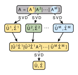
Figure 1. Flowchart for a simple (one-level) distributed parallel SVD algorithm. The different colors represent different processors completing operations in parallel.

Provided the proxy matrix is not very large, the computational and memory bottleneck of this algorithm is in the simultaneous SVD computation of the blocks $A^{i}$. If the proxy matrix is sufficiently large that the computational/memory overhead is significant, a multi-level hierarchical generalization is possible through repeated application of Lemma 1. Specifically, one could generate multiple proxy matrices by concatenating subsets of scaled left singular vectors obtained from the SVD of blocks of A, find the SVD of the proxy matrices and concatenate those singular vectors to form a new proxy matrix, and then finally recover the singular values and left singular vectors of the original matrix $A$ by finding the SVD of the proxy matrix. A visualization of this generalization is shown in Figure 2 for a two-level parallel decomposition. A general $q$-level algorithm is described in Algorithm 1.

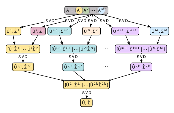
Figure 2. Flowchart for a two-level hierarchical parallel SVD algorithm. The different colors represent different processors completing operations in parallel.

Algorithm 1 A $q$-level, distributed SVD Algorithm for Highly Rectangular $A\in\mathbb{C}^{D\times N}$,   $N\gg D$.

0:  $q$ (# levels), $n$ (# local SVDs to concatenate at each level), $d\in\{1,\dots,D\}$ (intrinsic dimension), $A^{1,i}:=A^{i}\in\mathbb{C}^{D\times N_{i}}$ for $i=1,2,\ldots,M$ (block decomposition of $A$; algorithm assumes $M=n^{q}$ – generalization is trivial)

0:  $U^{\prime}\in\mathbb{C}^{D\times d}\approx$ the first $d$ columns of $U$, and $\Sigma^{\prime}\in\mathbb{R}^{d\times d}\approx\left(\Sigma\right)_{d}$.

1:  for $p=1,\dots,q$  do

2:     Compute (in parallel) the SVDs of $A^{p,i}=U^{p,i}\Sigma^{p,i}\left(V^{p,i}\right)^{*}$ for $i=1,2,\ldots,M/n^{(p-1)}$, unless the $U^{p,i}\Sigma^{p,i}$ are already available from a previous run.

3:     Set $\displaystyle A^{p+1,i}:=\left[\left(U^{p,(i-1)n+1}\Sigma^{p,(i-1)n+1}\right)_{d}~{}\Big{|}\cdots\Big{|}~{}\left(U^{p,in}\Sigma^{p,in}\right)_{d}\right]$ for $i=1,2,\ldots,M/n^{p}$.

4:  end for

5:  Compute the SVD of $A^{q+1,1}$

6:  Set $U^{\prime}:=$ the first $d$ columns of $U^{q+1,1}$, and $\Sigma^{\prime}:=\left(\Sigma^{q+1,1}\right)_{d}$.

Remark 2.

The right singular vectors can be computed (in parallel) if desired, once the left singular vectors and singular values are known. The master process broadcasts the left singular vectors and singular values to each process containing block $A^{i}$. Then columns of the right singular vectors can be constructed by computing $\frac{1}{\sigma_{j}}(A^{i})^{*}u_{j}$, were $A^{i}$ is the block of $A$ residing on process $i$, and $(\sigma_{j},u_{j})$ is the $j^{th}$ singular value and left singular vector respectively.

2.3. Theoretical Justification

In this section we will introduce some additional notation for the sake of convenience. For any matrix $A\in\mathbb{C}^{D\times N}$ with SVD $A=U\Sigma V^{*}$, we will let $\overline{A}:=U\Sigma=AV\in\mathbb{C}^{D\times N}$. It is important to note that $\overline{A}$ is not necessarily uniquely determined by $A$, for example, if $A$ is rank deficient and/or has repeated singular values. In these types of cases many pairs of unitary $U$ and $V$ may appear in a valid SVD of $A$. In what follows, one can consider $\overline{A}$ to be $AV$ for any such valid unitary matrix $V$. Similarly, one can always consider statements of the form $\overline{A}=\overline{B}$ as meaning that $A$ and $B$ are equivalent up to multiplication by a unitary matrix on the right. This inherent ambiguity does not effect the results below in a meaningful way. Given this notation Lemma 1 can be rephrased as follows:

Corollary 1.

Suppose that $A\in\mathbb{C}^{D\times N}$ has rank $d\in\{1,\ldots,D\}$, and let $A^{i}\in\mathbb{C}^{D\times N_{i}},i=1,2,\ldots,M$ be the block decomposition of $A$, i.e., $A=\left[A^{1}|A^{2}|\cdots|A^{M}\right]$. Since $A^{i}$ has rank at most $d$ for all $i=1,2,\ldots,M$, we have that

$$\overline{(A)_{d}}~{}=~{}\overline{A}~{}=~{}\overline{\left[\overline{A^{1}}~{}\big{|}~{}\overline{A^{2}}~{}\big{|}~{}\cdots~{}\big{|}~{}\overline{A^{M}}\right]}~{}=~{}\overline{\left[\overline{(A^{1})_{d}}~{}\big{|}~{}\overline{(A^{2})_{d}}~{}\big{|}~{}\cdots~{}\big{|}~{}\overline{(A^{M})_{d}}\right]}.$$

Proof.

To begin, we apply Lemma 1 with $A=\left[A^{1}|A^{2}|\cdots|A^{M}\right]$ and
$B=\left[\overline{A^{1}}~{}\big{|}~{}\overline{A^{2}}~{}\big{|}~{}\cdots~{}\big{|}~{}\overline{A^{M}}\right]$. As a result we learn that if $A$ has the SVD $A=U\Sigma V^{*}$, then $B$ also has a valid SVD of the form $B=(UW)\Sigma{V^{\prime}}^{*}$, where $W$ is a block diagonal unitary matrix with one unitary $h\times h$ block associated with each singular value that is repeated $h$-times (this allows for left singular vectors associated with repeated singular values to be rotated in the unitary matrix $U$). Note that the special structure of $W$ with respect to $\Sigma$ allows them to commute. Hence, we have that

$$B=(UW)\Sigma{V^{\prime}}^{*}~{}=~{}U\Sigma W{V^{\prime}}^{*}~{}=~{}U\Sigma(V^{\prime}W^{*})^{*}.$$

As a result we can see that $A=B(V^{\prime}W^{*}V^{*})$ which, in turn, guarantees that $\overline{A}=\overline{B}$. Hence,

(3) $$\overline{\left[A^{1}|A^{2}|\cdots|A^{M}\right]}=\overline{A}=\overline{B}=\overline{\left[\overline{A^{1}}~{}\big{|}~{}\overline{A^{2}}~{}\big{|}~{}\cdots~{}\big{|}~{}\overline{A^{M}}\right]}.$$

To finish, recall that $A$ has rank $d$. Thus, all it’s blocks, $A^{i}$ for $i=1,2,\ldots,M$, are also of rank at most $d$ (to see why, consider, e.g., the reduction of $A=\left[A^{1}|A^{2}|\cdots|A^{M}\right]$ to row echelon form). As a result, both $(i)$ $A=(A)_{d}$, and $(ii)$ $A^{i}=(A^{i})_{d}$ for all $i=1,2,\ldots,M$, are true. Substituting these equalities into (3) finishes the proof. ∎

We can now prove that Algorithm 1 is guaranteed to recover $\overline{A}$ when the rank of $A$ is known. The proof follows by inductively applying Corollary 1.

Theorem 1.

Suppose that $A\in\mathbb{C}^{D\times N}$ has rank $d\in\{1,\ldots,D\}$. Then, Algorithm 1 is guaranteed to recover an $A^{q+1,1}\in\mathbb{C}^{D\times N}$ such that $\overline{A^{q+1,1}}=\overline{A}$.

Proof.

We prove the theorem by induction on the level $p$. To establish the base case we note that

$$\overline{A}~{}=~{}\overline{\left[\overline{(A^{1,1})_{d}}~{}\big{|}~{}\overline{(A^{1,2})_{d}}~{}\big{|}~{}\cdots~{}\big{|}~{}\overline{(A^{1,M})_{d}}\right]}~{}=~{}\overline{\left[\overline{A^{1,1}}~{}\big{|}~{}\overline{A^{1,2}}~{}\big{|}~{}\cdots~{}\big{|}~{}\overline{A^{1,M}}\right]}$$

holds by Corollary 1. Now, for the purpose of induction, suppose that

$$\overline{A}~{}=~{}\overline{\left[\overline{(A^{p,1})_{d}}~{}\big{|}~{}\overline{(A^{p,2})_{d}}~{}\big{|}~{}\cdots~{}\big{|}~{}\overline{(A^{p,M/n^{(p-1)}})_{d}}\right]}~{}=~{}\overline{\left[\overline{A^{p,1}}~{}\big{|}~{}\overline{A^{p,2}}~{}\big{|}~{}\cdots~{}\big{|}~{}\overline{A^{p,M/n^{(p-1)}}}\right]}$$

holds for some some $p\in\{1,\dots,q\}$. Then, we can use the induction hypothesis and repartition the blocks of $\overline{A}$ to see that

$$\overline{A}~{} =~{}\overline{\left[\overline{(A^{p,1})_{d}}~{}\big{|}~{}\overline{(A^{p,2})_{d}}~{}\big{|}~{}\cdots~{}\big{|}~{}\overline{(A^{p,M/n^{(p-1)}})_{d}}\right]}$$

$$=~{}\overline{\left[\cdots~{}\Big{|}~{}\big{[}(\overline{A^{p,(i-1)n+1}})_{d}\dots(\overline{A^{p,in}})_{d}\big{]}~{}\Big{|}~{}\cdots\right]},~{}i=1,\dots,M/n^{p}$$

(4) $$=~{}\overline{\left[A^{p+1,1}~{}\big{|}~{}A^{p+1,2}~{}\big{|}~{}\cdots~{}\big{|}~{}A^{p+1,M/n^{p}}\right]},$$

where we have utilized the definition of $A^{p+1,i}$ from line 3 of Algorithm 1 to get (4). Applying Corollary 1 to the matrix in (4) now yields

$$\overline{A}~{}=~{}\overline{\left[\overline{A^{p+1,1}}~{}\big{|}~{}\overline{A^{p+1,2}}~{}\big{|}~{}\cdots~{}\big{|}~{}\overline{A^{p+1,M/n^{p}}}\right]}.$$

Finally, we finish by noting that each $\overline{A^{p+1,i}}$ will have rank at most $d$ since $\overline{A}$ is of rank $d$. Hence, we will also have $\overline{A}~{}=~{}\overline{\left[\overline{(A^{p+1,1})_{d}}~{}\big{|}~{}\overline{(A^{p+1,2})_{d}}~{}\big{|}~{}\cdots~{}\big{|}~{}\overline{(A^{p+1,M/n^{p}})_{d}}\right]}$, finishing the proof. ∎

Our next objective is to understand the accuracy of Algorithm 1 when it is called with a value of $d$ that is less than rank of $A$. To begin, we need to better understand how accurate blockwise low-rank approximations of a given matrix $A$ are. The following lemma provides an answer.

Lemma 2.

Suppose $A^{i}\in\mathbb{C}^{D\times N_{i}},i=1,2,\ldots,M$. Further, suppose matrix $A$ has block components $A=\left[A^{1}|A^{2}|\cdots|A^{M}\right]$, and $B$ has block components $B=\left[(A^{1})_{d}|(A^{2})_{d}|\cdots|(A^{M})_{d}\right]$. Then, $\|(B)_{d}-A\|_{\rm F}\leq\|(B)_{d}-B\|_{\rm F}+\|B-A\|_{\rm F}\leq 3\|(A)_{d}-A\|_{\rm F}$ holds for all $d\in\{1,\dots,D\}$.

Proof.

We have that

$$\|(B)_{d}-A\|_{\rm F} \leq\|(B)_{d}-B\|_{\rm F}+\|B-A\|_{\rm F}$$

$$\leq\|(A)_{d}-B\|_{\rm F}+\|B-A\|_{\rm F}$$

$$\leq\|(A)_{d}-A\|_{\rm F}+2\|B-A\|_{\rm F}.$$

Now letting $(A)^{i}_{d}\in\mathbb{C}^{D\times N_{i}},i=1,2,\ldots,M$ denote the $i^{\rm th}$ block of $(A)_{d}$, we can see that

$$\|B-A\|^{2}_{\rm F} =\sum^{M}_{i=1}\|(A^{i})_{d}-A^{i}\|^{2}_{\rm F}$$

$$\leq\sum^{M}_{i=1}\|(A)^{i}_{d}-A^{i}\|^{2}_{\rm F}$$

$$=\|(A)_{d}-A\|^{2}_{\rm F}.$$

Combining these two estimates now proves the desired result. ∎

We can now use Lemma 2 to prove a theorem that will help us to bound the error produced by Algorithm 1 for $q=1$ when $d$ is chosen to be less than the rank of $A$. It improves over Lemma 2 (in our setting) by not implicitly assuming to have access to any information regarding the right singular vectors of the blocks of $A$. It also demonstrates that the proposed method is stable with respect to additive errors by allowing (e.g., roundoff) errors, represented by $\Psi$, to corrupt the original matrix entries. Note that Theorem 2 is a strict generalization of Corollary 1. Corollary 1 is recovered from it when $\Psi$ is chosen to be the zero matrix, and $d$ is chosen to be the rank of $A$.

Theorem 2.

Suppose that $A\in\mathbb{C}^{D\times N}$ has block components $A^{i}\in\mathbb{C}^{D\times N_{i}},i=1,2,\ldots,M$, so that $A=\left[A^{1}|A^{2}|\cdots|A^{M}\right]$. Let $B=\left[\overline{(A^{1})_{d}}~{}\big{|}~{}\overline{(A^{2})_{d}}~{}\big{|}~{}\cdots~{}\big{|}~{}\overline{(A^{M})_{d}}\right]$, $\Psi\in\mathbb{C}^{D\times N}$, and $B^{\prime}=B+\Psi$. Then, there exists a unitary matrix $W$ such that

$$\left\|\overline{\left(B^{\prime}\right)_{d}}-AW\right\|_{\rm F}\leq 3\sqrt{2}\|(A)_{d}-A\|_{\rm F}+\left(1+\sqrt{2}\right)\|\Psi\|_{\rm F}$$

holds for all $d\in\{1,\dots,D\}$.

Proof.

Let $A^{\prime}=\left[\overline{A^{1}}~{}\big{|}~{}\overline{A^{2}}~{}\big{|}~{}\cdots~{}\big{|}~{}\overline{A^{M}}\right]$. Note that $\overline{A^{\prime}}=\overline{A}$ by Corollary 1. Thus, there exists a unitary matrix $W^{\prime\prime}$ such that $A^{\prime}=\overline{A}W^{\prime\prime}$. Using this fact in combination with the unitary invariance of the Frobenius norm, one can now see that

$$\left\|\left(B^{\prime}\right)_{d}-A^{\prime}\right\|_{\rm F}~{}=~{}\left\|\left(B^{\prime}\right)_{d}-\overline{A}W^{\prime\prime}\right\|_{\rm F}~{}=~{}\left\|\overline{\left(B^{\prime}\right)_{d}}-\overline{A}W^{\prime}\right\|_{\rm F}=\left\|\overline{\left(B^{\prime}\right)_{d}}-AW\right\|_{\rm F}$$

for some unitary matrixes $W^{\prime}$ and $W$. Hence, it suffices to bound $\left\|\left(B^{\prime}\right)_{d}-A^{\prime}\right\|_{\rm F}$.

Proceeding with this goal in mind we can see that

$$\left\|\left(B^{\prime}\right)_{d}-A^{\prime}\right\|_{\rm F}~{} \leq~{}\left\|\left(B^{\prime}\right)_{d}-B^{\prime}\right\|_{\rm F}+\left\|B^{\prime}-B\right\|_{\rm F}+\left\|B-A^{\prime}\right\|_{\rm F}$$

$$=~{}\sqrt{\sum^{D}_{j=d+1}\sigma^{2}_{j}(B+\Psi)}~{}+~{}\left\|\Psi\right\|_{\rm F}+\left\|B-A^{\prime}\right\|_{\rm F}$$

$$=~{}\sqrt{\sum^{\left\lceil\frac{D-d}{2}\right\rceil}_{j=1}\sigma^{2}_{d+2j-1}(B+\Psi)+\sigma^{2}_{d+2j}(B+\Psi)}~{}+~{}\left\|\Psi\right\|_{\rm F}+\left\|B-A^{\prime}\right\|_{\rm F}$$

$$\leq~{}\sqrt{\sum^{\left\lceil\frac{D-d}{2}\right\rceil}_{j=1}\left(\sigma_{d+j}(B)+\sigma_{j}(\Psi)\right)^{2}+\left(\sigma_{d+j}(B)+\sigma_{j+1}(\Psi)\right)^{2}}~{}+~{}\left\|\Psi\right\|_{\rm F}+\left\|B-A^{\prime}\right\|_{\rm F}$$

where the last inequality results from an application of Weyl’s inequality to the first term [19]. Utilizing the triangle inequality on the first term now implies that

$$\left\|\left(B^{\prime}\right)_{d}-A^{\prime}\right\|_{\rm F}~{} \leq~{}\sqrt{\sum^{D}_{j=d+1}2\sigma^{2}_{j}(B)}~{}+~{}\sqrt{\sum^{D}_{j=1}2\sigma^{2}_{j}(\Psi)}+\left\|\Psi\right\|_{\rm F}+\left\|B-A^{\prime}\right\|_{\rm F}$$

$$\leq~{}\sqrt{2}\left(\|(B)_{d}-B\|_{\rm F}+\|B-A^{\prime}\|_{\rm F}\right)+\left(1+\sqrt{2}\right)\|\Psi\|_{\rm F}.$$

Applying Lemma 2 to bound the first two terms now concludes the proof after noting that $\|(A^{\prime})_{d}-A^{\prime}\|_{\rm F}=\|(A)_{d}-A\|_{\rm F}$. ∎

This final theorem bounds the total error of the general $q$-level hierarchical Algorithm 1 with respect to the true matrix $A$ (up to multiplication by a unitary matrix on the right). The structure of its proof is similar to that of Theorem 1.

Theorem 3.

Let $A\in\mathbb{C}^{D\times N}$ and $q\geq 1$. Then, Algorithm 1 is guaranteed to recover an $A^{q+1,1}\in\mathbb{C}^{D\times N}$ such that $\overline{\left(A^{q+1,1}\right)_{d}}=AW+\Psi$, where $W$ is a unitary matrix, and $\|\Psi\|_{\rm F}\leq\left(\left(1+\sqrt{2}\right)^{q+1}-1\right)\|(A)_{d}-A\|_{\rm F}$.

Proof.

Within the confines of this proof we will always refer to the approximate matrix $A^{p+1,i}$ from line 3 of Algorithm 1 as

$$B^{p+1,i}:=\left[\overline{\left(B^{p,(i-1)n+1}\right)_{d}}~{}\Big{|}\cdots\Big{|}~{}\overline{\left(B^{p,in}\right)_{d}}\right],$$

for $p=1,\dots,q$, and $i=1,\dots,M/n^{p}$. Conversely, $A$ will always refer to the original (potentially full rank) matrix with block components $A=\left[A^{1}|A^{2}|\cdots|A^{M}\right]$, where $M=n^{q}$. Furthermore, $A^{p,i}$ will always refer to the error free block of the original matrix $A$ whose entries correspond to the entries included in $B^{p,i}$. Thus, $A=\left[A^{p,1}|A^{p,2}|\cdots|A^{p,M/n^{(p-1)}}\right]$ holds for all $p=1,\dots,q+1$, where

$$A^{p+1,i}:=\left[A^{p,(i-1)n+1}~{}\Big{|}\cdots\Big{|}~{}A^{p,in}\right]$$

for all $p=1,\dots,q$, and $i=1,\dots,M/n^{p}$. For $p=1$ we have $B^{1,i}=A^{i}=A^{1,i}$ for $i=1,\dots,M$ by definition as per Algorithm 1. Our ultimate goal is to bound the renamed $\overline{\left(B^{q+1,1}\right)_{d}}$ matrix from lines 5 and 6 of Algorithm 1 with respect to the original matrix $A$. We will do this by induction on the level $p$. More specifically, we will prove that

1. $\overline{\left(B^{p,i}\right)_{d}}=A^{p,i}W^{p,i}+\Psi^{p,i}$, where

2. $W^{p,i}$ is always a unitary matrix, and

3. $\|\Psi^{p,i}\|_{\rm F}\leq\left(\left(1+\sqrt{2}\right)^{p}-1\right)\left\|(A^{p,i})_{d}-A^{p,i}\right\|_{\rm F}$,

holds for all $p=1,\dots,q+1$, and $i=1,\dots,M/n^{(p-1)}$.

Note that conditions $1-3$ above are satisfied for $p=1$ since $B^{1,i}=A^{i}=A^{1,i}$ for all $i=1,\dots,M$ by definition. Thus, there exist unitary $W^{1,i}$ for all $i=1,\dots,M$ such that

$$\overline{\left(B^{1,i}\right)_{d}}~{}=~{}\overline{\left(A^{1,i}\right)_{d}}~{}=~{}\left(A^{1,i}\right)_{d}W^{1,i}~{}=~{}A^{1,i}W^{1,i}+\left(\left(A^{1,i}\right)_{d}-A^{1,i}\right)W^{1,i},$$

where $\Psi^{1,i}:=\left(\left(A^{1,i}\right)_{d}-A^{1,i}\right)W^{1,i}$ has

(5) $$\|\Psi^{1,i}\|_{\rm F}=\left\|\left(A^{1,i}\right)_{d}-A^{1,i}\right\|_{\rm F}\leq\sqrt{2}\left\|\left(A^{1,i}\right)_{d}-A^{1,i}\right\|_{\rm F}.$$

Now suppose that conditions $1-3$ hold for some $p\in\{1,\dots,q\}$. Then, one can see from condition 1 that

$$B^{p+1,i}~{} :=~{}\left[\overline{\left(B^{p,(i-1)n+1}\right)_{d}}~{}\Big{|}\cdots\Big{|}~{}\overline{\left(B^{p,in}\right)_{d}}\right]$$

$$=~{}\left[A^{p,(i-1)n+1}W^{p,(i-1)n+1}+\Psi^{p,(i-1)n+1}~{}\Big{|}\cdots\Big{|}~{}A^{p,in}W^{p,in}+\Psi^{p,in}\right]$$

$$=~{}\left[A^{p,(i-1)n+1}W^{p,(i-1)n+1}~{}\Big{|}\cdots\Big{|}~{}A^{p,in}W^{p,in}\right]+\left[\Psi^{p,(i-1)n+1}~{}\Big{|}\cdots\Big{|}~{}\Psi^{p,in}\right]$$

$$=~{}\left[A^{p,(i-1)n+1}~{}\Big{|}\cdots\Big{|}~{}A^{p,in}\right]\tilde{W}+\tilde{\Psi},$$

where $\tilde{\Psi}:=\left[\Psi^{p,(i-1)n+1}~{}\Big{|}\cdots\Big{|}~{}\Psi^{p,in}\right]$, and

$$\!\!\tilde{W}:=\!\!\!=\!\!\!\left(\!\!\begin{array}[]{c;{2pt/2pt}c;{2pt/2pt}c;{2pt/2pt}c}&&&\\ &&&\\ ~{}W^{p,(i-1)n+1}&{\bf 0}&{\bf 0}&{\bf 0}\\ \vspace{0.05in}\hfil\\ \hdashline[2pt/2pt]{\bf 0}&W^{p,(i-1)n+2}&{\bf 0}&{\bf 0}\\ \vspace{0.05in}\hfil\\ \hdashline[2pt/2pt]{\bf 0}&{\bf 0}&~{}\ddots{}&{\bf 0}\\ \vspace{0.05in}\hfil\\ \hdashline[2pt/2pt]{\bf 0}&{\bf 0}&{\bf 0}&W^{p,in}{}\end{array}\!\!\right)\!\!.$$

Note that $\tilde{W}$ is unitary since its diagonal blocks are all unitary by condition 2. Therefore, we have $B^{p+1,i}=A^{p+1,i}\tilde{W}+\tilde{\Psi}.$

We may now bound $\left\|\left(B^{p+1,i}\right)_{d}-A^{p+1,i}\tilde{W}\right\|_{\rm F}$ using a similar argument to that employed in the proof of Theorem 2.

$$\left\|\left(B^{p+1,i}\right)_{d}-A^{p+1,i}\tilde{W}\right\|_{\rm F}~{} \leq~{}\left\|\left(B^{p+1,i}\right)_{d}-B^{p+1,i}\right\|_{\rm F}+\left\|B^{p+1,i}-A^{p+1,i}\tilde{W}\right\|_{\rm F}$$

$$=~{}\sqrt{\sum^{D}_{j=d+1}\sigma^{2}_{j}\left(A^{p+1,i}\tilde{W}+\tilde{\Psi}\right)}~{}+~{}\|\tilde{\Psi}\|_{\rm F}$$

$$\leq~{}\sqrt{\sum^{D}_{j=d+1}2\sigma^{2}_{j}\left(A^{p+1,i}\tilde{W}\right)}~{}+~{}\sqrt{\sum^{D}_{j=1}2\sigma^{2}_{j}(\tilde{\Psi})}+\|\tilde{\Psi}\|_{\rm F}$$

(6) $$=~{}\sqrt{2}\left\|A^{p+1,i}-\left(A^{p+1,i}\right)_{d}\right\|_{\rm F}+\left(1+\sqrt{2}\right)\|\tilde{\Psi}\|_{\rm F}.$$

Appealing to condition 3 in order to bound $\|\tilde{\Psi}\|_{\rm F}$ we obtain

$$\|\tilde{\Psi}\|^{2}_{\rm F}~{}=~{}\sum^{n}_{j=1}\|\Psi^{p,(i-1)n+j}\|^{2}_{\rm F} \leq\left(\left(1+\sqrt{2}\right)^{p}-1\right)^{2}\sum^{n}_{j=1}\left\|(A^{p,(i-1)n+j})_{d}-A^{p,(i-1)n+j}\right\|^{2}_{\rm F}$$

$$\leq\left(\left(1+\sqrt{2}\right)^{p}-1\right)^{2}\sum^{n}_{j=1}\left\|(A^{p+1,i})^{j}_{d}-A^{p,(i-1)n+j}\right\|^{2}_{\rm F},$$

where $(A^{p+1,i})^{j}_{d}$ denotes the block of $(A^{p+1,i})_{d}$ corresponding to $A^{p,(i-1)n+j}$ for $j=1,\dots,n$. Thus, we have that

$$\|\tilde{\Psi}\|^{2}_{\rm F} \leq\left(\left(1+\sqrt{2}\right)^{p}-1\right)^{2}\sum^{n}_{j=1}\left\|(A^{p+1,i})^{j}_{d}-A^{p,(i-1)n+j}\right\|^{2}_{\rm F}$$

(7) $$=\left(\left(1+\sqrt{2}\right)^{p}-1\right)^{2}\left\|(A^{p+1,i})_{d}-A^{p+1,i}\right\|^{2}_{\rm F}.$$

Combining (6) and (7) we can finally see that

$$\left\|\left(B^{p+1,i}\right)_{d}-A^{p+1,i}\tilde{W}\right\|_{\rm F} \leq\left[\sqrt{2}+(1+\sqrt{2})\left(\left(1+\sqrt{2}\right)^{p}-1\right)\right]\left\|\left(A^{p+1,i}\right)_{d}-A^{p+1,i}\right\|_{\rm F}$$

(8) $$=\left(\left(1+\sqrt{2}\right)^{p+1}-1\right)\left\|\left(A^{p+1,i}\right)_{d}-A^{p+1,i}\right\|_{\rm F}.$$

Note that $\left\|\left(B^{p+1,i}\right)_{d}-A^{p+1,i}\tilde{W}\right\|_{\rm F}=\left\|\overline{\left(B^{p+1,i}\right)_{d}}-A^{p+1,i}W^{p+1,i}\right\|_{\rm F}$ where $W^{p+1,i}$ is unitary. Hence, we can see that conditions 1 - 3 hold for $p+1$ with $\Psi^{p+1,i}:=\overline{\left(B^{p+1,i}\right)_{d}}-A^{p+1,i}W^{p+1,i}$. ∎

Theorem 3 proves that Algorithm 1 will accurately compute low rank approximations of $\overline{A}$ whenever $q$ is chosen to be relatively small. Thus, Algorithm 1 provides a distributed and incremental method for rapidly and accurately computing any desired number of dominant singular values/left singular vectors of $A$. Furthermore, it is worth mentioning that the proof of Theorem 3 can be modified in order to prove that the $q$-level hierarchical Algorithm 1 is also robust/stable with respect to additive contamination of the initial input matrix $A$ by, e.g., round-off errors. This can be achieved most easily by noting that the inequality in (5) will still hold if $A^{i}=A^{1,i}$ is contaminated with arbitrary additive errors $E^{i}\in\mathbb{C}^{D\times N_{i}}$ having $\|E^{i}\|_{\rm F}\leq\frac{\sqrt{2}-1}{\sqrt{D-d}+1}\left\|\left(A^{1,i}\right)_{d}-A^{1,i}\right\|_{\rm F}$ for all $i=1,\dots,M$. We summarize this modification in the next lemma.

Lemma 3.

Let $i\in[M]$. Suppose that $B^{1,i}=A^{1,i}+E^{i}=A^{i}+E^{i}$ holds for $B^{1,i},A^{1,i},A^{i},E^{i}\in\mathbb{C}^{D\times N_{i}}$, where $\|E^{i}\|_{\rm F}\leq\frac{\sqrt{2}-1}{\sqrt{D-d}+1}\left\|\left(A^{1,i}\right)_{d}-A^{1,i}\right\|_{\rm F}$. Then, there exists a unitary matrix $W^{1,i}\in\mathbb{C}^{N_{i}\times N_{i}}$ such that

$$\left\|\overline{\left(B^{1,i}\right)_{d}}-A^{1,i}W^{1,i}\right\|_{\rm F}\leq\sqrt{2}\left\|\left(A^{1,i}\right)_{d}-A^{1,i}\right\|_{\rm F}.$$

In particular, the inequality in (5) will still hold with $\Psi^{1,i}:=\left[\left(B^{1,i}\right)_{d}-A^{1,i}\right]W^{1,i}$.

Proof.

We have that $\left(B^{1,i}\right)_{d}=A^{1,i}+\left[\left(B^{1,i}\right)_{d}-A^{1,i}\right]$ such that there exists unitary matrix $W^{1,i}$ with

$$\overline{\left(B^{1,i}\right)_{d}}~{}=~{}A^{1,i}W^{1,i}+\left[\left(B^{1,i}\right)_{d}-A^{1,i}\right]W^{1,i}.$$

As a result we have that

$$\left\|\overline{\left(B^{1,i}\right)_{d}}-A^{1,i}W^{1,i}\right\|_{\rm F} =\left\|\left(B^{1,i}\right)_{d}-A^{1,i}\right\|_{\rm F}$$

$$=\left\|\left(A^{1,i}+E^{i}\right)_{d}-A^{1,i}\right\|_{\rm F}$$

$$\leq\left\|\left(A^{1,i}+E^{i}\right)_{d}-(A^{1,i}+E^{i})\right\|_{\rm F}+\left\|E^{i}\right\|_{\rm F}$$

$$=\sqrt{\sum^{D}_{j=d+1}\sigma^{2}_{j}\left(A^{1,i}+E^{i}\right)}+\left\|E^{i}\right\|_{\rm F}$$

$$\leq\sqrt{\sum^{D}_{j=d+1}\left(\sigma_{j}\left(A^{1,i}\right)+\sigma_{1}\left(E^{i}\right)\right)^{2}}+\left\|E^{i}\right\|_{\rm F}$$

$$\leq\left\|\left(A^{1,i}\right)_{d}-A^{1,i}\right\|_{\rm F}+(1+\sqrt{D-d})\left\|E^{i}\right\|_{\rm F},$$

where the last two inequalities utilize Weyl’s inequality and the triangle inequality, respectively. The desired result now follows from our assumed bound on $\|E^{i}\|_{\rm F}$. ∎

Combining Lemma 3 with the proof of Theorem 3 allows one to see that the statement of Theorem 3 will continue to hold even when $A$ is contaminated with small additive errors. Having proven that Algorithm 1 is accurate, we are now free to consider its computational costs.

2.4. Parallel Cost Model and Collectives

To analyze the parallel communication cost of the hierarchical SVD algorithm, the $\alpha$ – $\beta$ – $\gamma$ model for distributed–memory parallel computation [9] is used. The parameters $\alpha$ and $\beta$ respectively represent the latency cost and the transmission cost of sending a floating point number between two processors. The parameter $\gamma$ represents the time for one floating point operation (FLOP).

The $q$-level hierarchical Algorithm 1 seeks to find the $d$ largest singular values and left singular vectors of a matrix $A$. If the matrix $A$ is decomposed into $M=n^{q}$ blocks, where $n$ being the number of local SVDs being concatenated at each level, the send/receive communication cost for the algorithm is

$$q\left(\alpha+d\,(n-1)\,D\beta\right),$$

assuming that the data is already distributed on the compute nodes and no scatter command is required. If the (distributed) right singular vectors are needed, then a broadcast of the left singular vectors to all nodes incurs a communication cost of $\alpha+d\,M\,\beta$.

Suppose $A$ is a $D\times N$ matrix, $N\gg D$. The sequential SVD is typically performed in two phases: bidiagonalization (which requires $(2N\,D^{2}+2D^{3})$ flops) followed by diagonalization (negligible cost). If $M$ processing cores are available to compute the $q$-level hierarchical SVD method in Algorithm 1, and the matrix $A$ is decomposed into $M=n^{q}$ blocks, where $n$ is again the number of local SVDs being concatenated at each level. The potential parallel speedup can be approximated by

(9) $$\begin{cases}\displaystyle\frac{(2ND^{2}+2D^{3})\gamma}{\gamma\left[(2(N/M)D^{2}+2D^{3})+q(2dnD^{2}+2D^{3})\right]+q(\alpha+d(n-1)D\beta)}.&\text{if }nd>D\\ \displaystyle\frac{(2ND^{2}+2D^{3})\gamma}{\gamma\left[(2(N/M)D^{2}+2D^{3})+q(2(dn)^{2}D+2(dn)^{3})\right]+q(\alpha+d(n-1)D\beta)}.&\text{if }nd<D\end{cases}$$

3. Numerical Experiments

The numerical experiments are organized into two categories. First, Theorems 1 and 3 are validated – the numerical experiments will demonstrate that the incremental algorithms can recover full rank and low rank approximations of $A$, up to rounding errors. Then, numerical evidence is presented to show the weak and strong scaling behavior of the algorithms.

3.1. Accuracy

In this first experiment, we verify that singular values and the left singular vectors of $A$ can be recovered using the incremental SVD algorithm. A full rank matrix of size $400\times 128,000$ is constructed in MATLAB, and its SVD computed to form the reference solution. The numerical experiment consists of partitioning the full matrix into various block configurations before applying the incremental SVD algorithm and comparing the singular values and left singular vectors to the reference solution. The scenarios and results are reported in Table 1: $e_{\sigma}$ refers to the maximum relative error of the singular values, i.e.,

$$\max_{1\leq i\leq D}\frac{|\tilde{\sigma}_{i}-\sigma_{i}|}{|\sigma_{i}|},$$

where $\sigma_{i}$ is the true singular value and $\tilde{\sigma}_{i}$ is the singular value obtained using the hierarchical algorithm. Similarly, $e_{v}$ refers to the maximum relative error of all the left singular vectors, i.e.,

$$\max_{1\leq i\leq D}\frac{\|\tilde{v}_{i}-v_{i}\|_{2}}{\|v_{i}\|_{2}}~{}=~{}\max_{1\leq i\leq D}\|\tilde{v}_{i}-v_{i}\|_{2},$$

where $v_{i}$ is the true singular value and $\tilde{v}_{i}$ is the singular vector obtained using the hierarchical algorithm. The number of blocks is $n^{q}$, where $q$ is the number of levels, and $n$ is the number of sketches to merge at each level. The incremental algorithm recovers the singular values and left singular vectors of a full rank matrix $A$, up to round-off errors.

$n$	levels	# blocks	block size	$e_{\sigma}$	$e_{v}$
2	1	2	$400\times 64,000$	$2.4\times 10^{-13}$	$2.3\times 10^{-12}$
	2	4	$400\times 32,000$	$1.4\times 10^{-13}$	$1.1\times 10^{-12}$
	3	8	$400\times 16,000$	$6.1\times 10^{-14}$	$2.2\times 10^{-12}$
	4	16	$400\times 8,000$	$5.3\times 10^{-14}$	$4.3\times 10^{-12}$
	5	32	$400\times 4,000$	$6.4\times 10^{-14}$	$4.3\times 10^{-12}$
	6	64	$400\times 2,000$	$5.1\times 10^{-14}$	$1.1\times 10^{-12}$
	7	128	$400\times 1,000$	$1.5\times 10^{-13}$	$1.5\times 10^{-12}$
	8	256	$400\times 500$	$1.6\times 10^{-13}$	$4.8\times 10^{-12}$
4	1	4	$400\times 16000$	$2.3\times 10^{-14}$	$3.0\times 10^{-12}$
	2	16	$400\times 1000$	$2.3\times 10^{-14}$	$2.0\times 10^{-12}$
	3	256	$400\times 125$	$1.2\times 10^{-14}$	$2.5\times 10^{-12}$

Table 1. The number of blocks is $n^{q}$, where $q$ is the number of levels, and $n$ is the number of sketches to merge at each level. The maximum relative error of the singular values $\sigma$ and left singular vectors $v$ are reported. The incremental algorithm recovers the singular values and left singular vectors of a full rank matrix $A$, up to round-off errors.

In the second experiment, the incremental SVD algorithm is used to recover a rank $d$ approximation, $(A)_{d}$, of a matrix, $A$. The matrix $A$ is again of size $400\times 128,000$, and is formed by taking the product $U\Sigma V^{\prime}$, where $U$ and $V$ are random orthogonal matrices of the appropriate size. The singular values are chosen so that $\|(A)_{d}-A\|_{F}^{2}$ can be controlled. The scenarios and results are reported in Table 2. Again, the hierarchical algorithm recovers largest $d$ singular values and associated left singular vectors to high accuracy.

$\|A-(A)_{d}\|_{F}^{2}$	$n$	levels	# blocks	block size	$e_{\sigma}$	$e_{v}$
0.1	2	1	2	$400\times 64,000$	$2.3\times 10^{-13}$	$8.3\times 10^{-9}$
		2	4	$400\times 32,000$	$1.5\times 10^{-12}$	$2.1\times 10^{-8}$
		3	8	$400\times 16,000$	$1.0\times 10^{-11}$	$5.5\times 10^{-8}$
		4	16	$400\times 8,000$	$3.7\times 10^{-11}$	$1.1\times 10^{-7}$
		5	32	$400\times 4,000$	$1.4\times 10^{-10}$	$2.0\times 10^{-7}$
		6	64	$400\times 2,000$	$3.8\times 10^{-10}$	$3.3\times 10^{-7}$
		7	128	$400\times 1,000$	$2.7\times 10^{-9}$	$7.9\times 10^{-7}$
		8	256	$400\times 500$	$9.9\times 10^{-9}$	$1.3\times 10^{-6}$
	4	1	4	$400\times 16000$	$1.5\times 10^{-12}$	$2.1\times 10^{-8}$
		2	16	$400\times 1000$	$3.7\times 10^{-11}$	$1.3\times 10^{-7}$
		3	256	$400\times 125$	$3.7\times 10^{-10}$	$3.2\times 10^{-7}$
0.01	2	1	2	$400\times 64,000$	$2.1\times 10^{-14}$	$8.2\times 10^{-12}$
		2	4	$400\times 32,000$	$8.9\times 10^{-15}$	$2.1\times 10^{-11}$
		3	8	$400\times 16,000$	$5.7\times 10^{-15}$	$5.5\times 10^{-11}$
		4	16	$400\times 8,000$	$7.4\times 10^{-15}$	$1.0\times 10^{-10}$
		5	32	$400\times 4,000$	$1.6\times 10^{-14}$	$2.5\times 10^{-10}$
		6	64	$400\times 2,000$	$3.7\times 10^{-14}$	$3.2\times 10^{-10}$
		7	128	$400\times 1,000$	$2.8\times 10^{-13}$	$7.8\times 10^{-10}$
		8	256	$400\times 500$	$9.6\times 10^{-13}$	$1.2\times 10^{-9}$
	4	1	4	$400\times 32,000$	$1.7\times 10^{-14}$	$2.1\times 10^{-11}$
		2	16	$400\times 8,000$	$1.2\times 10^{-14}$	$1.0\times 10^{-10}$
		3	256	$400\times 500$	$1.4\times 10^{-14}$	$3.1\times 10^{-10}$

Table 2. Low rank approximation of $A$ computed using the incremental SVD algorithm, compared against the true low rank approximation of $A$.

3.2. Parallel Scaling

For the first scaling experiment, the left singular vectors and the singular values of a matrix $A$ ($D=d=800$, $N=1,152,000$) are found using an MPI implementation of our hierarchical algorithm, and a threaded LAPACK SVD algorithm, dgesvd, implemented in the threaded Intel MKL library. Computational nodes from the stampede cluster at the Texas Advanced Computing Center (TACC) were used for the parallel scaling experiments. Each node is outfitted with 32GB of RAM and two Intel Xeon E5-2680 processors for a total of 16 processing cores per node. In a pre-processing step, the matrix $A$ is decomposed, with each block of $A$ stored in separate HDF5 files; the generated HDF5 files are hosted on the high-speed Lustre server. The observed speedup is summarized in Figure 3 . In the blue curve, the observed speedup is reported for a varying number of MKL worker threads. In the red curve, the speedup is reported for a varying number of worker threads $i$, applied to an appropriate decomposition of the matrix. Each worker uses the same Intel MKL library to compute the SVD of the decomposed matrices (each using a single thread), the proxy matrix is assembled, and the master thread computes the SVD of the proxy matrix using the Intel MKL library, again with a single thread. The parallel performance of our distributed SVD is superior to the threaded MKL library, this in spite of the fact that our algorithm was implemented using MPI 2.0 and does not leverage the inter-node communication savings that is possible with newer MPI implementations.

Figure 3. Strong scaling study of the dgesvd function in the threaded Intel MKL library (blue) and the proposed distributed SVD algorithm (red). The input matrix is of size $800\times 1,152,000$.

The second parallel scaling experiment is a weak scaling study, where the size of the input matrix $A$ is varied depending on the number of computing cores, $A=2000\times 32,000M$, where $M$ is the number of compute cores. The theoretical peak efficiency is computed using equation 9, assuming negligible communication overhead (i.e., we set $\alpha=\beta=0$). There is slightly better efficiency if one merges for larger $n$ (more sketches are merged together at each level). This behavior will persist until the size of the proxy matrix is comparable or larger than the original blocksize. The asymptotic behavior of the efficiency curves agree with the theoretical peak efficiency curve if $M>16$.

Figure 4. Weak scaling study of the one-level SVD algorithm. The input matrix is of size $2000\times(32000M)$, where $M$ is the processing cores used in the computation. The observed efficiency is plotted for various $n$’s (number of scaled singular vectors concatenated at each hierarchical level). There is a slight efficiency gain when increasing $n$.

In the last experiment, we repeat the weak scaling study (where the size of the input matrix $A$ is varied depending on the number of worker nodes, $A=2000\times 32,000M$, where $M$ is the number of compute cores, but utilize a priori knowledge that the rank of $A$ is much less than the ambient dimension. Specifically, we construct a data set with $d=200\ll 2000$. The hierarchical SVD performs more efficiently if the intrinsic dimension of the data can be estimated a priori. Similar observations can be made to the previous experiment: the asymptotic behavior of the efficiency curves agree with the theoretical peak efficiency curve if $M>16$.

Figure 5. Weak scaling study of the hierarchical SVD algorithm applied to data with intrinsic dimension much lower than the ambient dimension. The input matrix is of size $2000\times(32000M)$, where $M$ is the processing cores used in the computation. The intrinsic dimension is $d=200\ll 2000$. The observed efficiency is plotted for various $n$’s (number of scaled singular vectors concatenated at each hierarchical level). As expected, the theoretical and observed efficiency are better if the intrinsic dimension is known (or can be estimated) a priori.

4. Concluding Remarks and Acknowledgments

In this paper, we show that the SVD of a matrix can be constructed efficiently in a hierarchical approach. Our algorithm is proven to recover exactly the singular values and left singular vectors if the rank of the matrix $A$ is known. Further, the hierarchical algorithm can be used to recover the $d$ largest singular values and left singular vectors with bounded error. We also show that the proposed method is stable with respect to roundoff errors or corruption of the original matrix entries. Numerical experiments validate the proposed algorithms and parallel cost analysis.

The authors note that the practicality of the hierarchical algorithm is questionable for sparse input matrices, since the assembled proxy matrices as posed will be dense. Further investigation in this direction is required, but beyond the scope of this paper. Lastly, the hierarchical algorithm has a map–reduce flavor that will lend itself well to a map reduce framework such as Apache Hadoop [34] or Apache Spark [36].

Appendix A Raw data from numerical experiments

This section contains raw data used to generate the speedup curves in Section 3 for the parallel scaling studies. The simulations were conducted on the stampede cluster at the Texas Advanced Computing Center (TACC). Each node is outfitted with 32GB of RAM and two Intel Xeon E5-2680 processors for a total of 16 processing cores per node. The performance application programming interface (PAPI) [6] was used to obtain an estimate of the computational throughput obtained by the implementations.

# threads	Walltime (s)	Speedup	MFLOP/$\mu$s∗
1	245	–	40
2	151	1.6	68
3	110	2.2	100
4	91	2.6	126
8	71	3.5	194
16	71	3.5	224

Table 3. Raw data used to compute the speedup curve for Figure 3 using the threaded MKL dgesvd implementation. The reported MFLOP/$\mu$s is estimated by scaling the throughput of the master thread reported by PAPI. PAPI is unable to report the total MFLOP/$\mu$s since the MKL library uses pthreads to spawn and remove threads as needed.

$n$	levels	# blocks	block size	Walltime (s)	Speedup	MFLOP/$\mu$s
1	1	1	$800\times 1,152,000$	245	–	40
2	1	2	$800\times 768,000$	126	1.9	81
3	1	3	$800\times 512,000$	97	2.5	105
4	1	4	$800\times 384,000$	76	3.2	136
8	1	8	$800\times 192,000$	52	4.7	204
16	1	16	$800\times 96,000$	25	9.8	447

Table 4. Raw data used to compute the speedup curve for Figure 3 using the incremental SVD implementation.

$n$	levels	# blocks	Walltime (s)	Efficiency	MFLOP/$\mu$s
2	0	1	32	1	25
	1	2	41	0.78	46
	2	4	58	0.55	74
	3	8	84	0.38	110
	4	16	101	0.32	185
	5	32	121	0.26	314
	6	64	138	0.23	552
	7	128	172	0.19	907
	8	256	195	0.16	1641
	9	512	218	0.15	2928
3	0	1	32	1	25
	1	3	46	0.70	63
	2	9	74	0.43	127
	3	27	94	0.34	305
	4	81	113	0.28	767
	5	243	148	0.22	1819
4	0	1	32	1	25
	1	4	49	0.65	78
	2	16	77	0.42	209
	3	64	99	0.32	660
	4	256	131	0.24	2041

Table 5. Raw data used to compute the efficiency curves for Figure 4 using the hierarchical SVD implementation. Each block is of size $2000\times 32,000$. In this experiment, all 2000 singular values and left singular vectors are computed.

$n$	levels	# blocks	Walltime (s)	Efficiency	MFLOP/$\mu$s
2	0	1	28	1	29
	1	2	32	0.88	51
	2	4	38	0.74	90
	3	8	51	0.55	135
	4	16	52	0.54	268
	5	32	53	0.53	528
	6	64	53	0.53	1041
	7	128	54	0.52	2056
	8	256	55	0.51	4065
	9	512	58	0.48	7889
3	0	1	28	1	29
	1	3	35	0.80	72
	2	9	51	0.55	151
	3	27	52	0.54	445
	4	81	53	0.53	1322
	5	243	54	0.52	3905
4	0	1	28	1	29
	1	4	38	0.74	89
	2	16	53	0.53	264
	3	64	54	0.52	1021
	4	256	56	0.50	3940

Table 6. Raw data used to compute the efficiency curves for Figure 5 using the hierarchical SVD implementation. Each block is of size $2000\times 32,000$. In this experiment, the input matrix is of rank $d=200$; the hierarchical algorithm finds the 200 singular values and left singular vectors.

References

- [1] E. Agullo, J. Demmel, J. Dongarra, B. Hadri, J. Kurzak, J. Langou, H. Ltaief, P. Luszczek, and S. Tomov, Numerical linear algebra on emerging architectures: The plasma and magma projects, Journal of Physics: Conference Series, 180 (2009), p. 012037, http://stacks.iop.org/1742-6596/180/i=1/a=012037.
- [2] W. K. Allard, G. Chen, and M. Maggioni, Multi-scale geometric methods for data sets II: Geometric multi-resolution analysis, Appl. Comput. Harmon. Anal., 32 (2012), pp. 435–462, \hrefhttp://dx.doi.org/10.1016/j.acha.2011.08.001doi:\nolinkurl10.1016/j.acha.2011.08.001, http://dx.doi.org/10.1016/j.acha.2011.08.001.
- [3] C. G. Baker, K. A. Gallivan, and P. Van Dooren, Low-rank incremental methods for computing dominant singular subspaces, Linear Algebra Appl., 436 (2012), pp. 2866–2888, \hrefhttp://dx.doi.org/10.1016/j.laa.2011.07.018doi:\nolinkurl10.1016/j.laa.2011.07.018, http://dx.doi.org/10.1016/j.laa.2011.07.018.
- [4] L. Balzano and S. J. Wright, On grouse and incremental svd, in Computational Advances in Multi-Sensor Adaptive Processing (CAMSAP), 2013 IEEE 5th International Workshop on, Dec 2013, pp. 1–4, \hrefhttp://dx.doi.org/10.1109/CAMSAP.2013.6713992doi:\nolinkurl10.1109/CAMSAP.2013.6713992.
- [5] M. Brand, Fast low-rank modifications of the thin singular value decomposition, Linear Algebra Appl., 415 (2006), pp. 20–30, \hrefhttp://dx.doi.org/10.1016/j.laa.2005.07.021doi:\nolinkurl10.1016/j.laa.2005.07.021, http://dx.doi.org/10.1016/j.laa.2005.07.021.
- [6] S. Browne, J. Dongarra, N. Garner, G. Ho, and P. Mucci, A portable programming interface for performance evaluation on modern processors, International Journal of High Performance Computing Applications, 14 (2000), pp. 189–204, \hrefhttp://dx.doi.org/10.1177/109434200001400303doi:\nolinkurl10.1177/109434200001400303, http://hpc.sagepub.com/content/14/3/189.abstract, \hrefhttp://arxiv.org/abs/http://hpc.sagepub.com/content/14/3/189.full.pdf+htmlarXiv:http://hpc.sagepub.com/content/14/3/189.full.pdf+html.
- [7] J. R. Bunch and C. P. Nielsen, Updating the singular value decomposition, Numer. Math., 31 (1978/79), pp. 111–129, \hrefhttp://dx.doi.org/10.1007/BF01397471doi:\nolinkurl10.1007/BF01397471, http://dx.doi.org/10.1007/BF01397471.
- [8] J. R. Bunch, C. P. Nielsen, and D. C. Sorensen, Rank-one modification of the symmetric eigenproblem, Numer. Math., 31 (1978/79), pp. 31–48, \hrefhttp://dx.doi.org/10.1007/BF01396012doi:\nolinkurl10.1007/BF01396012, http://dx.doi.org/10.1007/BF01396012.
- [9] E. Chan, M. Heimlich, A. Purkayastha, and R. van de Geijn, Collective communication: theory, practice, and experience, Concurrency and Computation: Practice and Experience, 19 (2007), pp. 1749–1783, \hrefhttp://dx.doi.org/10.1002/cpe.1206doi:\nolinkurl10.1002/cpe.1206, http://dx.doi.org/10.1002/cpe.1206.
- [10] L. De Lathauwer, B. De Moor, and J. Vandewalle, A multilinear singular value decomposition, SIAM J. Matrix Anal. Appl., 21 (2000), pp. 1253–1278 (electronic), \hrefhttp://dx.doi.org/10.1137/S0895479896305696doi:\nolinkurl10.1137/S0895479896305696, http://dx.doi.org/10.1137/S0895479896305696.
- [11] R. D. Degroat, Noniterative subspace tracking, IEEE Transactions on Signal Processing, 40 (1992), pp. 571–577, \hrefhttp://dx.doi.org/10.1109/78.120800doi:\nolinkurl10.1109/78.120800.
- [12] J. Demmel, L. Grigori, M. Hoemmen, and J. Langou, Communication-optimal parallel and sequential QR and LU factorizations, SIAM J. Sci. Comput., 34 (2012), pp. A206–A239, \hrefhttp://dx.doi.org/10.1137/080731992doi:\nolinkurl10.1137/080731992, http://dx.doi.org/10.1137/080731992.
- [13] G. Golub and W. Kahan, Calculating the singular values and pseudo-inverse of a matrix, Journal of the Society for Industrial and Applied Mathematics Series B Numerical Analysis, 2 (1965), pp. 205–224, \hrefhttp://dx.doi.org/10.1137/0702016doi:\nolinkurl10.1137/0702016, http://dx.doi.org/10.1137/0702016, \hrefhttp://arxiv.org/abs/http://dx.doi.org/10.1137/0702016arXiv:http://dx.doi.org/10.1137/0702016.
- [14] G. H. Golub, Some modified matrix eigenvalue problems, SIAM Rev., 15 (1973), pp. 318–334.
- [15] M. Gu and S. C. Eisenstat, Downdating the singular value decomposition, SIAM Journal on Matrix Analysis and Applications, 16 (1995), pp. 793–810, \hrefhttp://dx.doi.org/10.1137/S0895479893251472doi:\nolinkurl10.1137/S0895479893251472, http://dx.doi.org/10.1137/S0895479893251472, \hrefhttp://arxiv.org/abs/http://dx.doi.org/10.1137/S0895479893251472arXiv:http://dx.doi.org/10.1137/S0895479893251472.
- [16] M. Gu, Stanley, S. C. Eisenstat, and I. O, A stable and fast algorithm for updating the singular value decomposition, tech. report, Yale, 1994.
- [17] A. Haidar, J. Kurzak, and P. Luszczek, An improved parallel singular value algorithm and its implementation for multicore hardware, in Proceedings of the International Conference on High Performance Computing, Networking, Storage and Analysis, SC ’13, New York, NY, USA, 2013, ACM, pp. 90:1–90:12, \hrefhttp://dx.doi.org/10.1145/2503210.2503292doi:\nolinkurl10.1145/2503210.2503292, http://doi.acm.org/10.1145/2503210.2503292.
- [18] N. Halko, P. G. Martinsson, and J. A. Tropp, Finding structure with randomness: probabilistic algorithms for constructing approximate matrix decompositions, SIAM Rev., 53 (2011), pp. 217–288, \hrefhttp://dx.doi.org/10.1137/090771806doi:\nolinkurl10.1137/090771806, http://dx.doi.org/10.1137/090771806.
- [19] R. A. Horn and C. R. Johnson, Topics in matrix analysis, Cambridge University Press, Cambridge, 1994. Corrected reprint of the 1991 original.
- [20] E. R. Jessup and D. C. Sorensen, A parallel algorithm for computing the singular value decomposition of a matrix, SIAM Journal on Matrix Analysis and Applications, 15 (1994), pp. 530–548, \hrefhttp://dx.doi.org/10.1137/S089547989120195Xdoi:\nolinkurl10.1137/S089547989120195X, http://dx.doi.org/10.1137/S089547989120195X, \hrefhttp://arxiv.org/abs/http://dx.doi.org/10.1137/S089547989120195XarXiv:http://dx.doi.org/10.1137/S089547989120195X.
- [21] I. T. Jolliffe, Principal component analysis, Springer Series in Statistics, Springer-Verlag, New York, second ed., 2002.
- [22] T. G. Kolda, G. Ballard, and W. N. Austin, Parallel Tensor Compression for Large-Scale Scientific Data., Sandia National Laboratories, Oct 2015, \hrefhttp://dx.doi.org/10.2172/1226255doi:\nolinkurl10.2172/1226255, http://www.osti.gov/scitech/servlets/purl/1226255.
- [23] J. T. Kwok and H. Zhao, Incremental eigen decomposition, in IN PROC. ICANN, 2003, pp. 270–273.
- [24] Y. Li, On incremental and robust subspace learning, Pattern Recognition, 37 (2004), pp. 1509 – 1518, \hrefhttp://dx.doi.org/http://dx.doi.org/10.1016/j.patcog.2003.11.010doi:\nolinkurlhttp://dx.doi.org/10.1016/j.patcog.2003.11.010, http://www.sciencedirect.com/science/article/pii/S003132030300431X.
- [25] F. Liu and F. Seinstra, Adaptive parallel householder bidiagonalization, in Euro-Par 2009 Parallel Processing, H. Sips, D. Epema, and H.-X. Lin, eds., vol. 5704 of Lecture Notes in Computer Science, Springer Berlin Heidelberg, 2009, pp. 821–833, \hrefhttp://dx.doi.org/10.1007/978-3-642-03869-3_76doi:\nolinkurl10.1007/978-3-642-03869-3_76, http://dx.doi.org/10.1007/978-3-642-03869-3_76.
- [26] F. Liu and F. J. Seinstra, Gpu-based parallel householder bidiagonalization, in Proceedings of the 19th ACM International Symposium on High Performance Distributed Computing, HPDC ’10, New York, NY, USA, 2010, ACM, pp. 288–291, \hrefhttp://dx.doi.org/10.1145/1851476.1851512doi:\nolinkurl10.1145/1851476.1851512, http://doi.acm.org/10.1145/1851476.1851512.
- [27] H. Ltaief, P. Luszczek, and J. Dongarra, High-performance bidiagonal reduction using tile algorithms on homogeneous multicore architectures, ACM Trans. Math. Softw., 39 (2013), pp. 16:1–16:22, \hrefhttp://dx.doi.org/10.1145/2450153.2450154doi:\nolinkurl10.1145/2450153.2450154, http://doi.acm.org/10.1145/2450153.2450154.
- [28] P. Ma, M. W. Mahoney, and B. Yu, A statistical perspective on algorithmic leveraging, J. Mach. Learn. Res., 16 (2015), pp. 861–911.
- [29] X. Meng, J. K. Bradley, B. Yavuz, E. R. Sparks, S. Venkataraman, D. Liu, J. Freeman, D. B. Tsai, M. Amde, S. Owen, D. Xin, R. Xin, M. J. Franklin, R. Zadeh, M. Zaharia, and A. Talwalkar, MLlib: Machine Learning in Apache Spark, CoRR, abs/1505.06807 (2015), http://arxiv.org/abs/1505.06807.
- [30] M. Moonen, P. V. Dooren, and J. Vandewalle, A singular value decomposition updating algorithm for subspace tracking, SIAM Journal on Matrix Analysis and Applications, 13 (1992), pp. 1015–1038, \hrefhttp://dx.doi.org/10.1137/0613061doi:\nolinkurl10.1137/0613061, http://dx.doi.org/10.1137/0613061, \hrefhttp://arxiv.org/abs/http://dx.doi.org/10.1137/0613061arXiv:http://dx.doi.org/10.1137/0613061.
- [31] I. V. Oseledets, Tensor-train decomposition, SIAM J. Sci. Comput., 33 (2011), pp. 2295–2317, \hrefhttp://dx.doi.org/10.1137/090752286doi:\nolinkurl10.1137/090752286, http://dx.doi.org/10.1137/090752286.
- [32] D. Skoc̆aj and A. Leonardis, Incremental and robust learning of subspace representations, Image and Vision Computing, 26 (2008), pp. 27 – 38, \hrefhttp://dx.doi.org/http://dx.doi.org/10.1016/j.imavis.2005.07.028doi:\nolinkurlhttp://dx.doi.org/10.1016/j.imavis.2005.07.028, http://www.sciencedirect.com/science/article/pii/S0262885606000679. Cognitive Vision-Special Issue.
- [33] G. W. Stewart, An updating algorithm for subspace tracking, IEEE Transactions on Signal Processing, 40 (1992), pp. 1535–1541, \hrefhttp://dx.doi.org/10.1109/78.139256doi:\nolinkurl10.1109/78.139256.
- [34] T. White, Hadoop: The Definitive Guide, O’Reilly Media, Inc., 1st ed., 2009.
- [35] M. Zaharia, M. Chowdhury, T. Das, A. Dave, J. Ma, M. McCauley, M. J. Franklin, S. Shenker, and I. Stoica, Resilient distributed datasets: A fault-tolerant abstraction for in-memory cluster computing, in Proceedings of the 9th USENIX Conference on Networked Systems Design and Implementation, NSDI’12, Berkeley, CA, USA, 2012, USENIX Association, pp. 2–2, http://dl.acm.org/citation.cfm?id=2228298.2228301.
- [36] M. Zaharia, M. Chowdhury, M. J. Franklin, S. Shenker, and I. Stoica, Spark: Cluster computing with working sets, in Proceedings of the 2Nd USENIX Conference on Hot Topics in Cloud Computing, HotCloud’10, Berkeley, CA, USA, 2010, USENIX Association, pp. 10–10, http://dl.acm.org/citation.cfm?id=1863103.1863113.
- [37] H. Zha and H. D. Simon, On updating problems in latent semantic indexing, SIAM J. Sci. Comput., 21 (1999), pp. 782–791 (electronic), \hrefhttp://dx.doi.org/10.1137/S1064827597329266doi:\nolinkurl10.1137/S1064827597329266, http://dx.doi.org/10.1137/S1064827597329266.
- [38] H. Zhao, P. C. Yuen, and J. T. Kwok, A novel incremental principal component analysis and its application for face recognition, IEEE Transactions on Systems, Man, and Cybernetics, Part B (Cybernetics), 36 (2006), pp. 873–886, \hrefhttp://dx.doi.org/10.1109/TSMCB.2006.870645doi:\nolinkurl10.1109/TSMCB.2006.870645.