Growth of a dry spot under a vapor bubble at high heat flux and high pressure

Abstract

We report a 2D modeling of the thermal diffusion-controlled growth of a vapor bubble attached to a heating surface during saturated boiling. The heat conduction problem is solved in a liquid that surrounds a bubble with a free boundary and in a semi-infinite solid heater by the Boundary Element Method. At high system pressure the bubble is assumed to grow slowly, its shape being defined by the surface tension and the vapor recoil force, a force coming from the liquid evaporating into the bubble. It is shown that at some typical time the dry spot under the bubble begins to grow rapidly under the action of the vapor recoil. Such a bubble can eventually spread into a vapor film that can separate the liquid from the heater thus triggering the boiling crisis (Critical Heat Flux).

and

NOMENCLATURE
$\vec{a}$	arbitrary vector	$x$	abscissa
$b$	exponent for boundary meshing	$y$	ordinate
$C$	arbitrary constant	Greek letters
$c_{p}$	specific heat [J/(kg K)]	$\alpha$	thermal diffusivity [m2/s]
$d_{min}$	smallest element length [m]	$\beta$	exponent
$\vec{e}_{x},\vec{e}_{y}$	unit vectors directed along the axes	$\Delta t$	time step [s]
$F,f$	non-dimensional time	$\zeta$	reduced heat flux
Fo	Fourier number	$\eta$	rate of evaporation [kg/(s$\cdot$m2)]
$G$	Green function, BEM coefficient	$\theta$	liquid contact angle
$H$	latent heat [J/kg], BEM coefficient	$\lambda$	vapor/liquid pressure difference [N/m2]
Hi	Hickman number	$\xi$	non-dimensional curvilinear coordinate
Ja	Jakob number	$\rho$	mass density [kg/m3]
$j$	volume heat supply [W/m3]	$\sigma$	surface tension [N/m]
$K$	curvature [m-1]	$\tau$	dummy
$k$	thermal conductivity [W/(m K)]	$\psi$	reduced temperature
$L$	half-length of the bubble contour [m]	$\Omega$	2D-domain
$M$	molar weight of water [kg/mol]	$\partial\Omega$	contour of the 2D-domain
$N$	total boundary elements number	Subscripts
$\vec{n}$	internal unit normal vector	$d$	dry spot
$P_{r}$	vapor recoil pressure [N/m2]	$e$	external to the bubble
$q$	heat flux [W/m2]	$F,f$	value at time $F$ or $f$
$q_{CHF}$	critical heat flux [MW/m2]	$i$	vapor-liquid interface
$q_{0}$	control value of heat flux [MW/m2]	$i,j$	value at the node $i$ or $j$
$R$	bubble radius [m]	$inf$	at $x\rightarrow\infty$ (also as a superscript)
$R_{0}$	initial bubble radius [m]	$L$	liquid
$R_{g}$	molar gas constant [J/(mol K)]	$max$	maximum
$\vec{r}$	radius-vector	$S$	solid (heater)
$T$	temperature [K]	$sat$	saturation
$t$	time [s]	$V$	vapor
$t_{c}$	transition time [s]	$w$	wetted part of the heater
$t_{dep}$	bubble residence time [s]	Superscripts
$u$	auxiliary angle	$x$	x-component of the vector
$V$	2D-bubble volume [m2]	$y$	y-component of the vector
$v^{n}$	interface velocity [m/s]	$\;\bar{}$	reference value

1 Introduction

In nucleate boiling, a very large rate of heat transfer from the heating surface to the bulk is due to both the phase change (latent heat of vaporization) and the fact that the superheated liquid is carried away from the heating surface by the departing vapor bubbles. Therefore, the knowledge of the nucleation and growth of the bubbles on the heating surface is very important for the calculations of the heat transfer rate. Many works were focused on the bubble growth kinetics, see e.g. [1, 2, 3, 4, 5, 6]. However, as it was recently recognized [7], the behavior of the fluid in contact with the solid heater remains poorly studied. We think that this situation is due to the success of the microlayer model [2] that proved to be self-sufficient for the description of the bubble growth kinetics and the heat transfer rate. The microlayer model postulates the existence of a thin liquid film between the heater and the foot of the vapor bubble. This model is based on observations of the bubbles at low system pressures with respect to the critical pressure for the given fluid. At low pressures, the fast bubble growth creates a hydrodynamic resistance that makes the bubble almost hemispherical [8]. As proved by direct observations [9, 10] through the transparent heating surface, the dry spot (i.e. the spot of the direct contact between the liquid and the vapor) does exist around the nucleation site while the bubble stays near the heating surface. The origin of the dry spot can be explained as follows. First, it is necessary that the vapor-solid adhesion exists to avert the immediate removal of the bubble from the heater by the lift-off forces. This adhesion only appears when the vapor contacts the solid directly. Second, the strong generation of vapor at the triple contact line around the nucleation site prevents covering of the nucleation site by the liquid. As a consequence, the existence of the dry spot under the bubble is necessary during most of the time of the bubble growth, until the bubble departure from the heater.

Because of the hemispheric bubble shape, the apparent bubble foot is much larger than the dry spot. That is why the microlayer model works so well at low pressures. For high system pressure, comparable to the critical pressure (see [11, 12] for the discussion of the threshold between these two regimes), the picture is different. The bubble growth is much slower so that the hydrodynamic forces are small with respect to the surface tension. Consequently, the bubble resembles a sphere much more than a hemisphere [8]. It is very hard to identify the microlayer as a thin film in this case. In this article we will limit ourselves to this particular case.

One of the most important phenomena in boiling at the large heat fluxes used in industrial heat exchangers is the boiling crisis called alternately “burnout”, “Departure from Nucleate Boiling”, or “Critical Heat Flux” (CHF) [1, 8]. When the heat flux from the heater exceeds a critical value (the CHF), the vapor bubbles abruptly form a film that thermally insulates the heater surface from the liquid. Consequently, the temperature of the heater rapidly grows. The dry spot is recognized as playing a key role in the boiling crisis [13]. A new physical approach [14] was recently suggested by some of us to describe this phenomenon. It is based on the experimental results [9, 10] that show that the boiling crisis can begin with the fast growth of a dry spot under a single bubble, although several simultaneously spreading bubbles can coalesce later on. The model associates the onset of the boiling crisis with the beginning of the spreading of the dry spot below a vapor bubble attached to the heater surface. The purpose of the present article is to rigorously calculate in 2D the temporal evolution of the dry spot under a single bubble.

Two main difficulties arise while solving this problem. The first of them is the necessity to solve the full free-boundary problem for the bubble. Unfortunately, we cannot assume a simple shape for the bubble foot as has been done in all previous simulations of the vapor bubble growth that we are aware of, see e.g. [3, 4, 6]. The reason is that these models do not rigorously determine the size of the dry spot. Instead, they use an empirical correlation for the microlayer parameters chosen to satisfy the experimentally observed growth rate of the bubble. In the present formulation, the dry spot size is determined in a self-consistent manner from the position of the triple contact line. Such a free-boundary problem is difficult because of its non-linearity and can be solved by only a few numerical methods, e.g. Boundary Element Method (BEM) [15] or Front Tracking Method. The latter was recently used [16] to simulate the film boiling in 2D.

The second difficulty of the dry spot problem is associated with the calculation of the heat transfer in the most important region — the vicinity of the triple contact line (i.e. the microlayer). It is analyzed analytically in the subsection 3.1 for two fixed values of the contact angle. Although these results are not used in the numerical simulation, we need them to check the accuracy of the heat transfer calculation in this important region.

Our calculations are valid in the simplified situation where the hydrodynamic effects in liquid are neglected. This simplification is justified by the slow growth assumption valid for high system pressures. This approximation is common [5] for the thermal diffusion-controlled bubble growth. The only dynamic condition that cannot be neglected [14] is the dynamic balance of mechanical momentum at the bubble interface that results in the vapor recoil pressure. This approach allows us to apply the quasi-static approximation for the bubble shape determination in sec. 2 and neglect the convection terms in the heat transfer problem that is discussed in sec. 3. The numerical algorithm is described in section 4. The results of the simulation and the conclusions are presented in sections 5 and 6.

2 Bubble shape determination

When the heat flux $q_{S}$ from the heater is small, the vapor bubble grows with its triple vapor-liquid-solid contact line pinned by the surface defect on which the vapor nucleation has started. The size of the dry spot is thus very small with respect to the bubble size. According to the model [14] that should be valid for any system pressure, at some value of $q_{S}$ the contact line depins and spreads under the influence of the vapor recoil pressure $P_{r}$,

$$P_{r}=\eta^{2}(\rho_{V}^{-1}-\rho_{L}^{-1}),$$ (1)

where $\eta$ is the mass of the evaporated liquid per unit time per unit area of the vapor-liquid interface. $P_{r}$ may vary along the interface and is directed normally to this interface towards the liquid [18]. By neglecting heat conduction in the vapor with respect to the latent heat effect, $\eta$ can be related to the local heat flux across the interface $q_{L}$ by the equation

$$q_{L}=H\eta,$$ (2)

where $H$ is the latent heat of vaporization. Because of the strong temperature gradient in the vicinity of the heating surface, $q_{L}$ increases sharply near the contact line, and consequently $\eta$ and $P_{r}$ also increase. In other words, the pressure increases near the contact line and causes it to recede. Therefore, the dry spot under the bubble should grow with time.

The bubble shape is determined using a quasi-static approximation. We neglect all but two forces that define the bubble shape: the surface tension and the vapor recoil pressure $P_{r}$ defined by Eq. 1. The bubble shape is then defined by the pressure balance (see [14])

$$K\sigma=\lambda+P_{r},$$ (3)

where $K$ is the local curvature of the bubble, $\sigma$ is the vapor-liquid interface tension and $\lambda$ is a constant difference of pressures between the vapor and the liquid. $\lambda$ should be determined using the known volume $V$ of the 2D bubble. At any time, the volume $V$ of the 2D bubble (see Appendix A) can be written as:

$$V={1\over 2}\int\limits_{(\partial\Omega_{i})}(xn_{e}^{x}+yn_{e}^{y})\;{\rm d}\,\partial\Omega,$$ (4)

where $\partial\Omega_{i}$ is the vapor-liquid interface, and the external unit normal vector $\vec{n}_{e}=(n_{e}^{x},n_{e}^{y})$ to the bubble is defined in a Cartesian $(x,y)$ coordinate system. An axisymmetric bubble shape is assumed in the following, see Fig. 1.

It is convenient to describe the bubble shape in parametric form while choosing a non-dimensional length $\xi$ measured along the bubble contour as an independent variable. Then the coordinates $(x,y)$ for a given point on the bubble interface are functions of $\xi$ that varies along the bubble half-contour (its right half in Fig. 1) from 0 to 1, $\xi=0$ and $\xi=1$ corresponding to the topmost point of the bubble and to the contact point respectively. Eq. 3 for the 2D case is equivalent to the following parametric system of ordinary differential equations:

$${\rm d}x/{\rm d}\xi = L\cos u,$$ (5)

$${\rm d}y/{\rm d}\xi = -L\sin u,$$ (6)

$${\rm d}u/{\rm d}\xi = L(\lambda+P_{r}(\xi))/\sigma$$ (7)

were $u=u(\xi)$ is the angle between the tangent to $\partial\Omega_{i}$ at the point $\xi$ and the vector directed opposite to the $x$-axis; $L$ is the half-length of $\partial\Omega_{i}$.

The boundary conditions for Eqs. 5 – 7 are then given by

$$x(0)=0,\quad u(0)=0,\quad y(1)=0.$$ (8)

A 4th condition $u(1)=\pi-\theta$ that fixes the liquid contact angle $\theta$ is necessary to determine the unknown $L$ using (7):

$$L=(\pi-\theta)\sigma\left[\int\limits_{0}^{1}P_{r}(\xi){\rm d}\xi+\lambda\right]^{-1}.$$ (9)

In the following, we consider the usual case of complete wetting of the heating surface by the liquid, $\theta=0$. The solution of the problem (1 – 9) allows the bubble shape to be determined providing the heat flux through the vapor-liquid interface is known.

3 Heat transfer problem

The calculation of the heat transfer around a growing vapor bubble is a free boundary problem. To our knowledge, only two other groups have solved the full free-boundary boiling problem [16, 17]. In both works the singular effects, which appear in the region adjacent to the triple contact line (microlayer), are not discussed. However, we know that almost all the heat flux supplied to the vapor bubble goes through this particular region, a region on which we concentrate in this work. As a first step, we neglect the heat transfer due to the liquid motion. Thermal conduction and the latent heat effects are taken into account to describe the time evolution of the 2D vapor bubble. The vapor is assumed to be non-conducting. The case of saturated boiling is considered. This means that the temperature in the liquid far from the heater is equal to $T_{sat}$, the saturation temperature for the given system pressure. Thus only evaporation is allowed on the bubble interface. Since we consider a slow process with no liquid motion, the pressures are assumed to be uniform both in the vapor and in the liquid. However, they are different according to (3) where $\lambda$ is the difference between the pressures inside and outside the vapor bubble. The saturation temperature $T^{\prime}_{sat}$ for the vapor inside the bubble depends on the vapor pressure according to the Clausius-Clapeyron equation (see, e.g. [4])

$$T^{\prime}_{sat}=T_{sat}[1+{\lambda\over H}(\rho_{V}^{-1}-\rho_{L}^{-1})].$$

Since $\sigma/\lambda$ is the bubble radius at the top of the bubble (where $P_{r}$ is negligible), it is easy to estimate that the correction to $T_{sat}$ is less than $10^{-3}$% even for the smallest bubble size considered. Therefore, in the following, the bubble surface is supposed to be at constant temperature $T_{sat}$.

3.1 Model for the vicinity of the contact line

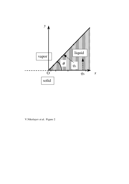
Figure 2: Geometry for the analytical calculation of the heat conduction in the wedge. The BEM discretization of the wedge is also illustrated.

First of all, we need to understand how $q_{L}$ behaves in the vicinity of the contact line where the contour of the bubble $\partial\Omega_{i}$ can be approximated by a straight line that forms an angle $\theta$ with the $Ox$ heater line, see Fig. 2. Then $q_{L}$ can be obtained from the solution of a simple two-dimensional problem of unsteady heat conduction in this wedge of liquid, the point $O(x=0,y=0)$ corresponding to the contact line. In our previous article [14] the model problem was solved to show that when $\theta=\pi/2$ and a constant heat flux from the heater is imposed, the heat flux through the liquid-vapor interface $q_{L}$ diverges weakly (logarithmically) near the contact line. In the present work we treat two cases $\theta=\pi/4$ and $\theta=\pi/8$ which also allow an analytical treatment.

The heat conduction equation for the temperature $T_{L}(x,y,t)$ in the liquid

$${\partial T_{L}\over\partial t}=\alpha_{L}\nabla^{2}T_{L}$$ (10)

has the initial and boundary conditions

$$\left.T_{L}\right|_{t=0}=T_{sat},$$ (11)

$$\left.T_{L}\right|_{\partial\Omega_{i}}=T_{sat},$$ (12)

$$-k_{L}\left.{\partial T_{L}\over\partial y}\right|_{y=0}=q_{0},$$ (13)

where $k_{L}$ and $\alpha_{L}$ are the thermal conductivity and the thermal diffusivity of the liquid, and the heat flux $q_{S}$ from the heating surface is assumed to be constant ($=q_{0}$) for the case of the thin heating wall. The solution of this 2D problem for the angles $\theta=\pi/2^{m}$, where $m$ is integer, can be obtained using the method of images [19] for the Green function. For $\theta=\pi/4$ it reads

$$T_{L}=T_{sat}+T_{inf}(y,t)-T_{inf}(x,t),$$ (14)

where the function $T_{inf}(y,t)$ is a solution for this problem at $x\rightarrow\infty$

$$T_{inf}(y,t)={q_{0}\over k_{L}}\left[\sqrt{4\alpha_{L}t\over\pi}\exp\left(-{y^{2}\over 4\alpha_{L}t}\right)-y\,\mbox{erfc}\left({y\over 2\sqrt{\alpha_{L}t}}\right)\right],$$ (15)

erfc$(z)$ being the complementary error function [20]. Then the heat flux $q_{L}$

$$q_{L}=-k_{L}(\vec{n}\cdot\nabla)\left.T_{L}\right|_{\partial\Omega_{i}}$$ (16)

can be calculated as a function of $x$ using the expression for the unit normal vector $\vec{n}=(-\sin\theta,\,\cos\theta)$:

$$q_{L}=q_{0}\sqrt{2}\,\mbox{erfc}\left({x\over 2\sqrt{\alpha_{L}t}}\right).$$ (17)

It is easy to see that, unlike the problem [14] for $\theta=\pi/2$, the heat flux remains finite at the contact line ($x=0$). This is also true for the case $\theta=\pi/8$, for which

$$T_{L}=T_{sat}+T_{inf}(y,t)+T_{inf}(x,t)-T_{inf}\left({x+y\over\sqrt{2}},t\right)-T_{inf}\left({x-y\over\sqrt{2}},t\right),$$ (18)

and

$$q_{L}=q_{0}\sqrt{\sqrt{2}+2}\left[\mbox{erfc}\left({(\sqrt{2}-1)x\over 2\sqrt{\alpha_{L}t}}\right)-(\sqrt{2}-1)\,\mbox{erfc}\left({x\over 2\sqrt{\alpha_{L}t}}\right)\right].$$ (19)

Although these solutions present important benchmarks for the numerical calculations of the heat transfer near the contact line, they cannot be used in the simulation itself for two reasons. The first is the impossibility to employ the uniform heat flux boundary condition (13) because in reality the heat flux vary strongly between the dry and wetted parts of the solid surface. In particular, the heat flux through the dry spot under a bubble is very small (we assume it to be zero in the following). The second reason is the impossibility to approximate the bubble contour by a straight line for the case $\theta=0$, most important for the industrial applications.

3.2 Mathematical formulation

We consider the growth of a vapor bubble on the semi-infinite ($y<0$) solid heater $\Omega_{S}$ in the semi-infinite ($y>0$) liquid $\Omega_{L}$, see Fig. 1. We assume that no superheat is needed for the bubble nucleation so that the circular bubble of the radius $R_{0}$ and the volume $V_{0}$ has already nucleated at the heater surface at $t=0$. The validity of this assumption is discussed in sec. 5. The known heat supply $j(t)$ is generated homogeneously inside the heater with the heat conductivity $k_{S}$ and the heat diffusivity $\alpha_{S}$ so that heat conduction equation for the domain $\Omega_{S}$

$${\partial T_{S}\over\partial t}=\alpha_{S}\nabla^{2}T_{S}+{\alpha_{S}\over k_{S}}j(t),\quad y<0$$ (20)

should be solved with the boundary and the initial conditions

$$q_{S}=-k_{S}\left.{\partial T_{S}\over\partial y}\right|_{y=0}=\left\{\begin{array}[]{lll}\displaystyle-k_{L}\left.{\partial T_{L}\over\partial y}\right.&\mbox{at}&\partial\Omega_{w}\\ 0&\mbox{at}&\partial\Omega_{d}\end{array}\right.,$$ (23)

$$\left.T_{S}\right|_{\partial\Omega_{w}}=\left.T_{L}\right|_{y=0},$$ (24)

$$\left.T_{S}\right|_{t=0}=T_{sat},$$ (25)

where $\partial\Omega_{d}$ is the vapor-solid interface (i.e. the dry spot) and $\partial\Omega_{w}$ is the liquid-solid interface(wetted surface), see Fig. 1. The problem for the domain $\Omega_{L}$ is completed by Eqs. 10 – 12.

The bubble volume $V$ increases due to evaporation [1]:

$$H\rho_{V}{{\rm d}V\over{\rm d}t}=\int\limits_{(\partial\Omega_{i})}q_{L}\;{\rm d}\,\partial\Omega,$$ (26)

where $q_{L}$ is calculated using (16) in which $\vec{n}$ is the inner normal vector to $\partial\Omega_{i}$, $\vec{n}=-\vec{n}^{e}$.

The formulated mathematical problem can be solved by the Boundary Element Method (BEM) generalized for moving boundary problems [21]. Before its direct application, we consider the integration contours for the domains $\Omega_{L}$ and $\Omega_{S}$. Obviously, they should contain $\partial\Omega_{i}$, $\partial\Omega_{d}$ and $\partial\Omega_{w}$ and a circle that closes the contours at infinity. The non-zero values of the temperature and flux at infinity complicates the solution. Therefore, we calculate these values $T_{S}^{inf}$ and $T_{L}^{inf}$ at $x\rightarrow\infty$ and then subtract them from $T_{S}$ and $T_{L}$. The resulting modified variables are zero at infinity. This transformation allows the integration contour to be reduced to $\partial\Omega_{i}\cup\partial\Omega_{d}\cup\partial\Omega_{w}$.

3.3 Solution at infinity

The solution at infinity satisfies the same problem as $T_{S}$ and $T_{L}$ but with the eliminated dependence on $x$ and $\partial\Omega_{d}=\emptyset$. The separate solutions for $y\geq 0$ and $y\leq 0$ can be easily found using the known Green function for the semi-infinite space [19]:

$$T_{L}^{inf}=T_{sat}+{\sqrt{\alpha_{L}}\over k_{L}\sqrt{\pi}}\int\limits_{0}^{t}{q_{0}(t-\tau)\over\sqrt{\tau}}\exp\left(-{y^{2}\over 4\alpha_{L}t}\right)\,{\rm d}\tau,\quad y\geq 0$$ (27)

$$T_{S}^{inf}=T_{sat}+{\alpha_{S}\over k_{S}}\int\limits_{0}^{t}j(\tau)\,{\rm d}\tau-{\sqrt{\alpha_{S}}\over k_{S}\sqrt{\pi}}\int\limits_{0}^{t}{q_{0}(t-\tau)\over\sqrt{\tau}}\exp\left(-{y^{2}\over 4\alpha_{S}t}\right)\,{\rm d}\tau,\quad y\leq 0$$ (28)

The unknown heat flux from the heater, $q_{0}(t)$, can be found for arbitrary $j(t)$ out of the integral equation that results from equality of (27) and (28) at $y=0$. It is worth mentioning that if $j\propto t^{-1/2}$, a constant $q_{0}$ satisfies this integral equation. This means that in the bubble growth problem with this choice of $j(t)$ the heat flux from the heater would remain constant at least far from the growing bubble. This choice will allow us to avoid the influence of the varying heat flux on the bubble growth and thus will be used in the following. The solution in analytical form is:

$$j(t)=C/\sqrt{t},$$

$$q_{0}=C\sqrt{\pi}\alpha_{S}k_{L}/(k_{S}\sqrt{\alpha_{L}}+k_{L}\sqrt{\alpha_{S}}),$$

$$T_{S}^{inf}=T_{sat}+{2\alpha_{S}\over k_{S}}C\sqrt{t}-{q_{0}\over k_{S}}\left[\sqrt{4\alpha_{S}t\over\pi}\exp\left(-{y^{2}\over 4\alpha_{S}t}\right)+y\,\mbox{erfc}\left(-{y\over 2\sqrt{\alpha_{S}t}}\right)\right],\quad y\leq 0,$$ (29)

$$T_{L}^{inf}=T_{sat}+T_{inf}(y,t),\quad y\geq 0,$$ (30)

where $C$ and $q_{0}$ are constant and the function $T_{inf}(y,t)$ is defined in (15). It is easy to see that besides the advantage of the zero values at infinity for the modified variables $T_{L,S}-T_{L,S}^{inf}$, the equation for both of them has the form (10) with no source term.

3.4 Non-dimensional formulation

By introducing the characteristic scales for time ($\Delta t$, the time step), length ($R_{0}$, the initial bubble radius), heat flux ($\bar{q}$), and thermal conductivity ($\bar{k}$), all other variables can be made non-dimensional. In particular, the characteristic temperature scale in the system is $\bar{q}R_{0}/\bar{k}$. The following four non-dimensional groups define completely the behavior of the system

$${\rm Fo}_{L,S}=\alpha_{L,S}\Delta t/R_{0}^{2}\mbox{ --- Fourier numbers},$$

$${\rm Ja}={\rho_{L}c_{p\,L}\over\rho_{V}H}{\bar{q}R_{0}\over\bar{k}}\mbox{ --- Jakob number\cite[cite]{[\@@bibref{}{Tong}{}{}]}},$$

$${\rm Hi}={R_{0}\,\bar{q}^{2}\over\sigma H^{2}}(\rho_{V}^{-1}-\rho_{L}^{-1})\mbox{ --- Hickman number},$$

providing that non-dimensionalized values of $q_{0}$ and $k_{L,S}$ are fixed. The following is the complete non-dimensional heat transfer problem formulated in terms of $\psi_{L,S}=(T_{L,S}-T_{L,S}^{inf})/(\bar{q}R_{0}/\bar{k})$:

$${\partial\psi_{L,S}\over\partial t}={\rm Fo}_{L,S}\nabla^{2}\psi_{L,S}$$ (31)

$$\left.\psi_{L,S}\right|_{t=0}=0,$$ (32)

$$\left.\psi_{L}\right|_{\partial\Omega_{i}}=-T_{inf}(y,t),$$ (33)

$$\left.\zeta_{L}\right|_{\partial\Omega_{w}}=\left.\zeta_{S}\right|_{\partial\Omega_{w}},\quad\zeta_{L,S}=k_{L,S}{\partial\psi_{L,S}\over\partial\vec{n}},$$ (34)

$$\left.\zeta_{L}\right|_{\partial\Omega_{d}}=-q_{0}$$ (35)

$${{\rm d}V\over{\rm d}t}={\rm Fo}_{L}\cdot{\rm Ja}\int\limits_{(\partial\Omega_{i})}(\zeta_{inf}-\zeta_{L})\;{\rm d}\,\partial\Omega,\quad\zeta_{inf}=q_{0}n^{y}\,\mbox{erfc}\left({y\over 2\sqrt{{\rm Fo}_{L}t}}\right)\quad$$ (36)

where $n^{y}$ is the ordinate of the vector $\vec{n}$ and all quantities are non-dimensionalized. The whole problem is completed using the non-dimensionalized set of equations for the bubble shape (5 – 9) where the non-dimensional expression for the vapor recoil pressure is used:

$$P_{r}={\rm Hi}(\zeta_{inf}-\zeta_{L})^{2}.$$ (37)

3.5 Boundary Element techniques applied to bubble growth

As it is shown in [21], the heat conduction problem (31 – 32) is equivalent to the set of two integral equations, written for each of the domains $\Omega_{L}$ and $\Omega_{S}$:

$$\int\limits_{0}^{t_{F}}{\rm d}t\int\limits_{(\partial\Omega_{L,S})}\Biggl{[}G^{L,S}(\vec{r^{\prime}},t_{F};\vec{r},t)\left({\rm Fo}_{L,S}{\zeta(\vec{r},t)\over k_{L,S}}+\psi(\vec{r},t)v^{n}(\vec{r},t)\right)-$$

$$\left.{\rm Fo}_{L,S}\,\psi(\vec{r},t){\partial_{r}G^{L,S}(\vec{r^{\prime}},t_{F};\vec{r},t)\over\partial\vec{n}}\right]{\rm d}_{r}\partial\Omega={1\over 2}\psi(\vec{r^{\prime}},t_{F}),$$ (38)

where $\vec{r^{\prime}}$ is the evaluation point and $t_{F}$ is the evaluation time. The integration is performed over the closed contours $\partial\Omega_{L}$ and $\partial\Omega_{S}$ that surround the domains $\Omega_{L}$ and $\Omega_{S}$, vector $\vec{n}$ being external to them. $v^{n}$ is the projection of the local velocity of the possibly moving integration contour on the vector $\vec{n}$. Since the points $\vec{r^{\prime}}$ and $\vec{r}$ belong to these contours, the BEM formulation does not require the values of $\psi$ and $\zeta$ to be calculated in the internal points of the domains, which is a great advantage of this method. The functions $G^{L,S}$ are the Green functions for the equations [15], adjoint to (31):

$$G^{L,S}(\vec{r^{\prime}},t_{F};\vec{r},t)={1\over 4\pi{\rm Fo}_{L,S}(t_{F}-t)}\exp\left[-{|\vec{r^{\prime}}-\vec{r}|^{2}\over 4\,{\rm Fo}_{L,S}(t_{F}-t)}\right].$$ (39)

The indices $L$ and $S$ will be dropped for the sake of clarity until the end of this section.

The constant element BEM [15] was used, i. e. $\zeta$ and $\psi$ were assumed to be constant during any time step and on any element, their values on the element being associated with the values on the node at the center of the element. The time steps are equal, i.e. $t_{f}=f$. Therefore, the values of $\zeta$ and $\psi$ on the element $j$ at time $f$ can be denoted by $\zeta_{fj}$ and $\psi_{fj}$. Each of the integral equations (38) reduces to the system of linear equations

$$\sum\limits_{f=1}^{F}\sum\limits_{j=1}^{2N_{f}}[(\zeta_{fj}/k+\psi_{fj}v^{n}_{fj}/{\rm Fo})G_{ij}^{Ff}-\psi_{fj}H_{ij}^{Ff}]=\psi_{Fi}/2,$$ (40)

where $N_{f}$ is the number of elements on one half of the integration contour at time step $f$, $F_{max}$ is the maximum number of time steps for the problem; $i=1\ldots 2N_{F}$ and $F=1\ldots F_{max}$. It is important that the algorithm for the calculation of the coefficients $H_{ij}$ and $G_{ij}$ [15] be fast. We used the analytical expressions calculated [22] for the case $i=j$. For all other cases the coefficient $H_{ij}$ can be expressed analytically [22] through $G_{ij}$. $G_{ij}$ was calculated numerically. The system (40) can be simplified due to axial symmetry of the problem ($\psi_{fj}=\psi_{f(2N_{f}-j)}$, etc.):

$$\sum\limits_{f=1}^{F}\sum\limits_{j=1}^{N_{f}}[(\zeta_{fj}/k+\psi_{fj}v^{n}_{fj}/{\rm Fo})\tilde{G}_{ij}^{Ff}-\psi_{fj}\tilde{H}_{ij}^{Ff}]=\psi_{Fi}/2,$$ (41)

where $i=1\ldots N_{F}$, $F=1\ldots F_{max}$, $\tilde{G}_{ij}^{Ff}=G_{ij}^{Ff}+G_{i(2N-j)}^{Ff}$ and $\tilde{H}_{ij}^{Ff}=H_{ij}^{Ff}+H_{i(2N-j)}^{Ff}$. This equation can be rewritten in the form that reveals explicitly the unknown variables on each time step $F$:

$$\sum\limits_{j=1}^{N_{F}}[(\zeta_{Fj}/k+\psi_{Fj}v^{n}_{Fj}/{\rm Fo})\tilde{G}_{ij}^{FF}-\psi_{Fj}(\tilde{H}_{ij}^{FF}+1/2)]=$$

$$-\sum\limits_{f=1}^{F-1}\sum\limits_{j=1}^{N_{f}}[(\zeta_{fj}/k+\psi_{fj}v^{n}_{fj}/{\rm Fo})\tilde{G}_{ij}^{Ff}-\psi_{fj}\tilde{H}_{ij}^{Ff}].$$ (42)

Unfortunately, no effective time marching scheme [15] can be applied because of the free boundaries. Since the terms in the sum over $f$ decrease with the decrease of $f$, this sum can be truncated as suggested in [23]. However, in our case, the magnitude of these terms can be controlled directly because the coefficients $H$ and $G$ must be recalculated for each $f$. It should be noted that, because of moving boundaries, the positions of the $i$-th point at times $f$ and $F$ can be different. Therefore, it is very important that $\tilde{G}_{ij}^{Ff}$ be calculated using the coordinates of the $i$-th point at time moment $F$ and those of $j$-th point at time moment $f$.

3.6 Validation of the algorithm for BEM

The BEM algorithm was tested for the wedge problem solved analytically in subsection 3.1. The adaptive discretization of the integration contour is organized as follows. Since $\zeta$ decreases to zero far from the bubble, the two ending points (most distant from the contact point $(0,0)$) can be found for the given $t$ from the condition that $\zeta(x,y,t)$ be sufficiently small. In practice, $x_{max}\sim 10\sqrt{{\rm Fo}\,t}$. The element lengths grow exponentially ($d_{min},d_{min}e^{b},d_{min}e^{2b},\ldots$) from the contact point into each of the sides of the wedge (see Fig. 2), where $b$ is fixed at 0.2. Being an input parameter, $d_{min}$ is adjusted slightly on each time step to provide the exponential growth law for the elements on the interval with the fixed boundaries $(0,x_{max})$. Since $x_{max}$ increases, the total number of the elements also increases during the evolution of the bubble. Remeshing on each time step was performed to comply with the free boundary nature of the main problem where the remeshing is mandatory.

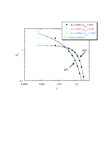
Figure 3: The $q_{L}(y)$ curves calculated for the $\pi/2$ and $\pi/4$ wedges and for the values of the parameters $q_{0}=1$, $\alpha_{L}=1$ and $t=0.01$. The results of the numerical solution by BEM (to be compared with the exact analytical solution) are presented for the different time and space discretization parameters.

The results for $\theta=\pi/4$ and $\pi/2$ are shown in Fig. 3 to be compared with the solid curves calculated using (17) and its analog for $\theta=\pi/2$ (Eq. 8 from [14]). It is easy to see that the method produces excellent results even for coarse discretization, except for the element closest to the contact point. The algorithm overestimates the value of $q_{L}$ at this element. The error is larger for the $\pi/2$ wedge, for which $q_{L}\rightarrow\infty$ at the contact point. Fig. 3 demonstrates that the increase of the numerical error with the increase of the time and space steps is very weak.

4 Numerical implementation

Since we chose $\psi$ and $\zeta$ to be zero at infinity, (38) is satisfied trivially on the semicircles of the infinite radius that close the contours $\partial\Omega_{L}$ and $\partial\Omega_{S}$. Thus these circles can be excluded. Then $\partial\Omega_{L}=\partial\Omega_{i}\cup\partial\Omega_{w}$ and $\partial\Omega_{S}=\partial\Omega_{d}\cup\partial\Omega_{w}$. The direction of the unit normal vector $\vec{n}$ is chosen to be external to $\Omega_{L}$ in the following, see Fig. 1. Then it is internal to $\Omega_{S}$, which requires the sign of the integral over $\partial\Omega_{S}$ to be changed. Making use of the boundary conditions (33 – 35), the system of Eqs. 38 reduces to

$$\int\limits_{0}^{t_{F}}{\rm d}t\Biggl{\{}\;\int\limits_{(\partial\Omega_{i})}\left[G^{L}\left({\rm Fo}_{L}{\zeta_{L}\over k_{L}}-T_{inf}v^{n}\right)+{\rm Fo}_{L}T_{inf}{\partial G^{L}\over\partial\vec{n}}\right]{\rm d}\partial\Omega+$$

$${\rm Fo}_{L}\int\limits_{(\partial\Omega_{w})}\left(G^{L}{\zeta_{S}\over k_{L}}-\psi_{S}{\partial G^{L}\over\partial\vec{n}}\right){\rm d}\partial\Omega\Biggr{\}}={1\over 2}\left\{\begin{array}[]{ll}\psi_{S},&\vec{r}_{F}\in\partial\Omega_{w},\\ -T_{inf},&\vec{r}_{F}\in\partial\Omega_{i},\end{array}\right.,$$ (45)

$${\rm Fo}_{S}\int\limits_{0}^{t_{F}}{\rm d}t\Biggl{[}\;\int\limits_{(\partial\Omega_{w})}\left(-G^{S}{\zeta_{S}\over k_{S}}+\psi_{S}{\partial G^{S}\over\partial\vec{n}}\right){\rm d}\partial\Omega+$$

$$\int\limits_{(\partial\Omega_{d})}\left(G^{S}{q_{0}\over k_{S}}+\psi_{S}{\partial G^{S}\over\partial\vec{n}}\right){\rm d}\partial\Omega\Biggr{]}={1\over 2}\psi_{S},\quad\vec{r}_{F}\in\partial\Omega_{d}\cup\partial\Omega_{w},$$ (46)

where the arguments of all functions are supposed to be exactly as in (38). These equations should be solved using the BEM described in the previous section for unknown functions $\zeta_{L}(\vec{r},t)$ for $\vec{r}\in\partial\Omega_{i}$, $\psi_{S}(\vec{r},t)$ for $\vec{r}\in\partial\Omega_{d}\cup\partial\Omega_{w}$, and $\zeta_{S}(\vec{r},t)$ for $\vec{r}\in\partial\Omega_{w}$.

The discretization of the integration subcontours $\partial\Omega_{w}$, $\partial\Omega_{d}$ and $\partial\Omega_{i}$ follows the same exponential scheme (see Fig. 1) that was used for the discretization of the wedge sides in the test example above. The only difference is the axial symmetry of the mesh that corresponds to the symmetry of the bubble. Since the free boundary introduces a nonlinearity into the problem, the following iteration algorithm is needed to determine the bubble shape on each time step [21]:

1. Shape of the bubble is guessed to be the same as on the previous time step;

2. The variations of $v^{n}$ and $P_{r}$ along the bubble interface are guessed to be the same as on the previous time step;

3. Discretization of the contours $\partial\Omega_{w}$, $\partial\Omega_{d}$ and $\partial\Omega_{i}$ is performed;

4. Temperatures and fluxes on the contours $\partial\Omega_{w}$, $\partial\Omega_{d}$ and $\partial\Omega_{i}$ are found using the described above BEM techniques;

5. Volume $V$ and vapor recoil $P_{r}$ are calculated using (36) and (37);

6. Bubble shape is determined (see Sec. 2) for the calculated values of $V$ and $P_{r}$;

7. If the calculated shape differs too much from that on the previous iteration, the velocity of interface $v^{n}$ is calculated, and steps 3 – 7 are repeated until the required accuracy is attained.

As a rule, three iterations give the 0.1% accuracy which is sufficient for our purposes.

The normal velocity of interface $v^{n}_{Fi}$ at the time $F$ and at node $i$ is calculated using the expression

$$v^{n}_{Fi}=(x_{Fi}-x_{(F-1)j})n^{x}_{(F-1)j}+(y_{Fi}-y_{(F-1)j})n^{y}_{(F-1)j},$$ (47)

where $x_{Fi}$ is the coordinate of the node $i$ at time $F$, and $j$ is the number of the node (at time $F-1$) geometrically closest to $(x_{Fi},y_{Fi})$.

The system of Eqs. 5 – 7 is solved by direct integration. The integration of the right-hand side of (7) is performed using the simple mid-point rule, because the values of $P_{r}$ are calculated at the mid-points (nodes) only. The subsequent integration of the right-hand sides of Eqs. 5 – 6 is performed using the Simpson rule (to gain accuracy) for the non-equal intervals. The trapezoidal rule turns out to be accurate enough for the calculation of volume in (4). For the simulation we used the parameters for water at 10 MPa pressure on the heater made of stainless steel (Table 1).

The above described algorithm should give good results when $\int_{0}^{1}P_{r}(\xi){\rm d}\xi$ exists (cf. Eq. 9). In our case $P_{r}(\xi)$ can be approximated by the power function $(1-\xi)^{-2\beta}$ when $\xi\rightarrow 1$. The exponent $\beta$, which comes from the approximation for $q_{L}(\xi)$, turns out to be larger than one half (see discussion in the next section). Thus if the data were extrapolated to the contact point $\xi=1$, this integral would diverge. It is well known, however, that the evaporation heat flux is limited [8] by a flux $q_{max}$. As calculated in the kinetic theory of gases

$$q_{max}=0.74\rho_{V}H\sqrt{R_{g}T_{sat}/(2\pi M)}\approx 10^{4}\mbox{ MW/m}^{2}.$$ (48)

In our model the above divergence appears because of the assumption that the temperature remains constant along the vapor-liquid interface. In reality, this assumption is violated in the very close vicinity of the contact point where the heat flux $q_{L}$ is comparable to $q_{max}$. Thus we accept the following approximation for the function $q_{L}(\xi)$, $\xi<1$. It is extrapolated using the power law $q_{L}(\xi)\propto(1-\xi)^{-\beta}$ until it reaches the value of $q_{max}$ and remains constant while $\xi$ increases to unity. This extrapolation is used to calculate the integrals in (36) and (37). There is no need to modify the constant-temperature boundary condition for the heat transfer calculations because the calculated heat flux $q_{L}$ remains always less than $q_{max}$.

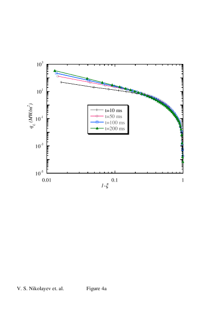
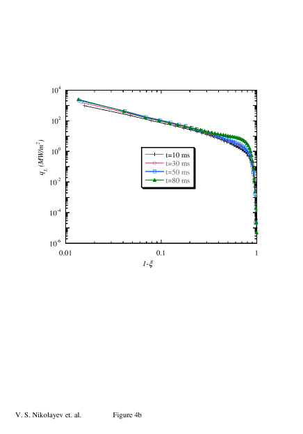
Figure 4: Variation of the heat flux $q_{L}$ (defined in (16)) along the bubble contour for different moments of time. The curvilinear coordinate $\xi$ varies along the bubble contour; $\xi=1$ at the contact point: a) $q_{0}=0.05$ MW/m², b) $q_{0}=0.5$ MW/m².

The calculations show that the function $q_{L}(\xi)$ (see Fig. 4) can be described well by the above power law where $\beta\sim 1$ grows slightly with time. We note that for the growing bubble the divergence is stronger than for the $90^{\circ}$ wedge analyzed in [14]. The difference between these two cases is the behavior of the heat flux $q_{S}$ in the vicinity of the contact point. While it was supposed to be uniform for the $90^{\circ}$ wedge, the function $q_{S}(x)$ increases strongly near the contact point for the growing bubble case, see the discussion associated with Fig. 9.

Sometimes, an occasional “bump” on the $q_{L}(\xi)$ curve appears during the iteration of the steps 3–7 of the algorithm because of inaccurate calculation of the bubble shape when the automatically chosen number of the boundary elements in the vicinity of the contact line is too small. This bump disappears during at most three time steps. This disappearance indicates a good numerical stability of the algorithm. When the bubble evolution is exceedingly slow, it may be necessary to increase the time step several times. While not influencing accuracy strongly (this is an intrinsic property of the BEM [22]), such a change decreases the temporal resolution.

5 Results and discussion

There is a number of new results that we have obtained from this simulation. The most important is the time evolution of the dry spot under the vapor bubble. At low heat flux, the shape of the bubble stays nearly spherical (Fig. 5a) until it leaves the heating surface under the action of gravity or hydrodynamic drag forces. Fig. 5b shows that at large heat flux the radius of the dry spot can approach the bubble radius during its evolution, thus confirming previous theoretical predictions [14] where the apparent contact angle grow with time. It should be emphasized that the actual contact angle remains zero during the evolution, see sec. 2. The large apparent contact angle is due to the strong change in slope of the bubble contour near the contact line where the vapor recoil force is very large (see [14] for the advanced discussion). The temporal evolution of the radius $R_{d}$ of the dry spot is illustrated in Fig. 6, where the time evolution of $R_{d}/R$ is shown. $R$ is the visible bubble radius defined as the maximum abscissa for the points of the bubble contour as shown in Fig. 1. Note that $R_{d}/R\leq 1$ by definition. At low heat fluxes $q_{0}<100$ kW/m² $R_{d}$ stays very small during a long time interval (see Fig. 5a). In this regime the bubble should leave the heater quickly because of the small adhesion that is proportional to the contact line length. After a transition time $t_{c}$ which depends on $q_{0}$, the growth of the dry spot accelerates steeply (see Fig. 6). This time $t_{c}$ corresponds to the moment where the growing vapor recoil force becomes comparable to the surface tension. This force balance was analyzed in details in [14], where numerical estimates were given. The dependence $t_{c}(q_{0})$ is presented in Fig. 7. Clearly, $t_{c}$ is a decreasing function of $q_{0}$. This means that, at a sufficiently large $q_{0}$, the dry spot becomes very large in a short time and the departure of the bubble is prevented because of the large adhesion to the heater. During the further growth this bubble can either create alone a nucleus for the film boiling or coalesce with another similarly spreading neighboring bubble. Therefore, we can associate this value of $q_{0}$ with the $q_{CHF}$. Without a careful analysis of the time of departure, it is not possible to determine a precise value for $q_{CHF}$. This will be the subject of future studies.

We neglected the initial superheating for the sake of simplicity. The initial superheating would accelerate the bubble growth slightly in the initial stages that are not important for the dry spot spreading that becomes significant later on.

Slight oscillations in the dry spot growth are clearly visible in Fig. 6, especially in the fast growth regime. We varied the numerical discretization parameters in order to check whether these oscillations appear due to a numerical instability. Neither the amplitude nor frequency of the oscillations depends on numerical discretization parameters. We conclude that the oscillations reflect a physical effect (see below) rather than a numerical artifact.

The kinetics of the bubble growth is illustrated in Fig. 8, where the temporal evolution of the bubble radius $R$ is presented. At $t<t_{c}$ we recover a general tendency of the bubble growth curves (see, e. g. [2, 3]), where $R\propto t^{1/2}$. At $t>t_{c}$ the growth exponent is larger. The curve $R(t)$ exhibits oscillations with their amplitude increasing with time. We suspect that this effect appears when the temperature distribution in the heater responds too slowly to maintain the fast growth rate in the bubble.

Our simulation enables the heat transfer under the bubble to be rigorously calculated. The variation of the heat flux $q_{S}$ along the heating surface is shown in Figs. 9a,b for the different values of the heat flux $q_{0}$. The value of $q_{S}$ on the liquid side in the vicinity of the contact line turns out to be very close to $q_{L}$, the heat flux that produces evaporation on the vapor-liquid interface and that diverges on the contact line (see Figs. 4). This correspondence was expected, because all the heat flux supplied by the heater to the foot of the bubble is consummated to evaporate the liquid, in agreement with the “liquid microlayer” models. Since $q_{S}$ is zero (cf. (23)) if the contact line is approached from the dry spot side, the function $q_{S}(x)$ is discontinuous in the vicinity of the contact point. Far from the bubble $q_{S}=q_{0}$ as it should be.

The variation of the temperature along the heating surface $T_{S}(x)$ is also shown in Figs. 9. Far from the bubble, $T_{S}$ has to increase with time independently of $x$ and follows a square root law according to (29). It decreases to $T_{sat}$ near the contact point because the temperature should be equal to $T_{sat}$ on the whole vapor-liquid interface, according to the imposed boundary condition. Figs. 9 demonstrate that there is a zone of lowered temperature around the bubble, in agreement with the experimental observations [2]. Inside the dry spot, $T_{S}$ increases with time sharply because the heat transfer through the dry spot is blocked. Fig. 9b shows that at high heat flux and $t>t_{c}$ the temperature inside the dry spot becomes larger than the temperature far from the bubble. This temperature increase leads to eventual burnout of the heater observed during the boiling crisis. The presence of singularities in the functions $T_{S}(x)$ and $q_{S}(x)$ is the reason for our choice of the boundary conditions on the heating surface in the form (23,24). As a matter of fact, an application of the conditions of the uniform heat flux or uniform temperature would lead to the physically inconsistent results such as non-integrable divergency of $q_{L}$ at the contact line. We note that an error in the calculation of $q_{L}$ should strongly influence the results for the dry spot dynamics.

6 Conclusions

The 2D free-boundary simulation allows us to calculate the actual bubble shape and the variation of the temperatures and fluxes along the vapor-liquid, vapor-solid, and liquid-solid interfaces. The description of the heat transfer in the vicinity of the triple contact line presents the most difficult part of the problem. Our variation of the Boundary Element Method is capable of adequately describing it.

Our main result is the evidence for the growth of the dry spot under the vapor bubble. While this increase is very slow in the beginning of the bubble growth, it accelerates steeply after a growth time $t_{c}$ that depends on the external heat supply. At low heat supply, $t_{c}$ is very large so that the bubble can grow large enough to satisfy the conditions for departure from the heating surface before the dry spot becomes significant. In contrast, at high heat supply, $t_{c}$ is small so that the dry spot grows very rapidly which means that the bubble spreads over the heating surface. Although our analysis is limited to the case of high system pressures, we note that at low pressures this effect can also be important because the forces of dynamical origin “press” the bubble against the heater, thus favoring its spreading. The results of this simulations thus confirm the validity of the “drying transition” model suggested in [14] to describe the boiling crisis.

Unfortunately, observations of the bubble shape and the dry spot growth during boiling at high pressures and high heat fluxes are unknown to us, preventing a direct comparison of our results with the experimental data. We note, however, that the growth of the dry spot immediately before the boiling crisis was observed in [9, 10], where observations have been carried out through a transparent heating surface. The authors of [10] state that “When the heat flux is sufficiently large, suddenly at some point on the heating surface a dry area is not wetted and starts growing, leading to burnout”. This observation confirms directly the validity of our model.

Acknowledgments

The authors would like to acknowledge the financial support of EDF (V. N. and D. B.) and NASA (V. N. and J. H.). This work has been done when one of the authors (V. N.) stayed at the Department of Physics of the UNO, which he would like to thank for its kind hospitality. V. N. thanks Dr. Hervé Lemonnier for the introduction into the BEM for the heat diffusion. The authors are grateful to Jean-Marc Delhaye for fruitful discussions.

Description	Notation	Value	Units
Saturation temperature	$T_{sat}$	311	∘C
Thermal conductivity of liquid	$k_{L}$	0.55	W/(m K)
Specific heat of liquid	$c_{pL}$	6.12	J/(g K)
Mass density of liquid	$\rho_{L}$	688.63	kg/m3
Mass density of vapor	$\rho_{V}$	55.48	kg/m3
Latent heat of vaporization	$H$	1.3	MJ/kg
Surface tension	$\sigma$	12.04	mN/m
Thermal conductivity of steel	$k_{S}$	15	W/(m K)
Specific heat of steel	—	0.5	J/(g K)
Mass density of steel	—	8000	kg/m3
Initial bubble radius	$R_{0}$	0.05	mm
Reference heat flux	$\bar{q}$	1	MW/m2
Reference thermal conductivity	$\bar{k}$	1	W/(m K)
Minimal discretization step	$d_{min}$	0.001	$R_{0}$
Time step	$\Delta t$	1	ms

Table 1: Values of parameters used in the simulation.

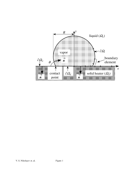
Figure 1: Vapor bubble on the heating surface surrounded by liquid. The chosen direction of the unit normal vector $\vec{n}$ is shown for each of the subcontours $\partial\Omega_{w}$, $\partial\Omega_{d}$ and $\partial\Omega_{i}$. The discretization is illustrated for the right half of the subcontours.

Figure 5: The bubble shape shown for the different growth times. a)$q_{0}=0.05$ MW/m²; b) $q_{0}=0.5$ MW/m²;

Figure 6: The temporal evolution of the quotient of the dry spot radius $R_{d}$ and the bubble radius $R$ for different values of $q_{0}$ expressed in MW/m². $R$ is measured as shown in Fig. 1. The transition time $t_{c}$ is shown for $q_{0}=0.05$ MW/m².

Figure 7: The transition time $t_{c}$ as a function of the heat flux $q_{0}$.

Figure 8: Temporal evolution of the bubble radius $R$ for different values of $q_{0}$ expressed in MW/m². $R$ is measured as shown in Fig. 1.

Figure 9: Variation of the heat flux $q_{S}$ and the temperature $T_{S}$ along the surface of the heater for a)$q_{0}=0.05$ MW/m², $t=200$ ms; b)$q_{0}=0.5$ MW/m², $t=80$ ms. The point $x=0$ corresponds to the center of the bubble. $T_{S}-T_{sat}=0$ at the contact point, $q_{S}=0$ to the left of it, i.e. inside the dry spot.

Appendix A Volume determination

The volume $V$ of an object $\Omega$ can be calculated as

$$V=\int\limits_{(\Omega)}{\rm d}\Omega={1\over 2}\int\limits_{(\Omega)}\mbox{div}(x\vec{e}_{x}+y\vec{e}_{y})\;{\rm d}\Omega,$$ (49)

using the obvious equality

$$\mbox{div}(x\vec{e}_{x}+y\vec{e}_{y})=2,$$

where $\vec{e}_{x}=(1,0)$ and $\vec{e}_{y}=(0,1)$ are the unit vectors directed along the axes. The Gauss integral theorem is valid for any $\vec{a}$ and $\Omega$:

$$\int\limits_{(\Omega)}\mbox{div}\vec{a}\;{\rm d}\Omega=\int\limits_{(\partial\Omega)}\vec{a}\cdot\vec{n}_{e}\;{\rm d}\,\partial\Omega,$$ (50)

where $\partial\Omega$ denotes the surface of $\Omega$, and $\vec{n}_{e}$ is the external unit normal vector to this surface. In our case $\partial\Omega=\partial\Omega_{i}\cup\partial\Omega_{d}$, where $\partial\Omega_{d}$ is the surface of the vapor-solid contact, i.e. the dry spot. The application of the equality (50) to the last integral in (49) yields the expression

$$V={1\over 2}\int\limits_{(\partial\Omega_{i}\cup\partial\Omega_{d})}(xn_{e}^{x}+yn_{e}^{y})\;{\rm d}\,\partial\Omega.$$ (51)

Since $y=n_{e}^{x}=0$ on $\partial\Omega_{d}$ (see Fig. 1), the integral over it is equal to zero. Thus (51) reduces to (4).

References

- [1] L. S. Tong, Boiling Heat Transfer and Two- Phase Flow (2nd Edn), Taylor & Francis, New York (1997).
- [2] M. G. Cooper, A. J. P. Lloyd, The microlayer in nucleate pool boiling, Int. J. Heat Mass Transfer 12, 895–913 (1969).
- [3] P. Stephan & J. Hammer, A new model for nucleate boiling heat transfer, Wärme- und Stoffübertrangung 30, 119–125 (1985).
- [4] R. C. Lee, J. E. Nydahl, Numerical calculation of bubble growth in nucleate boiling from inception through departure, J. Heat Transfer/Trans. ASME 111, 474–478 (1989).
- [5] R. Mei, W. Chen & J.F. Klausner, Vapor bubbles growth in heterogeneous boiling, Int. J. Heat Mass Transfer 38, 909–919 (1995).
- [6] V. K. Dhir, D. M. Qiu, N. Ramanujapu & M. M.Hasan, Investigation of nucleate boiling mechanisms under microgravity conditions, Proc. IVth Microgravity Fluid Physics & Transport Phenomena Conf., Cleveland, (NASA Publication in the form of Compact Disk, available also from http://www.ncmr.org/events/fluids1998/papers/459.pdf), 435–440 (1998).
- [7] Yu. A. Buyevich, Towards a Unified Theory of Pool Boiling — the Case of Ideally Smooth Heated Wall, Int. J. Fluid Mech. Res., 26(2), p.189–223 (1999).
- [8] van P. Carey, Liquid-Vapor Phase Change Phenomena, Hemisphere, Washington D.C. (1992).
- [9] H. J. van Ouwerkerk, Burnout in pool boiling: the stability of boiling mechanisms, Int. J. Heat Mass Transfer 15, 25–34 (1972).
- [10] K. Torikai, M. Hori, M. Akiyama, T. Kobori & H. Adachi, Boiling Transfer and burn-out mechanism in boiling-water cooled reactors. In: Proc. 3rd UN Int. Conf. Peaceful Uses of Atomic Energy (Geneva, Aug. 31 – Sept. 9, 1964) United Nations, New York, 8, p.146-155 (1964); K. Torikai, K. Suzuki & M. Yamaguchi, Study on Contact Area of Pool Boiling Bubbles on a Heating Surface (Observation of Bubbles in Transition Boiling), JSME Int. J. Series II 34, 195–199 (1991); K. Torikai, K. Suzuki, T. Inoue & T. Shirakawa, Effects of Microlayer and Behavior of Coalesced Bubbles in Transition Boiling for Heat Transfer. In: Heat Transfer: Proc. 3rd UK National Conf. Inc. 1st Eur. Conf. Therm.Sci., p.599-605, Birmingham (1992).
- [11] A. K. Chesters, Modes of bubble growth in the slow-formation regime of nucleate pool boiling, Int. J. Multiphase Flow 4, 279–302 (1978).
- [12] M. A. Johnston, J. de la Pena & R. B. Mesler, Bubble shapes in nucleate boiling, AIChE J. 12, 344 (1966).
- [13] P. Bricard, P. Péturaud & J.-M. Delhaye, Understanding and modeling DNB in forced convective boiling: Modeling of a mechanism based on nucleation site dryout, Multiphase Sci. Techn. 9, No. 4, 329–379 (1997).
- [14] V. S. Nikolayev & D. A. Beysens, Boiling crisis and non-equilibrium drying transition, Europhysics Letters 47, 345–351 (1999).
- [15] H. L. G. Pina & J. L. M. Fernandes, Applications in Transient Heat Conduction. In Topics in Boundary Element Research, Vol.1, Basic Principles and Applications (Edited by C. A. Brebbia), Springer-Verlag, Berlin, pp. 41–58 (1984).
- [16] D. Juric & G. Tryggvason, Computations of Boiling Flows, Int. J. Multiphase Flow 24, 387–410 (1998).
- [17] A. Mazouzi, Etude thermique et hydrodynamique de la croissance des bulles de vapeur en ébullition nucléée. Thèse de l’Université P. et M. Curie, Paris (1995).
- [18] A. Prosperetti & M. S. Plesset, The stability of an evaporating liquid surface, Phys. Fluids 27, 1590–1601 (1984).
- [19] H. S. Carslaw & J. C. Jaeger Conduction of Heat in Solids (2nd Edn), University Press, Oxford (1959).
- [20] Handbook of Mathematical Functions, Eds. M. Abramovitz & I. A. Stegun, Dover, New York (1972).
- [21] W. DeLima-Silva & L. C. Wrobel, A front-tracking BEM formulation for one-phase solidification/melting problems, Engineering Analysis with Boundary Elements 16, 171–182 (1995).
- [22] G.-L. Lagier, Application de la méthode des élements de frontière à la résolution de problèmes de thermique inverse multidimensionnels (Application of the Boundary Element method to multidimensional inverse heat conduction problems), Thése de l’Institut National Polytechnique de Grenoble, Grenoble (1999).
- [23] V. Demirel & S. Wang, An efficient boundary element method for two-dimensional transient wave-propagation problems, Appl. Math. Modeling 11, 411–416 (1987).