New hydrodynamic mechanism for drop coarsening

Abstract

We discuss a new mechanism of drop coarsening due to coalescence only, which describes the late stages of phase separation in fluids. Depending on the volume fraction of the minority phase, we identify two different regimes of growth, where the drops are interconnected and their characteristic size grows linearly with time and where the spherical drops are disconnected and the growth follows (time)^1/3. The transition between the two regimes is sharp and occurs at a well defined volume fraction of order 30%.

In this Letter we concentrate on the kinetics of the late stages of the phase separation. This subject has received considerable attention recently Jaya –Tanaka . Most of the experiments on growth kinetics have been performed near the critical point of binary liquid mixtures (or simple fluids) because there the critical slowing down allows the phenomenon to be observed during a reasonable time. After a thermal quench from the one-phase region to the two-phase region of the phase diagram (Fig. 1) the domains of the new phases nucleate and grow. It turns out that two alternative regimes of coarsening are possible. The first can be observed when the volume fraction $\phi$ of the minority phase is lower than some threshold Knob and the domains of the characteristic size $R$ grow according to the law $R\propto t^{1/3}$ ($t$ is the time elapsed after the quench) as spherical drops. The second regime manifests itself when the quench is performed at high volume fraction, the coarsening law is $R\propto t^{1}$ and the domains grow as a complicated interconnected structure. Recent experiments Perrot show that when $0.1<\phi<0.3$ the $t^{1/3}$ growth can be explained by a mechanism of Brownian drop motion and coalescence rather than the Lifshitz-Slyozov mechanism Lifsh which holds for $\phi\rightarrow 0$ and which we will not discuss here. We are interested in the late stages of growth when phase boundaries are already well developed and the concentrations of the phases are very close to the equilibrium values at given temperature $T$ as defined by the coexistence curve (Fig. 1). Then the drops grow just because the system tends to minimize the total surface separating the phases (i.e. due to coalescence) and $\phi$ no longer depends on time.

Brownian coalescence. The Brownian mechanism was considered first by Smoluchowski Smo for coagulation of colloids and was then applied to phase separation by Binder and Stauffer Binder and Siggia Sig . According to this mechanism, the rate of collisions per unit volume due to the Brownian motion of spherical drops in the liquid of shear viscosity $\eta$ is

$$N_{B}=16\pi DRn^{2}f(\phi),$$ (1)

where $n$ is an average number of drops per volume, $R$ is the average radius of the drops and $D$ is the diffusion coefficient of the drops of the same viscosity

$$D={k_{B}T\over 5\pi\eta R}\quad.$$ (2)

The factor $f$ represents the correction which takes into account the hydrodynamic interaction between the drops. It depends on the ratio of the viscosities of the liquid inside and outside the drops and the average distance between the drops and, therefore, on the volume fraction $\phi$. This correction has been calculated in the dilute limit ($\phi\rightarrow 0$) by Zhang and Davis Zhang . In the proximity of the critical point we can assume the viscosities of the phases to be equal and

$$f(0)=0.56.$$ (3)

According to the model, the drops coalesce immediately after the collision. Coalescence is the only reason for the decrease of the total number of the drops with the rate

$${dn\over dt}=-N_{B}.$$ (4)

With the relation

$$\phi={4\over 3}\pi R^{3}n=\mbox{const},$$ (5)

Eq.(4) yields a $R\propto t^{1/3}$ law. The further improvements (see Hay and refs. therein) of this model influence mainly the numerical factor in (1) which is not important for the present considerations.

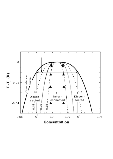
Figure 1: Coexistence curve for a model two-phase system (density-matched cyclohexane–methanol) from Ref. Jaya . The dotted curve is the calculated boundary (see text) between the $t^{1/3}$ and $t^{1}$ growth regions which corresponds to $\phi=0.26$. The triangles are the experimental data from Ref. 1. The curves corresponding to $\phi=0.15$ (random percolation limit) and $\phi=0.35$ (the value which gives the best fit to the experimental data from Ref. 1) are presented also for comparison. The volume fraction of the minority phase at the point $(c,T)$ can be calculated as $\phi=1/2-|c-c_{c}|/(c^{-}-c^{+})$ where $c_{c}$ (=0.707 for this case) is the critical concentration.

Hydrodynamic approaches. The origin of the $R\propto t^{1}$ growth law, observed at high volume fraction where domains are interconnected, is much less clear. By means of a dimensional analysis Siggia Sig has shown that hydrodynamics is needed to explain the kinetics. It assumed the growth to be ruled by the Taylor instability of the long tube of fluid, which breaks into separate drops and associated the growth rate with the rate of the evolution of the unstable fluctuations. This idea has been developed by San Miguel et al. in SanMig . However, it was not clear how this process was related to the growth.

Another approach has been considered by Kawasaki and Ohta Kaw who used a model of coupled equations of hydrodynamics and diffusion. It was assumed that the growth is controlled by diffusion and the hydrodynamic correction to this process was calculated. However, the translational movement of the drops due to the pressure gradient was not taken into account. The motion of the liquid was supposed to be induced by the concentration gradient only. At the same time, it is well known that the concentration variation does not enter the equations of hydrodynamics of the liquid mixture in a first approximation Land . Moreover, it is evident that at high volume fraction the coalescence process induced by the translational motion of the drops becomes very important.

Recently, several groups puri ; alex ; valls ; shino ; appert performed large scale direct numerical simulations by using different approaches to solve coupled equations of diffusion and hydrodynamics. Some recovered the linear growth law alex ; shino , whilst the others were not able to reach the late stages of separation and measured the transient values of the growth exponent (between 1/3 and 1). In spite of these efforts, the physical mechanism for the linear growth has not been clarified. To our knowledge, the simulations never showed two asymptotical laws depending on the volume fraction: the exponent is either larger than 1/3 when accounting for hydrodynamics or 1/3 for pure diffusion. Thus the precise threshold in $\phi$ separating the $t^{1}$ and $t^{1/3}$ regimes is not predicted either by any theory or by simulation.

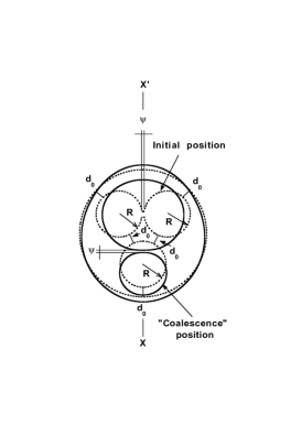
Figure 2: The positions of the drop surfaces at the beginning (dotted line) and at the end (solid line) of the simulation. $\psi$ is the coalescence distance, $d_{0}$ is the initial distance between the drops, $X^{\prime}$–$X$ is the axis of cylindrical symmetry.

Simulation of coalescence. We show here that a $t^{1}$ growth can originate from a coalescence mechanism whose limiting process between two coalescences is not Brownian diffusion but rather flows induced by previous coalescence. We use the concept of “coalescence-induced coalescence” as introduced by Tanaka Tanaka who, however, thought that induction by the hydrodynamic flow was not relevant, having stated that coalescence takes place after the decay of the flow. We consider here a coalescence process between two drops and study numerically the generated flow and its influence on the third neighboring drop. The fully deterministic hydrodynamic problem within the creeping flow approximation (which is well justified near the critical point Sig ) was solved. The free boundary conditions were applied on all drop interfaces whose motion is driven by surface tension. At each time step the velocity of each mesh point on the interface contours was computed using a boundary integral approach Pozdr . When the new positions of the interfaces have been calculated, the procedure was continued iteratively. The details of the solution will be presented elsewhere Prep . We begin the simulation when coalescence starts between two drops of size $R$ (Fig. 2), i.e. when the drops of the minority phase approach to within a distance of coalescence $\psi$ which corresponds to the interface thickness of the drop Sig . We choose for the simulation $R=10\psi$. Then we place another drop at the distance $d_{0}$ from the composite drop (defined as the aggregate of two coalescing drops) and envelope these two drops by a spherical shell to mimic the surrounding pattern of tightly packed drops. Thus the distance between the drops and the shell has been chosen to be $d_{0}$ also. The surface tension $\sigma$ is supposed to be the same for all the interfaces. Unfortunately, due to the prohibitively long computing times, we could not simulate the process of coalescence of two spherical drops. Instead, we had to use a configuration with cylindrical symmetry with respect to the axis $X^{\prime}$ – $X$ (see Fig. 2) which is expected to retain the main features associated with the spherical shape. In the beginning of the simulation the composite drop looks more like a torus. The spherical shell approximation can be justified by the fact that the main effect of the assembly of surrounding drops (as well as of the spherical shell) is to confine the motion of the neighboring drops – see Prep for an advanced discussion. A setup with only two drops without either a shell or surrounding drops would not enable a new coalescence even for the smallest interdrop distances. Though we cannot control quantitatively this approximation, it is the simplest one which captures the main features of the process.

A first important result from the simulation is that the flow generated by the first coalescence is able to generate a second coalescence between the composite drop and the neighboring drop (Fig. 2). This means that the lubrication interaction with the surrounding drops (with the shell in our model) make attract the composite and the neighboring drops (note that the second coalescence does not take place between this neighboring drop and the shell). This leads to the formation of a new elongated droplet. When the drops are close enough to each other the composite drop will have no time to relax to a spherical shape since a new coalescence takes place before relaxation. An interconnected pattern naturally follows. In contrast, when the drops are far from each other ($d_{0}/R\gg 1$), the second coalescence will never take place. The droplets take a spherical shape and the liquid motion stops. It is also clear that if $d_{0}/R<l_{G}$, which we call “geometric coalescence limit”, coalescence necessary occurs due to geometrical constraint. We find $l_{G}\approx 0.484$ Prep , l_G .

The second important result is that the coalescence takes place also for $l_{G}<d_{0}/R<l_{H}$ where $l_{H}$ is a value which we call “hydrodynamic coalescence limit”. It is defined as a reduced initial distance where the time between two coalescences ($t_{c}$) becomes infinite . Since there is only one length scale ($R$) in the problem, $t_{c}$ can be written in the scaled form

$$t_{c}=\alpha\eta R/\sigma,$$ (6)

where $\alpha$ is a reduced coalescence time which depends on $d_{0}/R$ only (Fig. 3).

The quantity $d_{0}/R$ is related to the volume fraction of the drops (minority phase) $\phi$:

$$\phi=b[1+d_{0}/(2R)]^{-3}.$$ (7)

The constant $b$ depends on the space arrangement of the drops. The hydrodynamic interaction between them is always repulsive due to the lubrication force. Thus they tend to be as far from each other as possible. Moreover, experiment shows a liquid-like order for the drop positions. Such a correlation explains why the drops do not percolate Jaya when the volume fraction $\phi$ reaches the random percolation limit $(\phi\approx 0.15)$.

Since no quantitative information is available to determine $b$, we calculate its upper and lower bounds. Ideally, we can assume that the drops are arranged into a regular lattice, with the vertices as far from each other as possible. This is the face centered cubic lattice where $b=\pi/3\sqrt{2}\approx 0.74$ and which corresponds to the fully ordered structure. We can also consider as a lower bound the random close packing arrangement for spheres of radius $R+d_{0}/2$. This corresponds to the absence of a short-range order RP and implies $b\approx 0.64$. We note that the value of $b$ is not very sensitive to the particular space arrangement. In the following we adopt the median value $b=0.69$.

Generalization of the hydrodynamic model. Now we can generalize the above hydrodynamic mechanism for an arbitrary shape of the drops. The self-similarity of the growth implies the following relation for the characteristic sizes of the drops between $i$-th and $(i+1)$-th coalescences: $R^{(i+1)}=\beta R^{(i)}$, where $\beta$ is a universal shape factor, which depends on $\phi$ only. We can rewrite also the Eq. (6) for the time between the coalescences in the form $t_{c}^{(i)}=\alpha(\phi)\eta R^{(i)}/\sigma$, where $\alpha(\phi)$ is also the universal function. The last expression conforms to the scaling assumption which implies the independence of $t_{c}^{(i)}$ on the second length scale $\psi$. Then after $n$ coalescences

$$R=\beta^{n}R^{(0)},\quad t=\sum_{i=0}^{n-1}t_{c}^{(i)}$$

and

$$R=R^{(0)}+{\beta-1\over\alpha}\cdot{\sigma\over\eta}t,$$ (8)

where $R^{(0)}$ is the initial size of the drop. Noting that $\beta=2^{1/3}$ for the spheres and $\beta\gtrsim 1$ for the long tubes, we can take $\beta\sim 1.1$ for the estimate. Since $\alpha\sim 10$ for $\phi=0.5$, as it follows from Fig. 3 and Eq.(7), we obtain $R\sim 0.01\sigma/\eta\,t$, which compares well with the experiment Rate , which gives 0.03 for the numerical factor.

Competition between two mechanisms. Using now Eq. (7) we can relate $l_{H}$ to a volume fraction $\phi_{H}$. It is clear that the described hydrodynamic mechanism works only when $\phi>\phi_{H}$ while the Brownian coalescence takes place in the whole range of $\phi$. Below we shall consider the regime for which $\phi>\phi_{H}$ in order to obtain the position of the boundary between $t^{1/3}$ and $t^{1}$ regions on the phase diagram.

Taking into account the competition between the two mechanisms, we consider the relation

$${dn\over dt}=-(N_{B}+N_{H}),$$ (9)

instead of (4), where $N_{H}$ is the rate of the coalescences due to the hydrodynamics which can be calculated by using Eq.(8) and the relation between $n$ and $R$ (Eq.(5)). The latter, however, depends on the shape of the drop. We assume that in the early stages the drops are spherical and we use Eq.(5). It should be noted that the Eq.(9) rewritten for the scaled wavenumber exactly coincides with the semi-empirical equation suggested by Furukawa Furukawa .

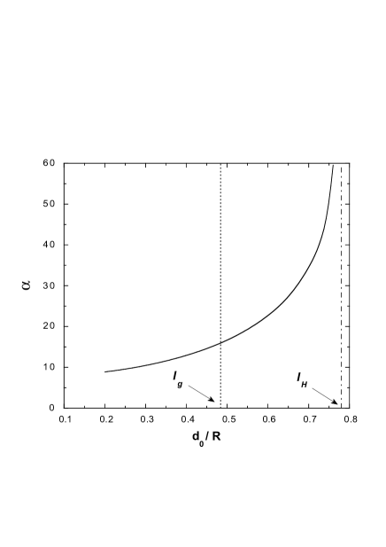
Figure 3: The simulation data on the dependence of the reduced coalescence time $\alpha$ on $d_{0}/R$. The vertical lines show the geometric and hydrodynamic coalescence limits.

The Brownian mechanism dominates when $N_{B}>N_{H}$. In the vicinity of the critical point one can use two-scale-factor universality 2scale expression $\sigma=k_{B}T/\gamma\xi^{2}$ where $\xi$ is the correlation length in the two-phase region, $\gamma\approx 0.39$ is a universal constant. Then we reduce the last inequality to

$$R^{2}/\xi^{2}<G(\phi),$$ (10)

$$\mbox{where}\quad G(\phi)=C\phi f(\phi)\alpha(\phi)\quad\mbox{and}\quad C={\gamma\over 5\pi(\beta-1)}.$$

We do not know much about the function $f(\phi)$ which has been discussed in Eq.(1). However, it is unphysical to assume that it exhibits singularities or a steep behavior. We shall use the constant value (3) in the following. We recall that all our considerations are valid only when the drop interfaces have already formed (late stages of growth), which means that the initial radius of a drop cannot be less than the interface thickness, i. e. $\approx 4\xi$ Thick . It follows readily from the inequality (10) that growth would obey the law $R\propto t^{1/3}$ when

$$G(\phi)>16.$$ (11)

Now we aim to estimate the function $G(\phi)$ by using for $\alpha(\phi)$ the calculated function in Fig. 3 along with Eq.(7). It turns out that the function $G(\phi)$ well fits the power law

$$G(\phi)\propto(\phi-\phi_{H})^{-\delta}$$ (12)

for $\phi>\phi_{H}$ where $\phi_{H}\approx 0.26$, $\delta\approx 0.33$ and the divergency comes from $\alpha(\phi)$. From (12), it is easy to deduce that (11) is valid when $0<\phi-\phi_{H}\lesssim 10^{-6}$. In practice, this means that for all $\phi>\phi_{H}$, the hydrodynamic mechanism only will determine the growth from the very beginning of the drop coarsening. Alternatively, for $\phi<\phi_{H}$, the drops will grow according to the Brownian mechanism only. This explains the sharp transition in the kinetics ($t^{1}\rightarrow t^{1/3}$) which is controlled by the volume fraction of the minority phase as observed in Jaya and Perrot . The curve which corresponds to the threshold value $\phi=0.26$ is plotted in Fig. 1. It shows a reasonable agreement with the experimental data in spite of our very particular choice of the form and arrangement of the drops.

It should be mentioned that our model can be applied to any system where the growth is due to the coalescence of liquid drops inside another fluid (phase separation, coagulation, etc.).

- (1) Y. Jayalakshmi, B. Khalil and D. Beysens, Phys. Rev. Lett. 69, 3088 (1992).
- (2) F. Perrot, P. Guenoun, T. Baumberger, D. Beysens, Y. Garrabos and B. Le Neindre, Phys. Rev. Lett. 73, 688 (1994).
- (3) K. Kawasaki, T. Ohta, Physica A, 118, 175 (1983); T. Koga, K. Kawasaki, M. Takenaka and T. Hashimoto, Physica A, 198, 473 (1993).
- (4) H. Tanaka, Phys. Rev. Lett. 72, 1702 (1994).
- (5) J. D. Gunton, M. San Miguel and P. S. Sahni, in:Phase Transitions and Critical Phenomena, Volume 8, edited by C. Domb and J. L. Lebowitz (New York: Academic Press, 1983), p.267.
- (6) I. M. Lifshitz and V. V. Slyozov, J. Phys.Chem. Solids, 19, 35 (1961).
- (7) M. von Smoluchowski, Z. Phys. Chem. 92, 129 (1917).
- (8) K. Binder and D. Stauffer, Phys. Rev. Lett. 33, 1006 (1974).
- (9) E. D. Siggia, Phys. Rev. A 20, 595 (1979).
- (10) X. Zhang, R. H. Davis, J. Fluid Mech. 230, 479 (1991).
- (11) H. Hayakawa, Physica A 175, 383 (1991).
- (12) M. San Miguel, M. Grant and J. D. Gunton, Phys. Rev. A 31, 1001 (1985).
- (13) L. D. Landau and E. M. Lifshitz, Fluid Mechanics (Pergamon, London, 1959).
- (14) S. Puri and B. Dünweg, Phys. Rev. A 45, R6977 (1992).
- (15) F. J. Alexander, S. Chen, and D. W. Grunau, Phys. Rev. B 48, 634 (1993).
- (16) O. T. Valls and J. E. Farrell. Phys. Rev. E 47, R36 (1993).
- (17) A. Shinozaki and Y. Oono, Phys. Rev. E 48, 2622 (1993).
- (18) C. Appert, J. F. Olson, D. H. Rothman and S. Zaleski, Spinodal decomposition in a three-dimensional, two-phase, hydrodynamic lattice gas, Preprint (1995).
- (19) C. Pozrikidis, Boundary integral and singularity method for linearized viscous flow (Cambridge Univ., Cambridge, 1991).
- (20) V. S. Nikolayev and D. Beysens, ”Coalescence-induced coalescence” by hydrodynamic flow, submitted to J. Fluid Mech. (1996).
- (21) The shell diameter at the initial moment can be defined according to Fig. 2 as a function of , and . If there is no coalescence, the composite drop eventually becomes a sphere with a diameter which can be deduced out of its initial volume, because the latter is conserved during the evolution. The value is determined by the condition which means that two drops of the final spherical shape must fit inside the spherical shell with the gaps of the width .
- (22) J. H. Berryman, Phys. Rev. A 27, 1053 (1983).
- (23) P. Guenoun, R. Gastaud, F. Perrot, D. Beysens, Phys. Rev. A 36, 4876 (1987).
- (24) H. Furukawa, Adv. Phys. 34, 703 (1985).
- (25) M. R. Moldover, Phys. Rev. A 31, 1022 (1985).
- (26) D. Beysens, M. Robert, J. Chem. Phys. 87, 3056 (1987), ibid. 93, 6911 (1990).