Improving bounds for the Perel’man-Pukhov quotient for inner and outer radii

Abstract.

In this work we study upper bounds for the ratio of successive inner and outer radii of a convex body $K$. This problem was studied by Perel’man and Pukhov and it is a natural generalization of the classical results of Jung and Steinhagen. We also introduce a technique which relates sections and projections of a convex body in an optimal way.

1. Introduction

The biggest radius of an $i$-dimensional Euclidean disc contained in an $n$-dimensional convex body $K$ is denoted by $\mathrm{r}_{i}(K)$, whereas the smallest radius of a solid cylinder with $i$-dimensional spherical cross-section containing $K$ is denoted by $\mathrm{R}_{i}(K)$, for any $1\leq i\leq n$. Perel’man in [31] and independently Pukhov in [33] studied the relation between these inner and outer measures, and showed that

(1.1) $$\frac{\mathrm{R}_{n-i+1}(K)}{\mathrm{r}_{i}(K)}\leq i+1,\quad 1\leq i\leq n.$$

Unfortunately, the inequality is far from being best possible. Two remarkable results in Convex Geometry are particular cases of (1.1). Jung’s inquality [28] states

(1.2) $$\frac{\mathrm{R}_{n}(K)}{\mathrm{r}_{1}(K)}\leq\sqrt{\frac{2n}{n+1}},$$

and Steinhagen’s inequality [36] says

(1.3) $$\frac{\mathrm{R}_{1}(K)}{\mathrm{r}_{n}(K)}\leq\left\{\begin{array}[]{ll}\sqrt{n}&\text{if }n\text{ is odd,}\\ \frac{n+1}{\sqrt{n+2}}&\text{if }n\text{ is even.}\end{array}\right.$$

(1.2) and (1.3) are best possible, since the $n$-dimensional regular simplex $\mathrm{S}_{n}$ attains equality in both of them. Therefore, it is natural to conjecture that the regular simplex attains equality in the optimal upper bound for the quotient given in (1.1). If $i=1$ or $i=n$ the simplex $\mathrm{S}_{n}$ attains equality in (1.2) and (1.3). If $i=2$ and $n$ is even, then

$$\frac{\mathrm{R}_{n-1}(\mathrm{S}_{n})}{\mathrm{r}_{2}(\mathrm{S}_{n})}=\frac{(2n-1)\sqrt{3}}{\sqrt{2n(n+1)}},$$

and in the remaining cases (c.f. [8]) it holds that

$$\frac{\mathrm{R}_{n-i+1}(\mathrm{S}_{n})}{\mathrm{r}_{i}(\mathrm{S}_{n})}=\sqrt{1-\frac{i}{n+1}}\sqrt{i(i+1)}.$$

In [2] the authors proved the reverse inequality $\mathrm{r}_{i}(K)\leq\mathrm{R}_{n-i+1}(K)$, with equality for the Euclidean ball, and moreover, Perel’man pointed out in [31] that there exists no constant $C>0$ fulfilling $\mathrm{R}_{j}(K)\leq C\mathrm{r}_{i}(K)$, for any $1\leq i\leq n-1$ and $1\leq j\leq n-i$.

Perel’man improved (1.1) when $n=3$ and $i=2$, by reducing the bound $3$ down to $2.151$. The proof of the result, far from being trivial, shows up hard to understand. In Section 4, we will give a comprehensive proof of this inequality, as it has some interest by itself. The proof will also suggest what kind of results would be desirable to be proven, in order to obtain further improvements of this and other bounds.

Both proofs of (1.1) in [31, 33] contain the hidden result that for a simplex $\mathrm{S}_{n}\subset K$ of maximum volume in an $n$-dimensional convex body $K$, it holds $\mathrm{S}_{n}\subset K\subset x+(n+2)\mathrm{S}_{n}$, where $x$ is the barycenter of $\mathrm{S}_{n}$. This directly bounds the so-called Banach-Mazur distance (c.f. [35]) between $K$ and the class of simplices by $n+2$. This fact has been independently proved in [29].

If $K$ is assumed to be a centrally symmetric set, Pukhov [33] (see also [7]) improved the inequality (1.1), by showing that

(1.4) $$\frac{\mathrm{R}_{n-i+1}(K)}{\mathrm{r}_{i}(K)}\leq\sqrt{\mathrm{e}}\min\{\sqrt{i},\sqrt{n-i+1}\},\quad 1\leq i\leq n,$$

and it is neither best possible. In (1.4) $\mathrm{e}$ means the base of the natural logarithm. In [15], we improved the upper bound when $n=3$ and $i=2$, from $\sqrt{2\mathrm{e}}$ down to $2$, but this inequality is still not best possible. Indeed, it is conjectured that the $n$-dimensional cube $\mathrm{C}_{n}$ and the regular crosspolytope $\mathrm{C}_{n}^{\circ}$ provide the biggest ratio in the inequality (1.4). They fulfill

(1.5) $$\frac{\mathrm{R}_{n-i+1}(\mathrm{C}_{n})}{\mathrm{r}_{i}(\mathrm{C}_{n})}=\frac{\mathrm{R}_{n-i+1}(\mathrm{C}_{n}^{\circ})}{\mathrm{r}_{i}(\mathrm{C}_{n}^{\circ})}=\sqrt{\frac{(n-i+1)i}{n}},\quad 1\leq i\leq n,$$

(see [8] and [14]). Our first theorem, which follows from the main result in Section 2, improves (1.4) in the 3-dimensional case.

Theorem 1.1.

For any centrally symmetric convex body $K\subset\mathbb{R}^{3}$, it holds that

$$\frac{\mathrm{R}_{2}(K)}{\mathrm{r}_{2}(K)}\leq\frac{2\sqrt{2}}{\sqrt{3}}<1.633.$$

In Section 3, we improve inequality (1.1) in some cases. Based on some ideas of Perel’man, we are able to show the following theorem.

Theorem 1.2.

For any convex body $K\subset\mathbb{R}^{n}$, it holds that

(1.6) $$\frac{\mathrm{R}_{n-1}(K)}{\mathrm{r}_{2}(K)}\leq 2\sqrt{2}\sqrt{\frac{n-1}{n}}.$$

Moreover, we establish an improved bound for the case $i=n-1$.

Theorem 1.3.

For any convex body $K\subset\mathbb{R}^{n}$, it holds that

(1.7) $$\frac{\mathrm{R}_{2}(K)}{\mathrm{r}_{n-1}(K)}\leq 2\sqrt{2}\sqrt{n}.$$

This result improves inequality (1.1), providing the right order in the dimension.

The outer radii $\mathrm{R}_{i}(K)$ and the inner radii $\mathrm{r}_{i}(K)$ have been extended to arbitrary Minkowski spaces, i.e., finite dimensional normed spaces (cf. [19]). For the sake of completeness, and although this paper is focused in the Euclidean metric, we add a short section 5 in which we provide a general upper bound for the analogous quotient. Indeed, this bound improves (1.4) in some cases.

For more information on the successive radii, their size for particular bodies as well as computational aspects of these radii we refer to [1, 2, 3, 8, 10, 11, 19, 20, 21]. Their relation with other measures have been studied in [2, 23, 24], their behavior with respect to other binary operations in [13, 17, 16], and their extensions to containers different from the Euclidean ball in [19, 26]. Moreover, quotients of different radii have been studied in [3, 10, 15, 19, 21]. We would like to point out that successive radii are particular cases of the so-called Gelfand and Kolmogorov numbers in Banach Space Theory (cf. [12, 18, 32]), and are widely used in Approximation Theory.

We now establish further notation. Let $\mathcal{K}^{n}$ denote the family of all convex bodies, i.e., compact convex sets, in the $n$-dimensional Euclidean space $\mathbb{R}^{n}$, and we always assume $K\in\mathcal{K}^{n}$. The subset of $\mathcal{K}^{n}$ consisting of all centrally (or $0$-) symmetric convex bodies, i.e., such that if $x=(x_{1},\dots,x_{n})^{\intercal}\in K$ then $-x\in K$, is denoted by $\mathcal{K}^{n}_{0}$. Let $|\,\cdot\,|_{2}$ be the standard Euclidean norm in $\mathbb{R}^{n}$ and $\mathrm{B}_{n}$ be the $n$-dimensional Euclidean unit ball.

The set of all $i$-dimensional linear subspaces of $\mathbb{R}^{n}$ is denoted by $\mathcal{L}^{n}_{i}$. For the sake of brevity we denote by $\mathrm{B}_{i,L}=\mathrm{B}_{n}\cap L$ for any $L\in\mathcal{L}^{n}_{i}$. We denote by $\mathop{\mathrm{missing}}{lin}\nolimits(C)$, $\mathop{\mathrm{missing}}{aff}\nolimits(C)$ and $\mathop{\mathrm{missing}}{conv}\nolimits(S)$, the linear, affine and convex hull of $C$, respectively, and we write $\mathop{\mathrm{missing}}{relbd}\nolimits(C)$ to denote the relative boundary of any $C\subset\mathbb{R}^{n}$. For any $x,y\in\mathbb{R}^{n}$, the line segment with endpoints $x$ and $y$ is denoted by $[x,y]:=\mathop{\mathrm{missing}}{conv}\nolimits(\{x,y\})$ We denote by $L^{\bot}$ and $u^{\bot}$ the orthogonal complement to $L$ and $\mathop{\mathrm{missing}}{lin}\nolimits(\{u\})$, respectively, for any $L\in\mathcal{L}^{n}_{i}$ and $u\in\mathbb{R}^{n}$. By $K|L$ we denote the orthogonal projection of $K$ onto $L$. We use $\mathrm{e}_{i}$ for $i$-th canonical unit vector in $\mathbb{R}^{n}$.

The width in the (unit) direction $u$, the diameter, the minimal width, the circumradius and the inradius of $K$, all measured in the Euclidean distance, are denoted by $\omega(K,u)$, $\mathrm{D}(K)$, $\omega(K)$, $\mathrm{R}(K)$ and $\mathrm{r}(K)$, respectively. For more information on these functionals and their properties we refer to [6, pp. 56–59]. Whenever $K\in\mathcal{K}^{n}$ is contained in an affine subspace $x+L$, with $L\in\mathcal{L}^{n}_{i}$ and $x\in\mathbb{R}^{n}$, we write $f(K;x+L)$ to denote that the functional $f$ has to be evaluated with respect to the subspace $x+L$. With this notation, the outer and inner measures $\mathrm{R}_{i}(K)$ and $\mathrm{r}_{i}(K)$ can be expressed as

(1.8) $$\begin{array}[]{ll}\displaystyle\mathrm{R}_{i}(K)=\min_{L\in\mathcal{L}_{i}^{n}}\mathrm{R}(K|L)&\text{ and }\quad\displaystyle\mathrm{r}_{i}(K)=\max_{L\in\mathcal{L}_{i}^{n}}\max_{x\in L^{\bot}}\mathrm{r}(K\cap(x+L);x+L).\end{array}$$

Slightly modifying the definition of the inner radius $\mathrm{r}_{i}(K)$, we obtain another sequence of interior radii (cf. [2], see also [4]),

$$\widetilde{\mathrm{r}}_{i}(K):=\max_{L\in\mathcal{L}^{n}_{i}}\mathrm{r}(K|L;L).$$

These sequences of inner and outer measures extend the classic radii, namely,

$$\begin{split}\mathrm{R}_{n}(K)&=\mathrm{R}(K),\quad\mathrm{r}_{n}(K)=\widetilde{\mathrm{r}}_{n}(K)=\mathrm{r}(K),\\ \mathrm{R}_{1}(K)&=\frac{\omega(K)}{2},\quad\mathrm{r}_{1}(K)=\widetilde{\mathrm{r}}_{1}(K)=\frac{\mathrm{D}(K)}{2}.\end{split}$$

Moreover, the outer radii are increasing in $i$, whereas both sequences of inner radii are decreasing in $i$, $1\leq i\leq n$. We also have that $\mathrm{r}_{i}(K)\leq\widetilde{\mathrm{r}}_{i}(K)$, and for any $K\in\mathcal{K}^{n}_{0}$ and $1\leq i\leq n$, then

(1.9) $$\frac{\mathrm{R}_{n-i+1}(K)}{\widetilde{\mathrm{r}}_{i}(K)}\leq\sqrt{n-i+1}$$

(see Theorem 1.3 in [15]).

2. Centrally symmetric estimate

We first establish a lemma that will be needed in the proof of Theorem 1.1. This lemma reconstructs the largest disc contained in $K$, knowing in advance that a projection of $K$ in a plane $L$ contains a disc of prescribed radius. The main idea in the proof is to find six points in $K$ (three and their mirrored points in the origin), such that they are all contained in a $2$-dimensional subspace and their orthogonal projection onto $L$ forms a regular hexagon. To do so, we build two sequences of six-tuples of points in $K$, and we find the desired six-tuple as a limit of those sequences of six-tuples, using a Bolzano-type argument.

Lemma 2.1.

Let $K\in\mathcal{K}^{3}_{0}$, $L=\mathop{\mathrm{missing}}{lin}\nolimits(\{\mathrm{e}_{1},\mathrm{e}_{2}\})$ and $\mathrm{r}>0$ be such that $\mathrm{r}B_{2,L}\subset K|L$. Then, there exist a regular hexagon $\mathop{\mathrm{missing}}{conv}\nolimits(\{\pm p_{i}:i=1,2,3\})$ inscribed in $\mathrm{r}B_{2,L}$ and points $\pm q_{i}\in K$, $i=1,2,3$, such that $\pm q_{i}|L=\pm p_{i}$, $i=1,2,3$, and $\dim\mathop{\mathrm{missing}}{conv}\nolimits(\{\pm q_{i}:i=1,2,3\})=2$.

Proof.

For a fixed $u_{1}\in\mathop{\mathrm{missing}}{relbd}\nolimits(\mathrm{r}B_{2,L})$, we consider the regular hexagon inscribed in $\mathrm{r}B_{2,L}$ and having $u_{1}$ as a vertex, and call $\overline{u}_{1},\widetilde{u}_{1}$ the closest vertices to $u_{1}$.

Since $u_{1},\overline{u}_{1},\widetilde{u}_{1}\in K|L$, there exist points $x_{1}^{u},\overline{x}_{1}^{u},\widetilde{x}_{1}^{u}\in K$ such that

$$x_{1}^{u}|L=u_{1},\quad\overline{x}_{1}^{u}|L=\overline{u}_{1}\quad\text{and}\quad\widetilde{x}_{1}^{u}|L=\widetilde{u}_{1}.$$

If $x^{u}_{1}\in\mathop{\mathrm{missing}}{lin}\nolimits(\{\overline{x}^{u}_{1},\widetilde{x}^{u}_{1}\})$, then $\mathop{\mathrm{missing}}{conv}\nolimits(\{\pm x^{u}_{1},\pm\overline{x}^{u}_{1},\pm\widetilde{x}^{u}_{1}\})$ is a 2-dimensional convex body whose projection onto $L$ is the regular hexagon $\mathop{\mathrm{missing}}{conv}\nolimits(\{\pm u_{1},\pm\overline{u}_{1},\pm\widetilde{u}_{1}\})$. In this case, $p_{1}:=u_{1}$, $p_{2}:=\overline{u}_{1}$, $p_{3}:=\widetilde{u}_{1}$, and $q_{1}:=x^{u}_{1}$, $q_{2}:=\overline{x}^{u}_{1}$, $q_{3}:=\widetilde{x}^{u}_{1}$ show the lemma (cf. Figure 1). So, we assume $x^{u}_{1}\notin\mathop{\mathrm{missing}}{lin}\nolimits(\{\overline{x}^{u}_{1},\widetilde{x}^{u}_{1}\})$.

We observe that $x^{u}_{1}\in\mathop{\mathrm{missing}}{lin}\nolimits(\{\overline{x}^{u}_{1},\widetilde{x}^{u}_{1}\})$ if and only if there exist $t,s\in\mathbb{R}$ such that

$$t\bigl{(}\overline{u}_{1},\overline{x}_{13}^{u}\bigr{)}^{\intercal}+s\bigl{(}\widetilde{u}_{1},\widetilde{x}_{13}^{u}\bigr{)}^{\intercal}=t\overline{x}^{u}_{1}+s\widetilde{x}^{u}_{1}=x^{u}_{1}=\bigl{(}u_{1},x^{u}_{13}\bigr{)}^{\intercal},$$

which holds if and only if $t\overline{u}_{1}+s\widetilde{u}_{1}=u_{1}$ and $t\overline{x}^{u}_{13}+s\widetilde{x}^{u}_{13}=x^{u}_{13}$. Since $u_{1},\overline{u}_{1},\widetilde{u}_{1}$ are consecutive vertices of a regular hexagon, the unique solution of $t\overline{u}_{1}+s\widetilde{u}_{1}=u_{1}$ is $t=s=1$. Therefore, $x^{u}_{1}\notin\mathop{\mathrm{missing}}{lin}\nolimits(\{\overline{x}^{u}_{1},\widetilde{x}^{u}_{1}\})$ if and only if $\overline{x}^{u}_{13}+\widetilde{x}^{u}_{13}\neq x^{u}_{13}$. We suppose without loss of generality that $\overline{x}^{u}_{13}+\widetilde{x}^{u}_{13}>x^{u}_{13}$. For the rest of the proof we will use the same notation in the construction of the points, namely: from any point $v\in\mathop{\mathrm{missing}}{relbd}\nolimits(\mathrm{r}B_{2,L})$, we derive $\overline{v}$, $\widetilde{v}$, $x^{v}$, etc.

We write $w_{1}:=-u_{1}$. Then $\overline{w}_{1}=-\overline{u}_{1}$, $\widetilde{w}_{1}=-\widetilde{u}_{1}$ and the symmetry of $K$ imply that $x^{w}_{1}=-x^{u}_{1}$, $\overline{x}^{w}_{1}=-\overline{x}^{u}_{1}$, $\widetilde{x}^{w}_{1}=-\widetilde{x}^{u}_{1}$, and thus

$$\overline{x}^{w}_{13}+\widetilde{x}^{w}_{13}=-\overline{x}^{u}_{13}-\widetilde{x}^{u}_{13}<-x^{u}_{13}=x^{w}_{13}.$$

Let $u_{2}\in\mathop{\mathrm{missing}}{relbd}\nolimits(\mathrm{r}B_{2,L})$ be the “midpoint” on the circumference $\mathop{\mathrm{missing}}{relbd}\nolimits(\mathrm{r}B_{2,L})$ between $u_{1}$ and $w_{1}$. If $x^{u}_{23}=\overline{x}^{u}_{23}+\widetilde{x}^{u}_{23}$ then $p_{1}:=u_{2}$, $p_{2}:=\overline{u}_{2}$, $p_{3}:=\widetilde{u}_{2}$, and $q_{1}:=x^{u}_{2}$, $q_{2}:=\overline{x}^{u}_{2}$, $q_{3}:=\widetilde{x}^{u}_{2}$ show the lemma. If that is not the case, then we can assume that $\overline{x}^{u}_{23}+\widetilde{x}^{u}_{23}>x^{u}_{23}$ and define $w_{2}:=w_{1}$; otherwise we just take $w_{2}$ to be the midpoint and define $u_{2}:=u_{1}$. In the next step we take again the midpoint $u_{3}=(u_{2}+w_{2})/\left|u_{2}+w_{2}\right|_{2}\in\mathop{\mathrm{missing}}{relbd}\nolimits(\mathrm{r}B_{2,L})$ and do the same construction.

Iterating the process, either we find three points $p_{i}$, $i=1,2,3$, verifying the required condition in some step, or we get two sequences $(u_{n})_{n},(w_{n})_{n}\subset\mathop{\mathrm{missing}}{relbd}\nolimits(\mathrm{r}B_{2,L})$, satisfying the following properties:

• $d(u_{n},w_{n})=(1/2)d(u_{n-1},w_{n-1})$, where $d(a,b)$ is the length of the shortest arc in $\mathop{\mathrm{missing}}{relbd}\nolimits(\mathrm{r}B_{2,L})$ joining the points $a,b\in\mathop{\mathrm{missing}}{relbd}\nolimits(\mathrm{r}B_{2,L})$.

• $\lim_{n\rightarrow\infty}u_{n}=\lim_{n\rightarrow\infty}w_{n}\in\mathop{\mathrm{missing}}{relbd}\nolimits(\mathrm{r}B_{2,L})$. Let $p_{1}:=\lim_{n\rightarrow\infty}u_{n}$.

• The vertices of the two corresponding hexagons sequences tend to the appropriate limit, say $\lim_{n\rightarrow\infty}\overline{u}_{n}=\lim_{n\rightarrow\infty}\overline{w}_{n}=:p_{2}$ and $\lim_{n\rightarrow\infty}\widetilde{u}_{n}=\lim_{n\rightarrow\infty}\widetilde{w}_{n}=:p_{3}$.

• $\overline{x}^{u}_{n3}+\widetilde{x}^{u}_{n3}>x^{u}_{n3}$ and $\overline{x}^{w}_{n3}+\widetilde{x}^{w}_{n3}<x^{w}_{n3}$, for all $n\in\mathbb{N}$.

With this process, we also get sequences of points in $K$, namely $(x^{u}_{n})_{n}$, $(\overline{x}^{u}_{n})_{n}$, $(\widetilde{x}^{u}_{n})_{n}$, $(x^{w}_{n})_{n}$, $(\overline{x}^{w}_{n})_{n}$ and $(\widetilde{x}^{w}_{n})_{n}$. Since they are bounded sequences (because they are contained in $K$), there exist convergent subsequences in $K$ and we can suppose without loss of generality that they are the same sequences. Thus

$$\begin{split}\lim_{n\rightarrow\infty}x^{u}_{n}&=x^{u}_{0}\in K,\quad\lim_{n\rightarrow\infty}\overline{x}^{u}_{n}=\overline{x}^{u}_{0}\in K,\quad\lim_{n\rightarrow\infty}\widetilde{x}^{u}_{n}=\widetilde{x}^{u}_{0}\in K,\\ \lim_{n\rightarrow\infty}x^{w}_{n}&=x^{w}_{0}\in K,\quad\lim_{n\rightarrow\infty}\overline{x}^{w}_{n}=\overline{x}^{w}_{0}\in K,\quad\lim_{n\rightarrow\infty}\widetilde{x}^{w}_{n}=\widetilde{x}^{w}_{0}\in K.\end{split}$$

We observe that

$$x^{u}_{0}|L=\left(\lim_{n\rightarrow\infty}x^{u}_{n}\right)|L=\lim_{n\rightarrow\infty}(x^{u}_{n}|L)=\lim_{n\rightarrow\infty}u_{n}=p_{1},$$

and analogously,

$$x^{w}_{0}|L=p_{1},\quad\overline{x}_{0}^{u}|L=\overline{x}^{w}_{0}|L=p_{2}\quad\text{and}\quad\widetilde{x}^{u}_{0}|L=\widetilde{x}^{w}_{0}|L=p_{3}.$$

We notice also that

$$\overline{x}^{u}_{03}+\widetilde{x}^{u}_{03}=\left(\lim_{n\rightarrow\infty}\overline{x}^{u}_{n}\right)_{3}+\left(\lim_{n\rightarrow\infty}\widetilde{x}^{u}_{n}\right)_{3}=\lim_{n\rightarrow\infty}\overline{x}^{u}_{n3}+\lim_{n\rightarrow\infty}\widetilde{x}^{u}_{n3}=\lim_{n\rightarrow\infty}\bigl{(}\overline{x}^{u}_{n3}+\widetilde{x}^{u}_{n3}\bigr{)}\geq\lim_{n\rightarrow\infty}x^{u}_{n3}=x^{u}_{03},$$

and analogously, $\overline{x}^{w}_{03}+\widetilde{x}^{w}_{03}\leq x^{w}_{03}$.

If $\overline{x}^{u}_{03}+\widetilde{x}^{u}_{03}=x^{u}_{03}$ then the set of points $q_{1}:=x_{0}^{u}$, $q_{2}:=\overline{x}_{0}^{u}$, $q_{3}:=\widetilde{x}_{0}^{u}$ together with $p_{1},p_{2},p_{3}$ show the lemma. Otherwise, $\overline{x}^{u}_{03}+\widetilde{x}^{u}_{03}>x^{u}_{03}$. We observe that if $\overline{x}^{w}_{03}+\widetilde{x}^{u}_{03}\leq x^{u}_{03}$ then the lemma is proved: in fact, if this is the case, there exists $\lambda\in[0,1)$ such that

$$\bigl{(}\lambda\overline{x}^{u}_{0}+(1-\lambda)\overline{x}^{w}_{0}\bigr{)}_{3}+\widetilde{x}^{u}_{03}=\lambda\overline{x}^{u}_{03}+(1-\lambda)\overline{x}^{w}_{03}+\widetilde{x}^{u}_{03}=x^{u}_{03},$$

with

$$\lambda\overline{x}^{u}_{0}+(1-\lambda)\overline{x}^{w}_{0}\in K,\quad\bigl{(}\lambda\overline{x}^{u}_{0}+(1-\lambda)\overline{x}^{w}_{0}\bigr{)}|L=\lambda p_{1}+(1-\lambda)p_{1}=p_{1},$$

and thus the set of points $q_{1}:=x^{u}_{0}$, $q_{2}:=\lambda\overline{x}^{u}_{0}+(1-\lambda)\overline{x}^{w}_{0}$, $q_{3}:=\widetilde{x}^{u}_{0}$ shows the lemma.

So we assume that $\overline{x}^{w}_{03}+\widetilde{x}^{u}_{03}>x^{u}_{03}$. Similarly, we now have that if $\overline{x}^{w}_{03}+\widetilde{x}^{w}_{03}\leq x^{u}_{03}$, then there exists $\lambda\in[0,1)$ such that

$$\overline{x}^{w}_{03}+\bigl{(}\lambda\widetilde{x}^{u}_{0}+(1-\lambda)\widetilde{x}^{w}_{0}\bigr{)}_{3}=\overline{x}^{w}_{03}+\lambda\widetilde{x}^{u}_{03}+(1-\lambda)\widetilde{x}^{w}_{03}=x^{u}_{03},$$

and hence the set of points $q_{1}:=x^{u}_{0}$, $q_{2}:=\overline{x}^{w}_{0}$, $q_{3}:=\lambda\widetilde{x}^{u}_{0}+(1-\lambda)\widetilde{x}^{w}_{0}$ shows the lemma.

So we assume once more that this is not the case, i.e., that $\overline{x}^{w}_{03}+\widetilde{x}^{w}_{03}>x^{u}_{03}$. But then, since $\overline{x}^{w}_{03}+\widetilde{x}^{w}_{03}\leq x^{w}_{03}$ there exists $\lambda\in[0,1)$ such that

$$\overline{x}^{w}_{03}+\widetilde{x}^{w}_{03}=\lambda x_{03}^{u}+(1-\lambda)x^{w}_{03}=\bigl{(}\lambda x_{0}^{u}+(1-\lambda)x^{w}_{0}\bigr{)}_{3},$$

and thus the points $q_{1}:=\lambda x_{0}^{u}+(1-\lambda)x^{w}_{0}$, $q_{2}:=\overline{x}^{w}_{0}$, $q_{3}:=\widetilde{x}^{w}_{0}$ show the lemma. ∎

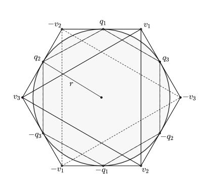
Figure 1. Upper view of the crosspolytope $P_{\varepsilon}:=\mathop{\mathrm{missing}}{conv}\nolimits(\{\pm v_{i}:i=1,2,3\})$, where $v_{1}=(1/\sqrt{3},1,\varepsilon)^{\intercal}$, $v_{2}=(1/\sqrt{3},-1,\varepsilon)^{\intercal}$, $v_{3}=(-2/\sqrt{3},0,\varepsilon)^{\intercal}$, and $\varepsilon>0$. $P_{\varepsilon}$ has a hexagonal central section of vertices $\pm q_{i}$, $i=1,2,3$, and $r\mathrm{B}_{2,\mathrm{e}_{3}^{\bot}}\subset P_{\varepsilon}|\mathrm{e}_{3}^{\bot}$.

Using Lemma 2.1, we derive an inequality relating $\mathrm{r}_{2}(K)$ and $\widetilde{\mathrm{r}}_{2}(K)$ for any $3$-dimensional set.

Theorem 2.1.

Let $K\in\mathcal{K}^{3}_{0}$. Then

$$\frac{\widetilde{\mathrm{r}}_{2}(K)}{\mathrm{r}_{2}(K)}\leq\frac{2}{\sqrt{3}}.$$

The inequality is best possible.

Proof.

By definition of $\widetilde{\mathrm{r}}_{2}(K)$, there exists $L\in\mathcal{L}^{3}_{2}$ such that $\widetilde{\mathrm{r}}_{2}(K)=\mathrm{r}(K|L;L)$. After a suitable rigid motion, we can assume without loss of generality that $L=\mathop{\mathrm{missing}}{lin}\nolimits(\{\mathrm{e}_{1},\mathrm{e}_{2}\})$ and that $\mathrm{r}(K|L;L)B_{2,L}\subset K|L$. We now apply Lemma 2.1 and find an inscribed regular hexagon

$$H=\mathop{\mathrm{missing}}{conv}\nolimits(\{\pm p_{i}:i=1,2,3\})\subset\mathrm{r}(K|L;L)B_{2,L}$$

and points $\pm q_{i}\in K$, $i=1,2,3$, such that

$$\pm q_{i}|L=\pm p_{i},\;i=1,2,3,\quad\text{ and }\quad\dim\mathop{\mathrm{missing}}{conv}\nolimits(\{\pm q_{i}:i=1,2,3\})=2.$$

We call $C=\mathop{\mathrm{missing}}{conv}\nolimits(\{\pm q_{i}:i=1,2,3\})$ and $L^{\prime}=\mathop{\mathrm{missing}}{lin}\nolimits C$. Then,

$$\mathrm{r}_{2}(K)\geq\mathrm{r}(K\cap L^{\prime};L^{\prime})\geq\mathrm{r}(C;L^{\prime}).$$

We now show that $\mathrm{r}(C;L^{\prime})\geq\mathrm{r}(H;L)$. Clearly,

$$\mathrm{r}(C;L^{\prime})=\min_{x\in\mathop{\mathrm{missing}}{relbd}\nolimits C}\left|x\right|_{2}=\left|x_{0}\right|_{2}$$

for some $x_{0}\in\mathop{\mathrm{missing}}{relbd}\nolimits C$. We can suppose that the points $q_{1}$ and $q_{2}$ are consecutive vertices and that $x_{0}=\lambda q_{1}+(1-\lambda)q_{2}$, for some $\lambda\in(0,1)$. Since $q_{j}|L=p_{j}$, we have $q_{j}=(p_{j},q_{j3})^{\intercal}$, $j=1,2$, and then

$$\left|x_{0}\right|^{2}_{2}=\bigl{|}\lambda q_{1}+(1-\lambda)q_{2}\bigr{|}^{2}_{2}=\bigl{|}\lambda p_{1}+(1-\lambda)p_{2}\bigr{|}^{2}_{2}+\bigl{|}\lambda q_{13}+(1-\lambda)q_{23}\bigr{|}^{2}\geq\bigl{|}\lambda p_{1}+(1-\lambda)p_{2}\bigr{|}^{2}_{2}.$$

The point $\lambda p_{1}+(1-\lambda)p_{2}\in\mathop{\mathrm{missing}}{relbd}\nolimits H$, and therefore

$$\bigl{|}\lambda p_{1}+(1-\lambda)p_{2}\bigr{|}_{2}\geq\min_{y\in\mathop{\mathrm{missing}}{relbd}\nolimits H}\left|y\right|_{2}=\mathrm{r}(H;L).$$

From that, we get $\mathrm{r}(C;L^{\prime})=\left|x_{0}\right|_{2}\geq\mathrm{r}(H;L)$ and then

$$\mathrm{r}_{2}(K)\geq\mathrm{r}(C;L^{\prime})\geq\mathrm{r}(H;L)=\frac{\sqrt{3}}{2}\,\widetilde{\mathrm{r}}_{2}(K).$$

It remains to be shown that the inequality is best possible. Let $P_{\varepsilon}=\mathop{\mathrm{missing}}{conv}\nolimits(\{\pm v_{1},\pm v_{2},\pm v_{3}\})$ be the non-regular triangular antiprism in $\mathbb{R}^{3}$ with vertices

$$v_{1}=\left(\frac{1}{\sqrt{3}},1,\varepsilon\right)^{\intercal},\quad v_{2}=\left(\frac{1}{\sqrt{3}},-1,\varepsilon\right)^{\intercal},\quad v_{3}=\left(-\frac{2}{\sqrt{3}},0,\varepsilon\right)^{\intercal},$$

$\varepsilon>0$ (see Figure 1). In pg. 10 and Figure 1 of [17] it was shown that $\mathrm{r}_{2}(P_{\varepsilon})=\sqrt{3}/2$ for $\varepsilon$ small enough. Since the set $P_{\varepsilon}|\mathop{\mathrm{missing}}{lin}\nolimits(\{\mathrm{e}_{1},\mathrm{e}_{2}\})$ is a regular hexagon with $2$-dimensional inradius $1$, then $\widetilde{\mathrm{r}}_{2}(P_{\varepsilon})\geq 1$. Therefore

$$1\leq\widetilde{\mathrm{r}}_{2}(P_{\varepsilon})\leq\frac{2}{\sqrt{3}}\,\mathrm{r}_{2}(P_{\varepsilon})=\frac{2}{\sqrt{3}}\frac{\sqrt{3}}{2}=1,$$

and thus $\widetilde{\mathrm{r}}_{2}(P_{\varepsilon})=(2/\sqrt{3})\,\mathrm{r}_{2}(P_{\varepsilon})$. ∎

Proof of Theorem 1.1.

Particularizing (1.9) in $n=3$ and $i=2$, together with Theorem 2.1, we get that

$$\frac{\mathrm{R}_{2}(K)}{\mathrm{r}_{2}(K)}=\frac{\mathrm{R}_{2}(K)}{\widetilde{\mathrm{r}}_{2}(K)}\frac{\widetilde{\mathrm{r}}_{2}(K)}{\mathrm{r}_{2}(K)}\leq\sqrt{2}\frac{2}{\sqrt{3}}.\qed$$

Before concluding this section, we leave to the reader the analogous statement to Lemma 2.1 and Theorem 2.1 for non-symmetric convex sets.

Lemma 2.2.

Let $K\in\mathcal{K}^{3}$, $L=\mathop{\mathrm{missing}}{lin}\nolimits(\{\mathrm{e}_{1},\mathrm{e}_{2}\})$ and $\mathrm{r}>0$ be such that $\mathrm{r}B_{2,L}\subset K|L$. Then, there exist a square $\mathop{\mathrm{missing}}{conv}\nolimits(\{\pm p_{i}:i=1,2\})$ inscribed in $\mathrm{r}B_{2,L}$ and points $q_{i,\pm}\in K$, $i=1,2$, such that $q_{i,\pm}|L=\pm p_{i}$, $i=1,2$, and $\dim\mathop{\mathrm{missing}}{conv}\nolimits(\{q_{i,\pm}:i=1,2\})=2$.

Theorem 2.2.

Let $K\in\mathcal{K}^{3}$. Then

$$\frac{\widetilde{\mathrm{r}}_{2}(K)}{\mathrm{r}_{2}(K)}\leq\sqrt{2}.$$

The inequality is best possible.

Remark 2.1.

In order to prove Lemma 2.2, it would be sufficient to find an inscribed square, s.t. the segments $[q_{1,+},q_{1,-}]$ and $[q_{2,+},q_{2,-}]$ intersect in their midpoints, i.e., if $(q_{1,+})_{3}+(q_{1,-})_{3}=(q_{2,+})_{3}+(q_{2,-})_{3}$.

Equality holds in Theorem 2.2 for a simplex with vertices

$$\left(\pm 1,0,\varepsilon\right)^{\intercal}\quad\text{and}\quad\left(0,\pm 1,-\varepsilon\right)^{\intercal},$$

for small enough $\varepsilon>0$.

Let us also remark that doing the same as in Theorem 1.1, for $K\in\mathcal{K}^{3}$, i.e. applying Theorem 2.2 and Proposition 2.1 in [15], would imply that

$$\frac{\mathrm{R}_{2}(K)}{\mathrm{r}_{2}(K)}=\frac{\mathrm{R}_{2}(K)}{\widetilde{\mathrm{r}}_{2}(K)}\frac{\widetilde{\mathrm{r}}_{2}(K)}{\mathrm{r}_{2}(K)}\leq 3,$$

still worse than the best known bound 2.151.

3. Improved general upper bounds

In the proof of Theorem 1.2, we extend some ideas of Perel’man [31], slightly modifying some steps.

Proof of Theorem 1.2.

After a suitable translation of $K$, we can suppose that the diameter of $K$ is given by $\mathrm{D}(K)=2\left|p\right|_{2}$ for $p,-p\in K$. Let $p_{1},p_{2}\in K|p^{\bot}$ be such that $\left|p_{1}-p_{2}\right|_{2}=\mathrm{D}(K|p^{\bot})$. We are going to prove that

(3.1) $$\mathrm{D}(K|p^{\bot})\leq 4\mathrm{r}_{2}(K).$$

So, we assume the contrary, $\mathrm{D}(K|p^{\bot})>4\mathrm{r}_{2}(K)$, and we will get a contradiction. Let $q_{1},q_{2}\in K$ be such that $q_{j}|p^{\bot}=p_{j}$, for $j=1,2$, and we write

$$P=\mathop{\mathrm{missing}}{conv}\nolimits\left(\left\{\frac{1}{2}(p+q_{j}),\frac{1}{2}(-p+q_{j}):j=1,2\right\}\right)\subset K.$$

We first observe that $P$ is a (2-dimensional) parallelogram, because

$$\frac{1}{2}(p+q_{1}) -\frac{1}{2}(p+q_{2})=\frac{1}{2}(q_{1}-q_{2})=\frac{1}{2}(-p+q_{1})-\frac{1}{2}(-p+q_{2})\quad\text{ and}$$

(3.2) $$\frac{1}{2}(p+q_{1}) -\frac{1}{2}(-p+q_{1})=p=\frac{1}{2}(p+q_{2})-\frac{1}{2}(-p+q_{2}),$$

and since $P$ is a 0-symmetric convex body, $\mathrm{r}(P;\mathop{\mathrm{missing}}{aff}\nolimits(P))=\omega(P;\mathop{\mathrm{missing}}{aff}\nolimits(P))/2$.

Next we compute the width $\omega(P;\mathop{\mathrm{missing}}{aff}\nolimits(P))$. Let $h,h^{\prime}$ denote the heights of the parallelogram $P$ corresponding to the edges $\bigl{[}(p+q_{1})/2,(p+q_{2})/2\bigr{]}$ and $\bigl{[}(p+q_{1})/2,(-p+q_{1})/2\bigr{]}$, respectively. From (3.2) we get, on the one hand, that $h$ is just the distance between the orthogonal projections onto $p^{\bot}$ of the points $(p+q_{1})/2$ and $(p+q_{2})/2$, i.e., the distance between $p_{1}/2$ and $p_{2}/2$. Thus, $h^{\prime}=\left|p_{1}-p_{2}\right|_{2}/2=\mathrm{D}(K|p^{\bot})/2$. On the other hand, since

$$\frac{\left|\frac{p+q_{1}}{2}-\frac{-p+q_{1}}{2}\right|_{2}}{h}=\frac{\left|\frac{p+q_{1}}{2}-\frac{p+q_{2}}{2}\right|_{2}}{h^{\prime}},$$

then we have

$$h=\frac{2h^{\prime}\left|p\right|_{2}}{\left|q_{1}-q_{2}\right|_{2}}=\frac{h^{\prime}\,\mathrm{D}(K)}{\left|q_{1}-q_{2}\right|_{2}}\geq h^{\prime},$$

where the inequality comes from the fact that $q_{1},q_{2}\in K$ and then $\left|q_{1}-q_{2}\right|_{2}\leq\mathrm{D}(K)$. Therefore

$$\omega(P;\mathop{\mathrm{missing}}{aff}\nolimits(P))=\min\{h,h^{\prime}\}=h^{\prime}=\frac{\mathrm{D}(K|p^{\bot})}{2},$$

and hence

$$\mathrm{r}(K\cap\mathop{\mathrm{missing}}{aff}\nolimits(P);\mathop{\mathrm{missing}}{aff}\nolimits(P))\geq\mathrm{r}(P;\mathop{\mathrm{missing}}{aff}\nolimits(P))=\frac{\omega(P;\mathop{\mathrm{missing}}{aff}\nolimits(P))}{2}=\frac{\mathrm{D}(K|p^{\bot})}{4}>\mathrm{r}_{2}(K),$$

a contradiction.

This shows (3.1), and then, applying Jung’s inequality (1.2) to the ($n-1$)-dimensional convex body $K|p^{\bot}$, we finally get that

$$\mathrm{R}_{n-1}(K)\leq\mathrm{R}(K|p^{\bot})\leq\sqrt{\frac{n-1}{2n}}\mathrm{D}(K|p^{\bot})\leq 2\sqrt{2}\sqrt{\frac{n-1}{n}}\mathrm{r}_{2}(K).$$

∎

For the proof of Theorem 1.3, we need to remember (see [19]) that for every $K\in\mathcal{K}^{n}$, there exist $x,y\in K$ s.t.

$$\omega(K)=\omega(K|\mathop{\mathrm{missing}}{aff}\nolimits([x,y]);\mathop{\mathrm{missing}}{aff}\nolimits([x,y]))=\omega\left(K,\frac{x-y}{|x-y|_{2}}\right)=|x-y|_{2}.$$

Proof of Theorem 1.3.

After a suitable rigid motion of $K$, we can suppose that $\pm(\omega(K)/2)\mathrm{e}_{2}\in K$ and $K$ is contained between the parallel supporting hyperplanes $\pm(\omega(K)/2)\mathrm{e}_{2}+\mathrm{e}^{\bot}_{2}$. Our aim is to show that $\omega(K\cap\mathrm{e}_{2}^{\bot};\mathrm{e}_{2}^{\bot})\geq(1/\sqrt{2})\mathrm{R}_{2}(K)$. After rotating $K$ around $\mathop{\mathrm{missing}}{lin}\nolimits(\{\mathrm{e}_{2}\})$, we can furthermore assume that $\omega(K\cap\mathrm{e}_{2}^{\bot};\mathrm{e}_{2}^{\bot})=|x-y|_{2}$, with $x,y\in K\cap\mathrm{e}_{2}^{\bot}$ and $x-y\in\mathop{\mathrm{missing}}{lin}\nolimits(\{\mathrm{e}_{1}\})$. Moreover, let $L_{x},L_{y}\in\mathcal{L}^{n-1}_{n-2}$ be two parallel supporting $(n-2)$-planes of $K\cap\mathrm{e}_{2}^{\bot}$ in $x$ and $y$; respectively, s.t. $L_{x},L_{y}\subset\mathrm{e}_{2}^{\bot}$. Then, there exist $H_{x},H_{y}\in\mathcal{L}^{n}_{n-1}$ two (non-necessarily parallel) supporting hyperplanes of $K$ in $x$ and $y$, respectively, and s.t. $L_{x}\subset H_{x}$ and $L_{y}\subset H_{y}$. Therefore, the outer normals of $K$ in $x$ and $y$ are vectors $a_{1}\mathrm{e}_{1}+a_{2}\mathrm{e}_{2}$ and $b_{1}\mathrm{e}_{1}+b_{2}\mathrm{e}_{2}$, respectively, where $a_{1},b_{1},a_{2},b_{2}\in\mathbb{R}$. Let us denote $\omega:=\omega(K)$ and $\omega^{\prime}:=\omega(K\cap\mathrm{e}_{2}^{\bot};\mathrm{e}_{2}^{\bot})$.

We observe that $K|\mathop{\mathrm{missing}}{lin}\nolimits(\{\mathrm{e}_{1},\mathrm{e}_{2}\})$ is contained in the trapezoid determined by the hyperplanes

(3.3) $$\pm(\omega/2)\mathrm{e}_{2}+\mathop{\mathrm{missing}}{lin}\nolimits(\{\mathrm{e}_{1}\}),\quad x+(a_{1}\mathrm{e}_{1}+a_{2}\mathrm{e}_{2})^{\bot},\quad y+(b_{1}\mathrm{e}_{1}+b_{2}\mathrm{e}_{2})^{\bot}.$$

Moreover, let $a\mathrm{e}_{1}:=x|\mathop{\mathrm{missing}}{lin}\nolimits(\{\mathrm{e}_{1},\mathrm{e}_{2}\})$ and $-b\mathrm{e}_{1}:=y|\mathop{\mathrm{missing}}{lin}\nolimits(\{\mathrm{e}_{1},\mathrm{e}_{2}\})$, $a,b\geq 0$, and $a+b=\omega^{\prime}$.

We now show that $K|\mathop{\mathrm{missing}}{lin}\nolimits(\{\mathrm{e}_{1},\mathrm{e}_{2}\})$ is contained on the left hand side of the line $2a\mathrm{e}_{1}+\mathop{\mathrm{missing}}{lin}\nolimits(\{\mathrm{e}_{2}\})$. Indeed, the supporting line $a\mathrm{e}_{1}+(a_{1}\mathrm{e}_{1}+a_{2}\mathrm{e}_{2})^{\bot}$ hits $\pm(\omega/2)\mathrm{e}_{2}+\mathop{\mathrm{missing}}{lin}\nolimits(\{\mathrm{e}_{1}\})$ in $(a\pm t)\mathrm{e}_{1}\pm(\omega/2)\mathrm{e}_{2}$, respectively, for some $t\in\mathbb{R}$. Moreover, since $\pm(\omega/2)\mathrm{e}_{2}\in K$, then $a\pm t\geq 0$, from which $t\in[-a,a]$. Since $K|\mathop{\mathrm{missing}}{lin}\nolimits(\{\mathrm{e}_{1},\mathrm{e}_{2}\})$ is contained in the trapezoid given by the lines (3.3), the most-right point is given by one of the vertices $(a\pm t)\mathrm{e}_{1}\pm(\omega/2)\mathrm{e}_{2}$, and whose first coordinate is bounded by $a\pm t\leq 2a$, proving the assertion. By an analogous argument, $K|\mathop{\mathrm{missing}}{lin}\nolimits(\{\mathrm{e}_{1},\mathrm{e}_{2}\})$ is on the right hand side of the line $-2b\mathrm{e}_{1}+\mathop{\mathrm{missing}}{lin}\nolimits(\{\mathrm{e}_{2}\})$.

This shows that $K|\mathop{\mathrm{missing}}{lin}\nolimits(\{\mathrm{e}_{1},\mathrm{e}_{2}\})$ is contained in a box of length $\omega$ in the direction $\mathrm{e}_{2}$ and length $2a+2b=2\omega^{\prime}$ in the direction $\mathrm{e}_{1}$. This immediately implies that $\omega\leq 2\omega^{\prime}$ (otherwise, $\omega(K|\mathop{\mathrm{missing}}{lin}\nolimits(\{\mathrm{e}_{1}\});\mathop{\mathrm{missing}}{lin}\nolimits(\{\mathrm{e}_{1}\}))\leq 2\omega^{\prime}<\omega$, a contradiction). Since the circumradius of this box is $\sqrt{(\omega^{\prime})^{2}+(\omega/2)^{2}}$, then

$$\mathrm{R}(K|\mathop{\mathrm{missing}}{lin}\nolimits(\{\mathrm{e}_{1},\mathrm{e}_{2}\}))\leq\sqrt{(\omega^{\prime})^{2}+(\omega/2)^{2}}\leq\sqrt{2}\omega^{\prime}.$$

Moreover, since $\mathop{\mathrm{missing}}{lin}\nolimits(\{\mathrm{e}_{1},\mathrm{e}_{2}\})\in\mathcal{L}^{n}_{2}$, then $\mathrm{R}_{2}(K)\leq\mathrm{R}(K|\mathop{\mathrm{missing}}{lin}\nolimits(\{\mathrm{e}_{1},\mathrm{e}_{2}\}))$, which together with the above, finally shows that

(3.4) $$\mathrm{R}_{2}(K)\leq\sqrt{2}\omega^{\prime}.$$

By Steinhagen’s inequality (1.3) applied to $K\cap\mathrm{e}_{2}^{\bot}$, and since $\sqrt{n-1},n/\sqrt{n+1}\leq\sqrt{n}$, then

$$\omega^{\prime}=\omega(K\cap\mathrm{e}_{2}^{\bot};\mathrm{e}_{2}^{\bot})\leq 2\sqrt{n}\mathrm{r}(K\cap\mathrm{e}_{2}^{\bot};\mathrm{e}_{2}^{\bot}).$$

This, together with (3.4), imply that $\mathrm{R}_{2}(K)\leq 2\sqrt{2}\sqrt{n}\mathrm{r}_{n-1}(K)$, concluding the proof. ∎

It is not clear whether Theorem 1.2 or Theorem 1.3 induce for $n\geq 4$ tight inequalities or not.

4. Perel’man’s inequality

This section is devoted to show a comprehensive proof of Perel’man’s inequality $\mathrm{R}_{2}(K)/\mathrm{r}_{2}(K)\leq 2.151$. Since it uses some hidden results, we establish them here. Some of them are well-known, while others cannot be found in the literature.

Santaló in [34], his famous work on complete systems of inequalities, proved that

(4.1) $$2R(K)\left(2R(K)+\sqrt{4R(K)^{2}-D(K)^{2}}\right)r(K)\geq D(K)^{2}\sqrt{4R(K)^{2}-D(K)^{2}},$$

for any $K\in\mathcal{K}^{2}$. Moreover, equality holds if and only if $K$ is an isosceles triangle, with two longer sides of equal length.

Next result is a characterization by touching points for the circumradius of $K$. Remember that we address here the Euclidean case, but this characterization is well-known even when the ball is an arbitrary convex body (c.f. [10]).

Proposition 4.1.

Let $K\in\mathcal{K}^{n}$ be s.t. $K\subset\mathrm{B}_{n}$. The following are equivalent:

• $\mathrm{R}(K)=1$.

• There exist $p^{1},\dots,p^{j}\in K\cap\mathop{\mathrm{missing}}{bd}\nolimits\mathrm{B}_{n}$, $2\leq j\leq n+1$, s.t. $0\in\mathop{\mathrm{missing}}{conv}\nolimits(\{p^{1},\dots,p^{j}\})$. In particular, $\mathrm{R}(\mathop{\mathrm{missing}}{conv}\nolimits(\{p^{1},\dots,p^{j}\}))=1$.

Lemma 4.1.

Let $K\in\mathcal{K}^{i}$ be embedded in $\mathbb{R}^{n}$, and let $L\in\mathcal{L}^{n}_{i}$, where $1\leq i\leq n$. Then $\mathrm{r}(K|L;L)\leq\mathrm{r}(K;\mathop{\mathrm{missing}}{aff}\nolimits(K))$.

Proof.

Let us define $\mathrm{r}:=\mathrm{r}(K|L;L)$. After a suitable rigid motion of $K$, we can suppose that $L=\mathop{\mathrm{missing}}{lin}\nolimits(\{\mathrm{e}_{1},\dots,\mathrm{e}_{i}\})$ and $\mathrm{r}\mathrm{B}_{i,L}\subset K|L$. Furthermore, for every $u\in\mathop{\mathrm{missing}}{relbd}\nolimits(\mathrm{r}\mathrm{B}_{i,L})$, there exist $p^{u}_{i+1},\dots,p^{u}_{n}\in\mathbb{R}$, s.t.

$$p^{u}:=u+(0,\dots,0,p^{u}_{i+1},\dots,p^{u}_{n})\in K.$$

Moreover, for the point $p:=(1/2)(p^{u}+p^{-u})\in K$, with $u\in\mathop{\mathrm{missing}}{relbd}\nolimits(\mathrm{r}\mathrm{B}_{i,L})$, we have that $p|L=0$.

If $\mathrm{r}=0$ or $\dim(K|L)<i$, the assertion immediately follows, thus let us assume $\mathrm{r}>0$ and $\dim(K|L)=i$. For every $q\in K|L$, let $p_{q}\in K$ be s.t. $p_{q}|L=q$, and observe that $(p^{q}+p^{-q})|L=0$ yields $p^{0}=(1/2)(p^{q}+p^{-q})$, for every $q\in\mathop{\mathrm{missing}}{relint}\nolimits(\mathrm{r}\mathrm{B}_{i,L})$. Therefore,

$$|p^{0}-p^{u}|_{2}^{2}=|u|_{2}^{2}+|p^{0}_{i+1}-p^{u}_{i+1}|^{2}+\cdots+|p^{0}_{n}-p^{u}_{n}|^{2}\geq|u|_{2}^{2}=\mathrm{r}^{2},$$

for every $u\in\mathop{\mathrm{missing}}{relbd}\nolimits(\mathrm{r}\mathrm{B}_{i,L})\subset K|L$, hence $(p^{0}+\mathrm{r}\mathrm{B}_{i,\mathop{\mathrm{missing}}{aff}\nolimits(K)})\subset K$, and thus we conclude that $\mathrm{r}(K;\mathop{\mathrm{missing}}{aff}\nolimits(K))\geq\mathrm{r}$, finishing the lemma. ∎

Next corollary is the analogous statement to Lemma 3.1 in [15] (and Lemma 2.1 and Theorem 2.2, too) when $K$ is not necessarily symmetric, and bounds $\widetilde{\mathrm{r}}_{i}(K)$ from above in terms of $\mathrm{r}_{i}(K)$.

Corollary 4.1.

Let $K\in\mathcal{K}^{n}$ and $1\leq i\leq n$. Then $\widetilde{\mathrm{r}}_{i}(K)\leq i\mathrm{r}_{i}(K)$. The inequality is best possible when $i=1$.

Proof.

After a suitable rigid motion we can suppose that there exists $L\in\mathcal{L}^{n}_{i}$ such that

$$\widetilde{\mathrm{r}}_{i}(K)B_{i,L}\subset K|L.$$

We take points $p_{1},\dots,p_{i+1}\in\mathop{\mathrm{missing}}{relbd}\nolimits(\widetilde{\mathrm{r}}_{i}(K)B_{i,L})$ being the vertices of an $i$-dimensional regular simplex of $L$, $\mathrm{S}_{i}=\mathop{\mathrm{missing}}{conv}\nolimits(\{p_{j}:j=1,\dots,i+1\})$. There exist points $q_{1},\dots,q_{i+1}\in K$ such that $q_{j}|L=p_{j}$, $j=1,\dots,i+1$, and we define $\mathrm{S}_{i}^{\prime}=\mathop{\mathrm{missing}}{conv}\nolimits(\{q_{j}:j=1,\dots,i+1\})\subset K$. By Lemma 4.1, we have that $\mathrm{r}(\mathrm{S}_{i}^{\prime};\mathop{\mathrm{missing}}{aff}\nolimits(\mathrm{S}_{i}^{\prime}))\geq\mathrm{r}(\mathrm{S}_{i}^{\prime}|L;L)=\mathrm{r}(\mathrm{S}_{i};L)$. Since $\mathrm{S}_{i}$ is an $i$-dimensional regular simplex, then $\mathrm{R}(\mathrm{S}_{i};\mathop{\mathrm{missing}}{aff}\nolimits(\mathrm{S}_{i}))=i\mathrm{r}(\mathrm{S}_{i};\mathop{\mathrm{missing}}{aff}\nolimits(\mathrm{S}_{i}))$, and hence

$$\widetilde{\mathrm{r}}_{i}(K)=\mathrm{R}(\mathrm{S}_{i};\mathop{\mathrm{missing}}{aff}\nolimits(\mathrm{S}_{i}))=i\mathrm{r}(\mathrm{S}_{i};\mathop{\mathrm{missing}}{aff}\nolimits(\mathrm{S}_{i}))\leq i\mathrm{r}(\mathrm{S}_{i}^{\prime};\mathop{\mathrm{missing}}{aff}\nolimits(\mathrm{S}_{i}^{\prime})).$$

Observe that $\mathrm{S}_{i}^{\prime}\subset K$ implies $\mathrm{r}(\mathrm{S}_{i}^{\prime};\mathop{\mathrm{missing}}{aff}\nolimits(\mathrm{S}_{i}^{\prime}))\leq\mathrm{r}(K\cap\mathop{\mathrm{missing}}{aff}\nolimits(\mathrm{S}_{i}^{\prime});\mathop{\mathrm{missing}}{aff}\nolimits(\mathrm{S}_{i}^{\prime}))\leq\mathrm{r}_{i}(K)$, because $\mathop{\mathrm{missing}}{aff}\nolimits(\mathrm{S}_{i}^{\prime})$ is an $i$-dimensional affine subspace, and therefore we conclude $\widetilde{\mathrm{r}}_{i}(K)\leq i\mathrm{r}_{i}(K)$. ∎

Proposition 4.2.

Let $K\in\mathcal{K}^{3}$. Then $\mathrm{R}_{2}(K)/\mathrm{r}_{2}(K)\leq 2.151$.

Proof.

After a suitable translation of $K$, we can suppose that $0,p\in K$ are s.t. $\mathrm{D}([0,p])=\mathrm{D}(K)$. In the proof of Theorem 1.2 we showed (see (3.1)) that $\mathrm{D}(K|p^{\bot})\leq 4\mathrm{r}_{2}(K)$.

Using Proposition 4.1, there exist points $p_{1},p_{2},p_{3}\in K|p^{\bot}$, vertices of the simplex $\mathrm{S}:=\mathop{\mathrm{missing}}{conv}\nolimits(\{p^{1},p^{2},p^{3}\})$, s.t. $\mathrm{R}(\mathrm{S})=\mathrm{R}(K|p^{\bot})$. Since $\mathrm{S}\subset K|p^{\bot}$, then $\mathrm{D}(\mathrm{S})\leq\mathrm{D}(K|p^{\bot})$ and $\mathrm{r}(\mathrm{S};p^{\bot})\leq\mathrm{r}(K|p^{\bot};p^{\bot})$.

Since $\mathrm{S}$ is planar, using (4.1), we have that

$$2\mathrm{R}(\mathrm{S})\left(2\mathrm{R}(\mathrm{S})+\sqrt{4\mathrm{R}(\mathrm{S})^{2}-\mathrm{D}(\mathrm{S})^{2}}\right)\mathrm{r}(\mathrm{S};p^{\bot})\geq\mathrm{D}(\mathrm{S})^{2}\sqrt{4\mathrm{R}(\mathrm{S})^{2}-\mathrm{D}(\mathrm{S})^{2}}.$$

Now, we solve this inequality in $\mathrm{D}(\mathrm{S})$. To do so, we normalize it in terms of $x:=r(\mathrm{S};p^{\bot})/\mathrm{R}(\mathrm{S})$ and $y:=\mathrm{D}(\mathrm{S})/\mathrm{R}(\mathrm{S})$. The only sharp valid inequality, can be easily found by using the fact that (4.1) reaches equality for isosceles triangles:

$$y\geq\sqrt{2}\sqrt{x+1+\sqrt{1-2x}}.$$

Therefore, we derive that

$$\sqrt{2}\sqrt{\frac{\mathrm{r}(\mathrm{S};p^{\bot})}{\mathrm{R}(\mathrm{S})}+1+\sqrt{1-2\frac{\mathrm{r}(\mathrm{S};p^{\bot})}{\mathrm{R}(\mathrm{S})}}}\leq\frac{\mathrm{D}(\mathrm{S})}{\mathrm{R}(\mathrm{S})}\leq\frac{\mathrm{D}(K|p^{\bot})}{\mathrm{R}(\mathrm{S})}\leq 4\frac{\mathrm{r}_{2}(K)}{\mathrm{R}(\mathrm{S})}.$$

Let $q_{1},q_{2},q_{3}\in K$ be s.t. $q_{i}|p^{\bot}=p_{i}$, $i=1,2,3$, and let $\mathrm{S}^{\prime}:=\mathop{\mathrm{missing}}{conv}\nolimits(\{q^{1},q^{2},q^{3}\})$. Lemma 4.1 implies $\mathrm{r}(\mathrm{S};p^{\bot})\leq\mathrm{r}(\mathrm{S}^{\prime};\mathop{\mathrm{missing}}{aff}\nolimits(\mathrm{S}^{\prime}))$, and since $\mathrm{S}^{\prime}\subset K$, then $\mathrm{r}(\mathrm{S};p^{\bot})\leq\mathrm{r}(K\cap\mathop{\mathrm{missing}}{aff}\nolimits(\mathrm{S}^{\prime});\mathop{\mathrm{missing}}{aff}\nolimits(\mathrm{S}^{\prime}))\leq\mathrm{r}_{2}(K)$.

Moreover, the function $\sqrt{x+1+\sqrt{1-2x}}$ is decreasing in $x\in[0,1/2]$, which is the range of possible values of $\mathrm{r}(\mathrm{S};p^{\bot})/\mathrm{R}(\mathrm{S})$. Hence, we obtain that

$$\sqrt{2}\sqrt{\frac{\mathrm{r}_{2}(K)}{\mathrm{R}(\mathrm{S})}+1+\sqrt{1-2\frac{\mathrm{r}_{2}(K)}{\mathrm{R}(\mathrm{S})}}}\leq 4\frac{\mathrm{r}_{2}(K)}{\mathrm{R}(\mathrm{S})}.$$

Solving this in $\mathrm{r}_{2}(K)/\mathrm{R}(\mathrm{S})$, is a nasty polynomial of degree four. Using some Algebraic tool, we can get that

$$\frac{\mathrm{r}_{2}(K)}{\mathrm{R}(\mathrm{S})}\gtrapprox 0.46498.$$

The inverse of this number $0.46498$ is exactly the mysterious Perel’man number $2.15063$. Since $\mathrm{R}_{2}(K)\leq\mathrm{R}(K|p^{\bot})=\mathrm{R}(\mathrm{S})$, we conclude $\mathrm{R}_{2}(K)/\mathrm{r}_{2}(K)\leq 2.151$. ∎

Remark 4.1.

The proof of Proposition 4.2 shows that it would be desirable to extend inequality (4.1) to higher dimensions. It may not only improve the best known bounds of (1.1), but would also complete the corresponding Blaschke-Santaló diagram for the functionals $\mathrm{r},\mathrm{D},\mathrm{R}$ in $\mathbb{R}^{n}$ (c.f. [9, 25, 34]).

5. Perel’man-Pukhov quotient in Minkowski spaces

Let us denote by $(\mathbb{R}^{n},||\,\cdot\,||)$ an $n$-dimensional Minkowski space, and its unit ball by $\mathrm{B}=\{x\in\mathbb{R}^{n}:||x||\leq 1\}$. We denote by $\mathrm{R}_{i}(K,\mathrm{B})$ the smallest $\rho\geq 0$ s.t. $K\subset x+\rho(\mathrm{B}+L)$, for some $L\in\mathcal{L}^{n}_{n-i}$, $x\in\mathbb{R}^{n}$ and $1\leq i\leq n$. Analogously, we denote by $\mathrm{r}_{i}(K,\mathrm{B})$ the biggest $\rho\geq 0$ s.t. $x+\rho(\mathrm{B}\cap L)\subset K$, for some $L\in\mathcal{L}^{n}_{i}$, $x\in\mathbb{R}^{n}$ and $1\leq i\leq n$. Both functionals are increasing and homogeneous of degree $1$ in the first entry, whereas they are decreasing and homogeneous of degree $-1$ in the second one. They extend the inner and outer radii in the Euclidean setting, i.e., $\mathrm{R}_{i}(K,\mathrm{B}_{2})=\mathrm{R}_{i}(K)$ and $\mathrm{r}_{i}(K,\mathrm{B}_{2})=\mathrm{r}_{i}(K)$, $1\leq i\leq n$.

(1.2) and (1.3) have their counterparts in Minkowski spaces, and they state that

$$\frac{\mathrm{R}_{n}(K,\mathrm{B})}{\mathrm{r}_{1}(K,\mathrm{B})}\leq\frac{2n}{n+1}\quad\text{and}\quad\frac{\mathrm{R}_{1}(K,\mathrm{B})}{\mathrm{r}_{n}(K,\mathrm{B})}\leq\frac{n+1}{2},$$

and are known as Bohnenblust [5] and Leichtweiss [30] inequality, respectively.

John’s theorem [27] states that for any $K\in\mathcal{K}^{n}$ we have that $\mathcal{E}\subset x+K\subset n\mathcal{E}$, for some $x\in\mathbb{R}^{n}$, where $\mathcal{E}$ is the ellipsoid of maximum volume contained in $x+K$, called John’s ellipsoid. Moreover, if $K\in\mathcal{K}^{n}_{0}$, we can replace the value $n$ by $\sqrt{n}$ and assume that $x=0$. We say that $K$ is in John’s position if $\mathrm{B}_{2}$ is the John’s ellipsoid of $K$.

We always assume that an ellipsoid $\mathcal{E}$ is centered in the origin, i.e., $\mathcal{E}=f(\mathrm{B}_{2})$, for some non-singular linear application $f$. In [22] it was shown that for any ellipsoid $\mathcal{E}\in\mathcal{K}^{n}$, we have that $\mathrm{R}_{n-i+1}(\mathcal{E})=\mathrm{r}_{i}(\mathcal{E})$, for every $1\leq i\leq n$.

Lemma 5.1.

Let $\mathrm{B}_{j}\in\mathcal{K}^{n}_{0}$, $j=1,2$, and let $f$ be a non-singular linear application. Then $\mathrm{R}_{i}(\mathrm{B}_{1},\mathrm{B}_{2})=\mathrm{R}_{i}(f(\mathrm{B}_{1}),f(\mathrm{B}_{2}))$ and $\mathrm{r}_{i}(\mathrm{B}_{1},\mathrm{B}_{2})=\mathrm{r}_{i}(f(\mathrm{B}_{1}),f(\mathrm{B}_{2}))$, $1\leq i\leq n$.

Proof.

We have that

$$\mathrm{B}_{1}\subset\rho\mathrm{B}_{2}+L\quad\text{if and only if}\quad f(\mathrm{B}_{1})\subset\rho f(\mathrm{B}_{2})+f(L),$$

as well as

$$\rho\mathrm{B}_{1}\cap L\subset\mathrm{B}_{2}\quad\text{if and only if}\quad\rho f(\mathrm{B}_{1})\cap f(L)\subset f(\mathrm{B}2),$$

for every $\rho\geq 0$, $f$ linear function and $L\in\mathcal{L}^{n}_{i}$, $1\leq i\leq n$. From this it immediately follows the lemma. ∎

Theorem 5.1.

Let $K\in\mathcal{K}^{n}$ in a Minkowski space $(\mathbb{R}^{n},||\,\cdot\,||)$ of unit ball $\mathrm{B}$. Then

$$\frac{\mathrm{R}_{n-i+1}(K,\mathrm{B})}{\mathrm{r}_{i}(K,\mathrm{B})}\leq n\sqrt{n},\quad 1\leq i\leq n.$$

If $\mathrm{B}=\mathrm{B}_{2}$ or $K\in\mathcal{K}^{n}_{0}$, the bound becomes $n$. Moreover, if both occur, the bound further reduces to $\sqrt{n}$.

Proof.

After suitable translations of $K$ and $\mathrm{B}$, let $\mathcal{E}_{K}$ and $\mathcal{E}_{\mathrm{B}}$ be the ellipsoids of John of $K$ and $\mathrm{B}$, respectively. We therefore have that $\mathcal{E}_{K}\subset K\subset\rho_{K}\mathcal{E}_{K}$ and $\mathcal{E}_{\mathrm{B}}\subset\mathrm{B}\subset\rho_{\mathrm{B}}\mathcal{E}_{\mathrm{B}}$, where $\rho_{K}$ is either $n$, or $\sqrt{n}$ if $K\in\mathcal{K}^{n}_{0}$, whereas $\rho_{\mathrm{B}}$ is either $\sqrt{n}$, or $1$ if $\mathrm{B}=\mathrm{B}_{2}$. Then

$$\frac{\mathrm{R}_{n-i+1}(K,\mathrm{B})}{\mathrm{r}_{i}(K,\mathrm{B})}\leq\rho_{K}\rho_{\mathrm{B}}\frac{\mathrm{R}_{n-i+1}(\mathcal{E}_{K},\mathcal{E}_{\mathrm{B}})}{\mathrm{r}_{i}(\mathcal{E}_{K},\mathcal{E}_{\mathrm{B}})}.$$

Let $f$ be a linear application s.t. $f(\mathcal{E}_{\mathrm{B}})=\mathrm{B}_{2}$. Lemma 5.1 implies that

$$\frac{\mathrm{R}_{n-i+1}(K,\mathrm{B})}{\mathrm{r}_{i}(K,\mathrm{B})}\leq\rho_{K}\rho_{\mathrm{B}}\frac{\mathrm{R}_{n-i+1}(f(\mathcal{E}_{K}),\mathrm{B}_{2})}{\mathrm{r}_{i}(f(\mathcal{E}_{K}),\mathrm{B}_{2})},$$

and finally, since $f(\mathcal{E}_{K})$ is an ellipsoid, then $\mathrm{R}_{n-i+1}(f(\mathcal{E}_{K}),\mathrm{B}_{2})=\mathrm{r}_{i}(f(\mathcal{E}_{K}),\mathrm{B}_{2})$ from which we conclude the result. ∎

Theorem 5.1 raises the question whether the estimates are tight or not, and how far they are from being best possible.

Acknowledgement. I would like to thank René Brandenberg and María A. Hernández Cifre for fruitful discussions and comments on the subject, as well as many useful advices and proofreadings during the writing of this paper.

I would also like to thank the anonymous referee for his useful comments and suggestions, which improved the paper.

References

- [1] K. Ball, Ellipsoids of maximal volume in convex bodies, Geom. Dedicata, 41 (1992), 241–250.
- [2] U. Betke, M. Henk, Estimating sizes of a convex body by successive diameters and widths, Mathematika, 39 (1992), no. 2, 247–257.
- [3] U. Betke, M. Henk, A generalization of Steinhagen’s theorem, Abh. Math. Sem. Univ. Hamburg., 63 (1993), 165–176.
- [4] U. Betke, M. Henk, L. Tsintsifa, Inradii of simplices, Discrete Comput. Geom., 17 (1997), no. 4, 365–375.
- [5] H. F. Bohnenblust, Convex regions and projections in Minkowski spaces, Ann. of Math., 39 (1938), no. 2, 301–308.
- [6] T. Bonnesen, W. Fenchel, Theorie der konvexen Körper. Springer, Berlin, 1934, 1974. English translation: Theory of convex bodies. Edited by L. Boron, C. Christenson and B. Smith. BCS Associates, Moscow, ID, 1987.
- [7] K. Böröczky Jr., M. Henk, Radii and the Sausage Conjecture, Canad. Math. Bull., 38 (1995), no. 2, 156-–166.
- [8] R. Brandenberg, Radii of regular polytopes, Discrete Comput. Geom., 33 (2005), no. 1, 43–55.
- [9] R. Brandenberg, B. González Merino, A complete 3-dimensional Blaschke-Santaló diagram, Math. Inequal. Appl., 2016.
- [10] R. Brandenberg, S. König, No dimension-independent core-sets for containment under homothetics, Discrete Comput. Geom. 49 (2013), no. 1, 3–21.
- [11] R. Brandenberg, T. Theobald, Radii minimal projections of polytopes and constrained optimization of symmetric polynomials, Adv. Geom., 6 (2006), no. 1, 71–83.
- [12] B. Carl, A. Hinrichs, A. Pajor, Gelfand numbers and metric entropy of convex hulls in Hilbert spaces, Positivity, 17 (2013), no. 1, 117–203.
- [13] F. Chen, C. Yang, M. Luo, Successive radii and Orlicz Minkowski sum, Monatsh. Math., online first, 2015.
- [14] H. Everett, I. Stojmenovic, P. Valtr, S. Whitesides, The largest k-ball in a d-dimensional box, Comput. Geom., 11 (1998), no. 2, 59–67.
- [15] B. González Merino, On the ratio between successive radii of a symmetric convex body, Math. Inequal. Appl., 16 (2013), no. 2, 569–576.
- [16] B. González Merino, M. A. Hernández Cifre, On successive radii of p-sums of convex bodies, Adv. Geom., 14 (2014), no. 1, 117–-128.
- [17] B. González Merino, M. A. Hernández Cifre, Successive radii and Minkowski addition, Monatsh. Math., 166 (2012), no. 3-4, 395–409.
- [18] B. González Merino, M. A. Hernández Cifre, A. Hinrichs, Successive radii of families of convex bodies, Bull. Aust. Math. Soc., 91 (2015), 331-–344.
- [19] P. Gritzmann, V. Klee, Inner and outer -radii of convex bodies in finite-dimensional normed spaces, Discrete Comput. Geom., 7 (1992), 255-–280.
- [20] P. Gritzmann, V. Klee, Computational complexity of inner and outer -radii of polytopes in finite-dimensional normed spaces, Math. Program., 59 (1993), 163-–213.
- [21] M. Henk, A generalization of Jung’s theorem, Geom. Dedicata, 42 (1992), 235–240.
- [22] M. Henk, Ungleichungen fÄur sukzessive Minima und verallgemeinerte In- und Umkugelradien, Ph.D. thesis, University of Siegen, 1991.
- [23] M. Henk, M. A. Hernández Cifre, Intrinsic volumes and successive radii, J. Math. Anal. Appl., 343 (2008), no. 2, 733–742.
- [24] M. Henk, M. A. Hernández Cifre, Successive minima and radii, Canad. Math. Bull., 52 (2009), no. 3, 380–387.
- [25] M. A. Hernández Cifre, S. Segura Gomis, The missing boundaries of the Santaló diagrams for the cases and , Discrete Comp. Geom., 23 (2000), 381–388.
- [26] T. Jahn, Successive Radii and Ball Operators in Generalized Minkowski Spaces, Adv. Geom., online first (2015).
- [27] F. John F. Extremum problems with inequalities as subsidiary conditions, Studies and Essays Presented to R. Courant on his 60th Birthday, Interscience (New York, 1948), p. 187–204.
- [28] H. Jung, Über die kleinste Kugel, die eine räumliche Figur einschließt, J. Reine Angew. Math., 123 (1901), 241–257.
- [29] M. Lassak, Approximation of convex bodies by inscribed simplices of maximum volume, Beitr. Algebra Geom., 52 (2011), no. 2, 389–394.
- [30] K. Leichtweiss, Zwei Extremalprobleme der Minkowski-Geometrie, Math. Z., 62 (1955), no. 1, 37–49.
- [31] G. Ya. Perel’man, On the -radii of a convex body, (Russian) Sibirsk. Mat. Zh., 28 (1987), no. 4, 185–186. English translation: Siberian Math. J., 28 (1987), no. 4, 665–666.
- [32] A. Pinkus, n-widths in approximation theory, Ergebnisse der Mathematik und ihrer Grenzgebiete (3) [Results in Mathematics and Related Areas (3)], 7, Springer-Verlag, Berlin, 1985
- [33] S. V. Pukhov, Inequalities for the Kolmogorov and Bernšteĭn widths in Hilbert space, (Russian) Mat. Zametki., 25 (1979), no. 4, 619–628, 637. English translation: Math. Notes., 25 (1979), no. 4, 320–326.
- [34] L. Santaló, Sobre los sistemas completos de desigualdades entre tres elementos de una figura convexa planas, Math. Notae, 17 (1961), 82–104.
- [35] R. Schneider, Convex Bodies: The Brunn-Minkowski Theory, Cambridge University Press, Cambridge, 1993.
- [36] P. Steinhagen, Über die größte Kugel in einer konvexen Punktmenge, Abh. Hamb. Sem. Hamburg, 1 (1921), 15–26.