A Remark on the Stability of Peakons for the Degasperis-Procesi Equation

Abstract

In this paper, we present a new argument (see Lemma 3.4) that allows us to simplify the proof of stability of peakons established in Lin and Liu (2009) (Theorem 1.1).

1 Introduction

In this paper, we consider the Degasperis-Procesi equation (DP)

$$u_{t}-u_{txx}+4uu_{x}=3u_{x}u_{xx}+uu_{xxx},~{}~{}(t,x)\in\mathbb{R}_{+}\times\mathbb{R},$$ (1.1)

with $u(0)=u_{0}\in L^{2}(\mathbb{R})$ and $(1-\partial^{2}_{x})u_{0}\in\mathcal{M}^{+}(\mathbb{R})$.

The DP equation is completely integrable (see [3]) and has been proved to be physically relevant for water waves (see [1]). It possesses, among others, the following conservation laws

$$E(u)=\int_{\mathbb{R}}yv=\int_{\mathbb{R}}\left(4v^{2}+5v^{2}_{x}+v^{2}_{xx}\right),~{}~{}F(u)=\int_{\mathbb{R}}u^{3}=\int_{\mathbb{R}}\left(-v^{3}_{xx}+12vv^{2}_{xx}-48v^{2}v_{xx}+64v^{3}\right),$$ (1.2)

where $y=(1-\partial^{2}_{x})u$ and $v=(4-\partial^{2}_{x})^{-1}u$. One can notice that the conservation law $E(\cdot)$ is equivalent to $\|\cdot\|^{2}_{L^{2}(\mathbb{R})}$. Indeed, using integration by parts (we assume that $u(\pm\infty)=v(\pm\infty)=v_{x}(\pm\infty)=0$), it holds

$$\|u\|^{2}_{L^{2}(\mathbb{R})}=\int_{\mathbb{R}}u^{2}=\int_{\mathbb{R}}(4v-v_{xx})^{2}=\int_{\mathbb{R}}\left(16v^{2}+8v^{2}_{x}+v^{2}_{xx}\right)\sim E(u).$$ (1.3)

In the sequel we will denote

$$\|u\|_{\mathcal{H}}=\sqrt{E(u)}.$$ (1.4)

Applying $(1-\partial^{2}_{x})^{-1}(\cdot)$ to (1.1), we obtain

$$u_{t}+\frac{1}{2}\partial_{x}u^{2}+\frac{3}{2}(1-\partial^{2}_{x})^{-1}\partial_{x}u^{2}=0,~{}~{}(t,x)\in\mathbb{R}_{+}\times\mathbb{R}.$$ (1.5)

In this form, the DP equation admits explicit solitary waves called peakons (see [3]) that are defined by

$$u(t,x)=\varphi_{c}(x-ct)=c\varphi(x-ct)=ce^{-|x-ct|},~{}~{}c\in\mathbb{R}^{*},~{}~{}(t,x)\in\mathbb{R}_{+}\times\mathbb{R}.$$ (1.6)

Our goal is to simplify the proof given in [7] of the stability of a single peakon for the DP equation. Recall that the proof of the stability for the Camassa-Holm equation (CH) in [2] follows from two integral relations between two conservation laws of CH, $\max_{\mathbb{R}}u$ and functions related to $u$. In [7] the proof is more complicated, since all the local maxima and minima of $v=(4-\partial^{2}_{x})^{-1}u$ are involved in the relations. In this paper we present a simplification of this proof, where only the maximum of $v$ is involved in the relations. Our proof is thus closer to the proof for CH in [2]. The main idea is the following: since $u$ is $L^{2}$-close to the peakon $\varphi_{c}(\cdot-\xi)$, for some $\xi\in\mathbb{R}$, and $(1-\partial^{2}_{x})u\in\mathcal{M}^{+}(\mathbb{R})$, it is easy to check that $u$ is actually $C^{0}$-close to the peakon, and thus $v$ is $C^{2}$-close to the smooth-peakon:

$$\rho_{c}(x-\xi)=(4-\partial^{2}_{x})^{-1}\varphi_{c}(x-\xi)=\frac{c}{3}e^{-|x-\xi|}-\frac{c}{6}e^{-2|x-\xi|},~{}~{}x\in\mathbb{R}.$$ (1.7)

First, since $\rho_{c}$, $\rho^{\prime}_{c}$ and $\rho^{\prime\prime}_{c}$ are very small with respect to the amplitude $c$ outside of the interval $\Theta_{0}=[-6.7,6.7]$, we can restrict ourself to study $v$ on $\Theta_{\xi}=[\xi-6.7,\xi+6.7]$. Now we observe that $\rho^{\prime\prime}_{c}$ has strictly negative values in the interval $\mathcal{V}_{0}=[-\text{ln}\sqrt{2},\text{ln}\sqrt{2}]$, with $\rho_{c}^{\prime}$ strictly positive on $[-6.7,-\text{ln}\sqrt{2}]$ and $\rho_{c}^{\prime}$ strictly negative on $[\text{ln}\sqrt{2},6.7]$. This forces $v_{x}$ to change sign only one time on $\Theta_{\xi}$, and thus $v$ has only one local extremum (which is a maximum) on $\Theta_{\xi}$. This fact will considerably simplify the proof of the stability.

2 Preliminaries

In this section, we briefly recall the global well-posedness results for the Cauchy problem of the DP equation (see [5] and [8]), and its consequences. For $I$ a finite or infinite time interval of $\mathbb{R}_{+}$, we denote by $\mathcal{X}(I)$ the function space

$$\mathcal{X}(I)=\left\{u\in C\left(I;H^{1}(\mathbb{R})\right)\cap L^{\infty}\left(I;W^{1,1}(\mathbb{R})\right),~{}u_{x}\in L^{\infty}\left(I;BV(\mathbb{R})\right)\right\}.$$ (2.1)

Theorem 2.1 (Global Weak Solution; See [5] and [8]).

Assume that $u_{0}\in L^{2}(\mathbb{R})$ with $y_{0}=(1-\partial^{2}_{x})u_{0}\in\mathcal{M}^{+}(\mathbb{R})$. Then the DP equation has a unique global weak solution $u\in\mathcal{X}(\mathbb{R}_{+})$ such that

$$y(t,\cdot)=(1-\partial^{2}_{x})u(t,\cdot)\in\mathcal{M}^{+}(\mathbb{R}),~{}~{}\forall t\in\mathbb{R}_{+}$$ (2.2)

and

$$|u_{x}(t,x)|\leq u(t,x),~{}~{}\forall(t,x)\in\mathbb{R}_{+}\times\mathbb{R}.$$ (2.3)

Moreover $E(\cdot)$ and $F(\cdot)$ are conserved by the flow.

Remark 2.1 (Control of $L^{\infty}$ Norm by $L^{2}$ Norm).

(2.3) and the well-known Sobolev embedding of $H^{1}(\mathbb{R})$ into $L^{\infty}(\mathbb{R})$ lead to

$$\|u\|_{L^{\infty}(\mathbb{R})}\leq\frac{1}{\sqrt{2}}\|u\|_{H^{1}(\mathbb{R})}\leq\|u\|_{L^{2}(\mathbb{R})}.$$ (2.4)

3 Stability of peakons

In this section, we present our simplification of the proof of stability of peakons for the DP equation.

Theorem 3.1 (Stability of Peakons).

Let $u\in\mathcal{X}([0,T[)$, with $0<T\leq+\infty$, be a solution of the DP equation and $\varphi_{c}$ be the peakon defined in (1.6), traveling to the right at the speed $c>0$. There exist $C>0$ and $\varepsilon_{0}>0$ only depending on the speed $c$, such that if

$$y_{0}=(1-\partial^{2}_{x})u_{0}\in\mathcal{M}^{+}(\mathbb{R})$$ (3.1)

and

$$\|u_{0}-\varphi_{c}\|_{\mathcal{H}}\leq\varepsilon^{2},~{}~{}\text{with}~{}~{}0<\varepsilon<\varepsilon_{0},$$ (3.2)

then

$$\|u(t,\cdot)-\varphi_{c}(\cdot-\xi(t))\|_{\mathcal{H}}\leq C\sqrt{\varepsilon},~{}~{}\forall t\in[0,T[,$$ (3.3)

where $\xi(t)\in\mathbb{R}$ is the only point where the function $v(t,\cdot)=(4-\partial^{2}_{x})^{-1}u(t,\cdot)$ attains its maximum.

We first recall that $E(u)\sim E(\varphi_{c})$ and $F(u)\sim F(\varphi_{c})$ in $\mathbb{R}$, if $u\sim\varphi_{c}$ in $L^{2}(\mathbb{R})$, with $y\in\mathcal{M}^{+}(\mathbb{R})$ (see for instance [7] or [6]).

Lemma 3.1 (Control of Distances Between Energies; See [6]).

Let $u\in L^{2}(\mathbb{R})$ with $y=(1-\partial^{2}_{x})u\in\mathcal{M}^{+}(\mathbb{R})$. If $\|u-\varphi_{c}\|_{\mathcal{H}}\leq\varepsilon^{2}$, then

$$|E(u)-E(\varphi_{c})|\leq O(\varepsilon^{2})$$ (3.4)

and

$$|F(u)-F(\varphi_{c})|\leq O(\varepsilon^{2}),$$ (3.5)

where $O(\cdot)$ only depends on the speed $c$.

To prove Theorem 3.1, by the conservation of $E(\cdot)$, $F(\cdot)$ and the continuity of the map $t\mapsto u(t)$ from $[0,T[$ to $\mathcal{H}$ (since $\mathcal{H}\simeq L^{2}$), it suffices to prove that for any function $u\in L^{2}(\mathbb{R})$ satisfying $y=(1-\partial^{2}_{x})u\in\mathcal{M}^{+}(\mathbb{R})$, (3.4) and (3.5), if

$$\inf_{z\in\mathbb{R}}\|u-\varphi_{c}(\cdot-z)\|_{\mathcal{H}}\leq\varepsilon^{1/4},$$ (3.6)

then

$$\|u-\varphi_{c}(\cdot-\xi)\|_{\mathcal{H}}\leq C\sqrt{\varepsilon},$$ (3.7)

where $\xi\in\mathbb{R}$ is the only point of maximum of $v$.

Let us present some important properties of smooth-peakons, defined in (1.7), which will play a crucial role in the proof of Theorem 3.1. The smooth-peakon $\rho_{c}$ belongs to $H^{3}(\mathbb{R})\hookrightarrow C^{2}(\mathbb{R})$ (by the Sobolev embedding) since $\varphi_{c}$ belongs to $H^{1}(\mathbb{R})$ (defined in (1.6)). It is a positive even function, which admits a single maximum $c/6$ at point $0$, and decays at infinity to $0$ (see Fig. 1a). Its derivative $\rho^{\prime}_{c}$ belongs to $H^{2}(\mathbb{R})\hookrightarrow C^{1}(\mathbb{R})$, it is an odd function, which vanishes only at the origin and has negative values on $[0,+\infty[$. It admits a a single minimum $-c/12$ at point $\text{ln}2$ and tends at infinity to $0$ (see Fig. 1b). Its second derivative $\rho^{\prime\prime}_{c}$ belongs to $H^{1}(\mathbb{R})\hookrightarrow C^{0}(\mathbb{R})$, it is an even function, which vanishes at $\pm\text{ln}2$, takes positive values on $]-\infty,-\text{ln}2[\cup]\text{ln}2,+\infty[$ and negative values on $[-\text{ln}2,\text{ln}2]$. It admits a single minimum $-c/3$ at point $0$ and two maxima $c/24$ at points $\pm\text{ln}4$, and decays at infinity to $0$ (see Fig. 1c).

Next, we will need the following estimates.

Lemma 3.2 ($C^{0}$, $C^{1}$ and $C^{2}$ Approximations).

Let $u\in L^{2}(\mathbb{R})$ with $y=(1-\partial^{2}_{x})u\in\mathcal{M}^{+}(\mathbb{R})$. If $\|u-\varphi_{c}\|_{\mathcal{H}}\leq\varepsilon^{1/4}$, then

$$\|u-\varphi_{c}\|_{C^{0}(\mathbb{R})}+\|v-\rho_{c}\|_{C^{2}(\mathbb{R})}\leq O(\varepsilon^{1/8})$$ (3.8)

and

$$\|v-\rho_{c}\|_{C^{1}(\mathbb{R})}\leq O(\varepsilon^{1/4}).$$ (3.9)

Proof. Let us begin with the second estimate. From the definition of $E(\cdot)$ and $\mathcal{H}$ (see respectively (1.2) and (1.4)), one can see that $\|u\|_{\mathcal{H}}$ is equivalent to $\|v\|_{H^{2}(\mathbb{R})}$, since $\|v\|_{H^{2}(\mathbb{R})}\leq\|u\|_{\mathcal{H}}\leq 5\|v\|_{H^{2}(\mathbb{R})}$. Then, assumption $u$ is $\mathcal{H}$-close to $\varphi_{c}$ implies that $v$ is $H^{2}$-close to $\rho_{c}$. Now, using the Sobolev embedding of $H^{2}(\mathbb{R})$ into $C^{1}(\mathbb{R})$, we deduce (3.9).

For the first estimate, note that the assumption $y=(1-\partial^{2}_{x})u\geq 0$ implies that $u=(1-\partial^{2}_{x})^{-1}y\geq 0$ and satisfies $|u_{x}|\leq u$ on $\mathbb{R}$ (see (2.3)). Then, applying triangular inequality, and using that $|\varphi^{\prime}_{c}|=\varphi_{c}$ on $\mathbb{R}$ and (2.4), we have

$$\|u-\varphi_{c}\|_{H^{1}(\mathbb{R})} \leq\|u\|_{H^{1}(\mathbb{R})}+\|\varphi_{c}\|_{H^{1}(\mathbb{R})}$$

$$\leq 2\|u\|_{L^{2}(\mathbb{R})}+2\|\varphi_{c}\|_{L^{2}(\mathbb{R})}$$

$$\leq 2\|u-\varphi_{c}\|_{L^{2}(\mathbb{R})}+4\|\varphi_{c}\|_{L^{2}(\mathbb{R})}$$

$$\leq O(\varepsilon^{1/4})+O(1),$$

where $\|\varphi_{c}\|_{L^{2}(\mathbb{R})}=c$. Therefore, applying the Gagliardo-Nirenberg inequality and using that $\|u-\varphi_{c}\|_{\mathcal{H}}\leq\varepsilon^{1/4}$ (with $\mathcal{H}\simeq L^{2}$), we obtain

$$\|u-\varphi_{c}\|_{C^{0}(\mathbb{R})} \leq\|u-\varphi_{c}\|^{1/2}_{L^{2}(\mathbb{R})}\|u-\varphi_{c}\|^{1/2}_{H^{1}(\mathbb{R})}$$

$$\leq O(\varepsilon^{1/8})\left(O(\varepsilon^{1/8})+O(1)\right)$$

$$\leq O(\varepsilon^{1/8})\;.$$

Finally to estimate the second term of the left-hand side of (3.8), we first notice that the continuity of $(4-\partial_{x}^{2})^{-1}(\cdot)$ from $H^{s}(\mathbb{R})$ to $H^{s+2}(\mathbb{R})$ and the above estimates ensure that $\|v-\rho_{c}\|_{H^{3}}=O(1)$ and $\|v-\rho_{c}\|_{H^{2}}=O(\varepsilon^{1/4})$ . These last estimates combined with the Gagliardo-Nirenberg inequality yield the result as above. $\square$

The following lemma specifies the distance to minimize for stability.

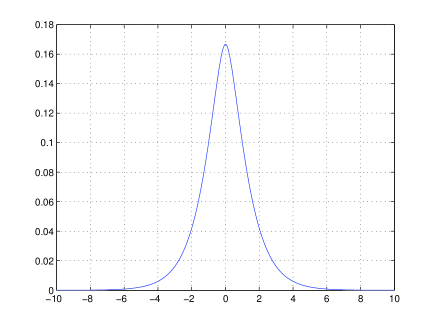
(a) $\rho(x)=\frac{1}{3}e^{-|x|}-\frac{1}{6}e^{-2|x|}$ profile.

(b) $\rho^{\prime}(x)=\left(\frac{1}{3}e^{-|x|}-\frac{1}{3}e^{-2|x|}\right)_{x<0}+\left(\frac{1}{3}e^{-2|x|}-\frac{1}{3}e^{-|x|}\right)_{x>0}$ profile.

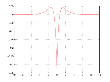
(c) $\rho^{\prime\prime}(x)=\frac{1}{3}e^{-|x|}-\frac{2}{3}e^{-2|x|}$ profile

Figure 1: Variation of the smooth-peakon with the amplitude $1/6$ at initial time.

Lemma 3.3 (Quadratic Identity; See [7]).

For any $u\in L^{2}(\mathbb{R})$ and $\xi\in\mathbb{R}$, it holds

$$E(u)-E(\varphi_{c})=\|u-\varphi_{c}(\cdot-\xi)\|^{2}_{\mathcal{H}}+4c\left(v(\xi)-\frac{c}{6}\right),$$ (3.10)

where $v=(4-\partial^{2}_{x})^{-1}u$ and $\rho_{c}(0)=c/6$.

Proof. We follow the idea of Constantin and Strauss with the CH equation (see [2], Lemma $1$). We compute

$$E(u-\varphi_{c}(\cdot-\xi)) =E(u)+E(\varphi_{c})-2\left\langle(1-\partial^{2}_{x})\varphi_{c}(\cdot-\xi),(4-\partial^{2}_{x})^{-1}u\right\rangle_{H^{-1},H^{1}}$$

$$=E(u)+E(\varphi_{c})-2\left\langle(1-\partial^{2}_{x})\varphi_{c}(\cdot-\xi),v\right\rangle_{H^{-1},H^{1}},$$ (3.11)

where $\langle\cdot,\cdot\rangle_{H^{-1},H^{1}}$ denotes the duality bracket $H^{-1}(\mathbb{R})$, $H^{1}(\mathbb{R})$. Now, using the definition of $\varphi^{\prime}_{c}(\cdot-\xi)$ and integration by parts, we have

$$\left\langle(1-\partial^{2}_{x})\varphi_{c}(\cdot-\xi),v\right\rangle_{H^{-1},H^{1}} =\int_{\mathbb{R}}v\varphi_{c}(\cdot-\xi)+\int_{\mathbb{R}}v_{x}\varphi^{\prime}_{c}(\cdot-\xi)$$

$$=\int_{\mathbb{R}}v\varphi_{c}(\cdot-\xi)+\int_{-\infty}^{\xi}v_{x}\varphi_{c}(\cdot-\xi)-\int_{\xi}^{+\infty}v_{x}\varphi_{c}(\cdot-\xi)$$

$$=2cv(\xi).$$ (3.12)

Recalling that the energy of peakons is given by

$$E(\varphi_{c}) =\left\langle(1-\partial^{2}_{x})\varphi_{c},(4-\partial^{2}_{x})^{-1}\varphi_{c}\right\rangle_{H^{-1},H^{1}}=\int_{\mathbb{R}}\rho_{c}\varphi_{c}+\int_{\mathbb{R}}\rho^{\prime}_{c}\varphi^{\prime}_{c}$$

$$=\int_{\mathbb{R}}\rho_{c}\varphi_{c}+\int_{-\infty}^{0}\rho^{\prime}_{c}\varphi_{c}-\int_{0}^{+\infty}\rho^{\prime}_{c}\varphi_{c}=2c\rho_{c}(0)=\frac{c^{2}}{3}\;,$$ (3.13)

we obtain the lemma. $\square$

Now we will study carefully the local extrema of $v=(4-\partial^{2}_{x})^{-1}u$. Let $u\in L^{2}(\mathbb{R})$ with $y=(1-\partial^{2}_{x})u\in\mathcal{M}^{+}(\mathbb{R})$, and assume that (3.6) holds for some $z\in\mathbb{R}$. We consider the interval in which the mass of smooth-peakons is concentrated, and the interval in which the mass of second derivative of smooth-peakons is strictly negative. In the sequel of this paper, the notation $\alpha\simeq\beta$ means that $0.9\times\beta\leq\alpha\leq 1.1\times\beta$. We set, for any $z\in\mathbb{R}$,

$$\Theta_{z}=[z-6.7,z+6.7],~{}~{}\text{where}~{}~{}6.7\simeq\text{ln}\left(\frac{20}{20-\sqrt{399}}\right),$$ (3.14)

and

$$\mathcal{V}_{z}=\left[z-\text{ln}\sqrt{2},z+\text{ln}\sqrt{2}\right].$$ (3.15)

One can clearly see that $\mathcal{V}_{0}$ is a subset of $\Theta_{0}$ (since $20/(20-\sqrt{399})>\sqrt{2}$). We chose the values $\pm 6.7$ such that $\rho_{c}(\pm 6.7)\simeq c/2400\simeq 4.1\times 10^{-4}c$ as in [6]. Also, we have $\rho^{\prime}_{c}(-6.7)=-\rho^{\prime}_{c}(6.7)\simeq 4.1\times 10^{-4}c$ and $\rho^{\prime\prime}_{c}(\pm 6.7)\simeq 4.1\times 10^{-4}c$. Then $\rho_{c}$, $\rho^{\prime}_{c}$ and $\rho^{\prime\prime}_{c}$ are very small with respect to the amplitude $c$ on $\mathbb{R}\setminus\Theta_{0}$.

We claim the following result.

Lemma 3.4 (Uniqueness of the Local Maximum).

Let $u\in L^{2}(\mathbb{R})$ with $y=(1-\partial^{2}_{x})u\in\mathcal{M}^{+}(\mathbb{R})$, that satisfies (3.6) for some $z\in\mathbb{R}$. There exists $\varepsilon_{0}>0$ only depending on the speed $c$, such that if $0<\varepsilon<\varepsilon_{0}$, then the function $v=(4-\partial^{2}_{x})^{-1}u$ admits a unique local extremum on $\Theta_{z}$. This extremum is a maximum, and it holds

$$v(x)\leq\frac{c}{300},~{}~{}\forall x\in\mathbb{R}\setminus\Theta_{z},$$ (3.16)

$$u(x)\leq\frac{c}{300},~{}~{}\forall x\in\mathbb{R}\setminus\Theta_{z}.$$ (3.17)

Proof. The key is to study the impact of the assumption $y\in\mathcal{M}^{+}(\mathbb{R})$ on $v$. First, let us show that $|v_{x}|\leq 2v$ on $\mathbb{R}$. We recall that from the assumption $y\geq 0$, we have $u\geq 0$ and $v\geq 0$ on $\mathbb{R}$. According to the definition of $v$, we have for all $x\in\mathbb{R}$,

$$v(x)=\frac{e^{-2x}}{4}\int_{-\infty}^{x}e^{2x^{\prime}}u(x^{\prime})dx^{\prime}+\frac{e^{2x}}{4}\int_{x}^{+\infty}e^{-2x^{\prime}}u(x^{\prime})dx^{\prime}$$

and

$$v_{x}(x)=-\frac{e^{-2x}}{2}\int_{-\infty}^{x}e^{2x^{\prime}}u(x^{\prime})dx^{\prime}+\frac{e^{2x}}{2}\int_{x}^{+\infty}e^{-2x^{\prime}}u(x^{\prime})dx^{\prime},$$

which yields

$$|v_{x}(x)|\leq 2v(x),~{}~{}\forall x\in\mathbb{R}.$$ (3.18)

Second, let us show that $u\leq 6v$ on $\mathbb{R}$. Using the Fourier transform, one can check that

$$(1-\partial^{2}_{x})^{-1}(4-\partial^{2}_{x})^{-1}(\cdot) =\mathcal{F}^{-1}\left[\frac{1}{3(1+\omega^{2})}-\frac{1}{3(4+\omega^{2})}\right](\cdot)$$

$$=\frac{1}{3}(1-\partial^{2}_{x})^{-1}(\cdot)-\frac{1}{3}(4-\partial^{2}_{x})^{-1}(\cdot),$$ (3.19)

and one can rewrite $v$ as

$$v=(4-\partial^{2}_{x})^{-1}(1-\partial^{2}_{x})^{-1}y=\frac{1}{3}(1-\partial^{2}_{x})^{-1}y-\frac{1}{3}(4-\partial^{2}_{x})^{-1}y.$$ (3.20)

Then for all $x\in\mathbb{R}$,

$$u(x)-6v(x) =-(1-\partial^{2}_{x})^{-1}y(x)+2(4-\partial^{2}_{x})^{-1}y(x)$$

$$=-\frac{1}{2}\int_{\mathbb{R}}e^{-|x-x^{\prime}|}y(x^{\prime})dx^{\prime}+\frac{1}{2}\int_{\mathbb{R}}e^{-2|x-x^{\prime}|}y(x^{\prime})dx^{\prime}$$

$$\leq 0,$$ (3.21)

since $e^{-2|\cdot|}\leq e^{-|\cdot|}$ on $\mathbb{R}$.

We are now ready to prove the uniqueness of local maxima in $\Theta_{z}$. Let us first study the sign of $v_{xx}$ on $\mathcal{V}_{z}$. One can easy check that for all $x\in\mathcal{V}_{0}$,

$$\rho^{\prime\prime}_{c}(x)\leq\frac{\sqrt{2}-2}{6}c.$$ (3.22)

Then, combining (3.8) and (3.22), taking $0<\varepsilon<\varepsilon_{0}$ with $\varepsilon_{0}\ll 1$, we have for all $x\in\mathcal{V}_{z}$,

$$v_{xx}(x)\leq\frac{\sqrt{2}-2}{6}c+O(\varepsilon^{1/4})\leq\frac{\sqrt{2}-2}{600}c<0,$$

which implies that $v_{x}$ is strictly decreasing on $\mathcal{V}_{z}$. Let us study the sign of $v_{x}$ on $\Theta_{z}\setminus\mathcal{V}_{z}$. One can easily check that

$$\rho^{\prime}_{c}\left(-\text{ln}\sqrt{2}\right)=\frac{\sqrt{2}-1}{6}c~{}~{}\text{and}~{}~{}\rho^{\prime}_{c}\left(\text{ln}\sqrt{2}\right)=-\frac{\sqrt{2}-1}{6}c,$$ (3.23)

and that $\rho^{\prime}_{c}(x)\geq 10^{-4}c$ for all $x\in[-6.7,-\text{ln}\sqrt{2}]$. Then using (3.9) and taking $0<\varepsilon<\varepsilon_{0}$ with $\varepsilon_{0}\ll 1$, we have $v_{x}(x)\geq 4\times 10^{-5}c>0$ for all $x\in[z-6.7,z-\text{ln}\sqrt{2}]$. Proceeding in the same way, we obtain $v_{x}(x)\leq-4\times 10^{-5}c<0$ for all $x\in[z+\text{ln}\sqrt{2},z+6.7]$. Since $v_{x}$ is strictly decreasing on $\mathcal{V}_{z}$ and changes sign, $v_{x}$ vanishes once on $\mathcal{V}_{z}$ and thus on $\Theta_{z}$. Hence, $v$ admits a single local extremum on $\Theta_{z}$, which is a maximum since $v_{xx}<0$ on $\mathcal{V}_{z}$.

Now, using that $\rho_{c}$ is increasing on $\mathbb{R}^{-}$, (3.9) and taking $0<\varepsilon<\varepsilon_{0}$ with $\varepsilon_{0}\ll 1$, it holds for all $x\in]-\infty,z-6.7[$,

$$v(x)=\rho_{c}(x-z)+O(\varepsilon^{1/4})\leq\frac{c}{2400}+O(\varepsilon^{1/4})\leq\frac{c}{300}.$$

Proceeding in the same way for $x\in]z+6.7,+\infty[$, we obtain (3.16).

Combining (3.8), (3) and proceeding as for the estimate (3.16), we get (3.17). Note that $\varphi_{c}(\pm 6.7)\simeq 1.2\times 10^{-3}c$. This completes the proof of the lemma. $\square$

Under the assumptions of Lemma 3.4, $v$ has got a unique point of global maximum on $\mathbb{R}$. In the sequel of this section, we will denote by $\xi$ this point of global maximum and we set $M=v(\xi)=\max_{x\in\mathbb{R}}v(x)$. The next two lemmas can be directly deduced from the similar lemmas established in [7] (see also [6]).

Lemma 3.5 (Connection Between $E(\cdot)$ and $M^{2}$; See [7]).

Let $u\in L^{2}(\mathbb{R})$ and $v=(4-\partial^{2}_{x})^{-1}u\in H^{2}(\mathbb{R})$. Define the function $g$ by

$$g(x)=\left\{\begin{aligned} &2v+v_{xx}-3v_{x},~{}~{}x<\xi,\\ &2v+v_{xx}+3v_{x},~{}~{}x>\xi.\\ \end{aligned}\right.$$ (3.24)

Then it holds

$$\int_{\mathbb{R}}g^{2}(x)dx=E(u)-12M^{2}.$$ (3.25)

Lemma 3.6 (Connection Between $F(\cdot)$ and $M^{3}$; See [7]).

Let $u\in L^{2}(\mathbb{R})$ and $v=(4-\partial^{2}_{x})^{-1}u\in H^{2}(\mathbb{R})$. Define the function $h$ by

$$h(x)=\left\{\begin{aligned} &-v_{xx}-6v_{x}+16v,~{}~{}x<\xi,\\ &-v_{xx}+6v_{x}+16v,~{}~{}x>\xi.\\ \end{aligned}\right.$$ (3.26)

Then it holds

$$\int_{\mathbb{R}}h(x)g^{2}(x)dx=F(u)-144M^{3}.$$ (3.27)

Sketch of proof. The proof of Lemmas 3.5-3.6 follows by direct computation, using integration by parts, with $v_{x}(\xi)=0$ and $v(\pm\infty)=v_{x}(\pm\infty)=v_{xx}(\pm\infty)=0$. See [7] (also [6]) to undersand the technique. $\square$

We can now connect the conservation laws.

Lemma 3.7 (Connection Between $E(\cdot)$ and $F(\cdot)$).

Let $u\in L^{2}(\mathbb{R})$, with $y=(1-\partial^{2}_{x})u\in{\mathcal{M}}^{+}({\mathbb{R}})$, that satisfies (3.6) for some $z\in\mathbb{R}$. There exists $\varepsilon_{0}>0$ only depending on the speed $c$, such that if $0<\varepsilon<\varepsilon_{0}$, then it holds

$$M^{3}-\frac{1}{4}E(u)M+\frac{1}{72}F(u)\leq 0.$$ (3.28)

Proof. The key is to show that $h\leq 18M$ on $\mathbb{R}$. Note that by (3.9) we know that $18M\geq c/4$ and that Lemma 3.4 ensures that $\xi\in\Theta_{z}$ for $\varepsilon_{0}$ small enough. Let us set $\lambda=z-6.7$, $\mu=z+6.7$, and rewrite the function $h$ as

$$h(x)=\left\{\begin{aligned} &-v_{xx}-6v_{x}+16v,~{}~{}x<\lambda,\\ &u-6v_{x}+12v,~{}~{}\lambda<x<\xi,\\ &u+6v_{x}+12v,~{}~{}\xi<x<\mu,\\ &-v_{xx}+6v_{x}+16v,~{}~{}x>\mu\;.\\ \end{aligned}\right.$$

If $x\in\mathbb{R}\setminus\Theta_{z}$, using that $v_{xx}=4v-u$, (3.16) and (3.17), it holds

$$h \leq|v_{xx}|+6|v_{x}|+16v\leq u+32v\leq\frac{c}{9}\leq 18M.$$

If $\lambda<x<\xi$, then $v_{x}\geq 0$, and using that $u\leq 6v$ on $\mathbb{R}$, we have

$$h=u-6v_{x}+12v\leq 18v.$$

If $\xi<x<\mu$, then $v_{x}\leq 0$, and similarly using that $u\leq 6v$ on $\mathbb{R}$, we get

$$h=u+6v_{x}+12v\leq 18v.$$

Therefore, it holds

$$h(x)\leq 18\max_{x\in\mathbb{R}}v(x)=18M,~{}~{}\forall x\in\mathbb{R}.$$ (3.29)

Now, combining (3.25), (3.27) and (3.29), we get

$$F(u)-144M^{3}=\int_{\mathbb{R}}h(x)g^{2}(x)dx\leq\|h\|_{L^{\infty}(\mathbb{R})}\int_{\mathbb{R}}g^{2}(x)dx\leq 18M(E(u)-12M^{2}),$$

and we obtain the lemma. $\square$

Proof of Theorem 3.1. We argue as El Dika and Molinet in [4]. As noticed after the statement of the theorem, it suffices to prove (3.7) assuming that $u\in L^{2}(\mathbb{R})$ satisfies (3.1), (3.2) and (3.6). We recall that $M=v(\xi)=\max_{x\in\mathbb{R}}v(x)$ and we set $\delta=c/6-M$. We first remark that if $\delta\leq 0$, combining (3.4) and (3.10), it holds

$$\|u-\varphi_{c}(\cdot-\xi)\|_{\mathcal{H}}\leq|E(u_{0})-E(\varphi_{c})|^{1/2}\leq O(\varepsilon),$$

that yields the desired result. Now suppose that $\delta>0$, that is the maximum of the function $v$ is less than the maximum of $\rho_{c}$. Combining (3.4), (3.5) and (3.28), we get

$$M^{3}-\frac{1}{4}E(\varphi_{c})M+\frac{1}{72}F(\varphi_{c})\leq O(\varepsilon^{2}).$$

Using that $E(\varphi_{c})=c^{2}/3$ and $F(\varphi_{c})=2c^{3}/3$, our inequality becomes

$$\left(M-\frac{c}{6}\right)^{2}\left(M+\frac{c}{3}\right)\leq O(\varepsilon^{2}).$$

Next, substituting $M$ by $c/6-\delta$ and using that $[M+c/3]^{-1}<3/c$, we obtain

$$\delta^{2}\leq O(\varepsilon^{2})\Rightarrow\delta\leq O(\varepsilon).$$ (3.30)

Finally, combining (3.4), (3.10) and (3.30), we infer that

$$\|u-\varphi_{c}(\cdot-\xi)\|_{\mathcal{H}}\leq C\sqrt{\varepsilon},$$

where $C>0$ only depends on the speed $c$. This completes the proof of the stability of peakons.

Acknowledgements.

The author would like to thank his PhD advisor Luc Molinet for his help and his careful reading of this manuscript.

References

[1]
Adrian Constantin and David Lannes.
The hydrodynamical relevance of the Camassa-Holm and
Degasperis-Procesi equations.
Arch. Ration. Mech. Anal., 192(1):165–186, 2009.
[2]
Adrian Constantin and Walter A. Strauss.
Stability of peakons.
Comm. Pure Appl. Math., 53(5):603–610, 2000.
[3]
A. Degasperis, D. D. Kholm, and A. N. I. Khon.
A new integrable equation with peakon solutions.
Teoret. Mat. Fiz., 133(2):170–183, 2002.
[4]
Khaled El Dika and Luc Molinet.
Stability of multipeakons.
Ann. Inst. H. Poincaré Anal. Non Linéaire,
26(4):1517–1532, 2009.
[5]
Joachim Escher, Yue Liu, and Zhaoyang Yin.
Global weak solutions and blow-up structure for the
Degasperis-Procesi equation.
J. Funct. Anal., 241(2):457–485, 2006.
[6]
André Kabakouala.
Stability in the energy space of the sum of peakons for the
Degasperis–Procesi equation.
J. Differential Equations, 259(5):1841–1897, 2015.
[7]
Zhiwu Lin and Yue Liu.
Stability of peakons for the Degasperis-Procesi equation.
Comm. Pure Appl. Math., 62(1):125–146, 2009.
[8]
Yue Liu and Zhaoyang Yin.
Global existence and blow-up phenomena for the Degasperis-Procesi
equation.
Comm. Math. Phys., 267(3):801–820, 2006.