Dipolar fermions in a multilayer geometry

Abstract

We investigate the behavior of identical dipolar fermions with aligned dipole moments in two-dimensional multilayers at zero temperature. We consider density instabilities that are driven by the attractive part of the dipolar interaction and, for the case of bilayers, we elucidate the properties of the stripe phase recently predicted to exist in this interaction regime. When the number of layers is increased, we find that this “attractive” stripe phase exists for an increasingly larger range of dipole angles, and if the interlayer distance is sufficiently small, the stripe phase eventually spans the full range of angles, including the situation where the dipole moments are aligned perpendicular to the planes. In the limit of an infinite number of layers, we derive an analytic expression for the interlayer effects in the density-density response function and, using this result, we find that the stripe phase is replaced by a collapse of the dipolar system.

I Introduction

Motivated by the prospect of novel many-body phases generated by anisotropic long-range dipolar interactions, much attention has recently been devoted to ultracold polar molecules and magnetic atoms Baranov (2008); Lahaye et al. (2009); Baranov et al. (2012). Dipolar fermions, in particular, can be used to simulate strongly correlated phenomena in electron systems, including charge density modulations (stripes) and unconventional superconductivity Grüner (1988); Kivelson et al. (1998, 2003).

Quantum degeneracy has already been achieved for dipolar Fermi gases of atoms with a permanent magnetic dipole moment such as chromium Naylor et al. (2015), dysprosium Lu et al. (2012) and erbium Aikawa et al. (2014a). This has enabled the observation of dipole-driven Fermi surface deformations in the Fermi liquid phase Aikawa et al. (2014b). However, to investigate many-body phenomena at stronger dipole-dipole interactions, it appears necessary to use polar molecules, which generally possess larger dipole moments — the electric dipole moment can be as large as 5.5 Debye in the case of ¹³³Cs⁶Li Carr et al. (2009). Thus far, there has been major progress towards producing quantum degenerate clouds of long-lived fermionic dipolar molecules using ⁴⁰K⁸⁷Rb Ni et al. (2008); Ospelkaus et al. (2010); Ni et al. (2010), ²³Na⁶Li Heo et al. (2012), ¹³³Cs⁶Li Repp et al. (2013), and ²³Na⁴⁰K Wu et al. (2012); Park et al. (2015).

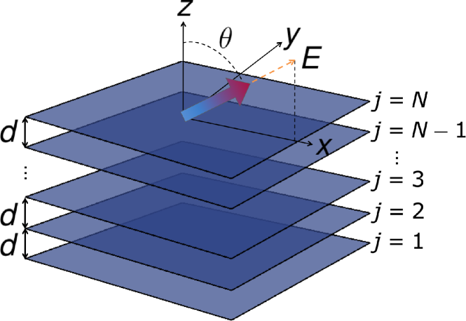
Figure 1: (Color online) Schematic representation of the system geometry. A gas of dipolar fermions is confined to $N$ 2D layers labelled by an index $j=1,2,\dots,N$ and separated by a distance $d$. We assume that each layer has the same density of dipoles $n$. The dipole moment of each fermion is aligned by an electric field ${\mathbf{E}}=(E_{x},0,E_{z})$ in the $x$-$z$ plane ($\varphi=0$ direction), at an angle $\theta$ with respect to the $\hat{{\mathbf{z}}}$ direction.

The dipole-dipole interaction can be further tuned and enhanced by confining the polar molecules to two-dimensional (2D) layers. Such a geometry has been used to suppress chemical reactions de Miranda et al. (2011) and to stabilize the gas against mechanical collapse, which arises in three dimensions for a sufficiently strong interaction Miyakawa et al. (2008); Sogo et al. (2009); Endo et al. (2010); Zhang and Yi (2009, 2010); Krieg et al. (2015); Baillie et al. (2015). Furthermore, by aligning all the dipole moments with a strong electric field, the nature of the effective 2D dipolar interaction within the plane may be externally manipulated: The dipole-dipole repulsion is maximized by aligning the dipole moments perpendicular to the plane, while anisotropy and attraction are gradually introduced by varying the dipole tilt (see Fig. 1). This possibility has stimulated much theoretical work on dipolar fermionic gases in single and multilayer 2D geometries Baranov et al. (2012).

For the single-layer geometry and for small (but non-zero) tilting angles, the weakly interacting system corresponds to a Landau Fermi liquid with deformed Fermi surface Lu and Shlyapnikov (2012), similarly to the case in 3D. With increasing dipolar interaction (or cloud density), the system is then predicted to undergo a transition to a uni-directional density modulated phase Yamaguchi et al. (2010); Sun et al. (2010); Babadi and Demler (2011); Sieberer and Baranov (2011), where the modulations are perpendicular to the direction of the dipole tilt. Such a “stripe” phase has also been shown to exist in the isotropic case where the dipoles are aligned perpendicular to the layer, thus requiring the system to spontaneously break the rotational symmetry Parish and Marchetti (2012). This result has recently been supported by density functional theory calculations van Zyl et al. (2015), which predict a transition to a stripe phase followed by a transition to a triangular Wigner crystal at higher coupling. Quantum Monte Carlo calculations also find a Wigner crystal phase for the case of perpendicularly aligned dipoles, although at a much higher dipolar interaction than that obtained from density functional theory Matveeva and Giorgini (2012).

For tilting angles greater than a critical angle, the attractive part of the dipolar interaction can lead to $p$-wave superfluidity in the single-layer system Bruun and Taylor (2008), and this phase may even coexist with stripe order Wu et al. (2015). A sufficiently strong attraction eventually drives a mechanical instability of the cloud towards collapse Bruun and Taylor (2008); Yamaguchi et al. (2010); Sieberer and Baranov (2011); Parish and Marchetti (2012); Block and Bruun (2014). However, interestingly, if one instead considers a bilayer geometry, the additional layer stabilizes the collapse at large tilt angles — as long as the dipoles are aligned out of the plane ($\theta<\pi/2$) — to form a new stripe phase, where the density modulations are oriented along the direction of the dipole tilt Marchetti and Parish (2013).

In this article, we investigate such a stripe phase, which is generated by the attractive part of the dipolar interaction for large enough dipole tilt angle. We start by elucidating its properties in the case of the bilayer, where we provide a classical argument for how the stripes in each layer are shifted with respect to each other. Then we extend our results for the density-density response function to the multilayer geometry. We employ an approach based on the STLS scheme Singwi et al. (1968); Parish and Marchetti (2012); Marchetti and Parish (2013) that incorporates exchange interactions only, which should be reasonable for the “attractive” stripe phase Marchetti and Parish (2013), although note that we neglect the possibility of pairing Pikovski et al. (2010); Matveeva and Giorgini (2014) and other stripe phases driven by the strong repulsion Block et al. (2012); Marchetti and Parish (2013). As the number of layers $N$ is increased, we find that the attractive stripe phase spans an increasingly larger region of the phase diagram. However, this stripe phase eventually gives way to collapse in the $N\to\infty$ limit.

The paper is organized as follows: In Sec. II, we describe the system geometry and introduce the STLS scheme which allows us to evaluate the density-density response function matrix in the multilayer geometry; in Sec. III, we describe the properties of the density instabilities driven by the attractive part of the interlayer dipolar interaction and, in Sec. III.1, we explain via a classical model how the stripes in each layer are shifted with respect to each other. In Sec. IV we extend the results to a generic number of layers $N$, while, in Sec. V we consider the $N\to\infty$ limit. The concluding remarks are gathered in Sec. VI.

II Multilayer system and model

We consider a gas of polar fermionic molecules in a multilayer geometry, as shown in the schematic picture in Fig. 1. The molecules have a dipole moment $D$ and are confined to $N$ two-dimensional layers, each labelled by an index $j=1,2,\dots,N$, and equally separated by a distance $d$. We assume that the dipoles are aligned by an external electric field ${\mathbf{E}}=(E_{x},0,E_{z})$ in the $x$-$z$ plane, which is tilted at an angle $\theta$ with respect to the $\hat{{\mathbf{z}}}$ direction. Within each layer, we parameterize the $x$-$y$ in-plane wavevector by polar coordinates ${\mathbf{q}}=(q,\varphi)$, where $\varphi=0$ corresponds to the direction of the dipole tilt.

In the limit $qW\ll 1$, where $W$ is the layer width, the effective 2D intralayer interaction between dipoles takes the following form Fischer (2006):

$$v_{jj}({\mathbf{q}})\equiv v({\mathbf{q}})=V_{0}-2\pi D^{2}q\xi(\theta,\varphi)\;,$$ (1)

where $\xi(\theta,\varphi)=\cos^{2}\theta-\sin^{2}\theta\cos^{2}\varphi$. Here, ${\mathbf{q}}$ corresponds to the relative wavevector between two dipoles. The constant $V_{0}$ is a short-range contact interaction term that in general depends on the width $W$ Fischer (2006), yielding a natural UV cut-off. Since we are considering identical fermions, the system properties will not depend on $V_{0}$.

In the limit where the layer width is much smaller than the layer separation, $W\ll d$, the interaction between two dipoles in different layers $j>l$ is given by Li et al. (2010):

$$v_{jl}({\mathbf{q}})=-2\pi D^{2}qe^{-(j-l)qd}\left[\xi(\theta,\varphi)+i\sin 2\theta\cos\varphi\right]\;.$$ (2)

The remaining interlayer interactions can be obtained from the condition $v_{lj}({\mathbf{q}})=v_{jl}(-{\mathbf{q}})=v^{*}_{jl}({\mathbf{q}})$, which is derived from the fact the the dipolar interaction is always real in real space. Likewise, the momentum-space interaction is complex for $\theta\neq 0$ since the real-space interaction is not invariant under the transformation ${\mathbf{r}}\mapsto-{\mathbf{r}}$.

Assuming that each layer has the same density $n$, we define the Fermi wavevector $k_{F}=\sqrt{4\pi n}$. This allows us to define the dimensionless interaction strength $U=mD^{2}k_{F}/\hbar^{2}$, where $m$ is the fermion mass. The other parameters that can be independently varied are the dipole tilt angle $\theta$ and the dimensionless layer separation $k_{F}d$.

II.1 Response function and STLS equations

Similarly to Ref. Marchetti and Parish (2013), we make use of linear response theory to analyze density wave instabilities. In the multilayer system, the linear density response $\delta n$ to an external perturbing potential $V^{ext}$ defines the density-density response function matrix Zheng and MacDonald (1994),

$$\delta n_{j}({\mathbf{q}},\omega)=\sum_{l}\chi_{jl}({\mathbf{q}},\omega)V_{l}^{ext}({\mathbf{q}},\omega)\;,$$ (3)

where $j,l$ are the layer indices. A divergence in the static density-density response function matrix $\chi_{jl}({\mathbf{q}},\omega=0)$ signals an instability of the system. Specifically, the system is unstable towards forming a stripe phase when the smallest eigenvalue $\tilde{\chi}_{\text{min}}({\mathbf{q}})$ of the static response function matrix first diverges at a critical value of the wavevector ${\mathbf{q}}_{c}=(q_{c},\varphi_{c})$.

While the response function is known exactly for the non-interacting gas, typically one can only incorporate the effect of interactions approximately. A standard approach is the random phase approximation (RPA), where one replaces the external potential with one that contains an effective potential due to the perturbed density: $V_{j}^{ext}\mapsto V_{j}^{ext}+\sum_{l}v_{jl}\delta n_{l}$. However, RPA neglects exchange correlations, which are always important in the dipolar system, even in the long-wavelength limit $q\to 0$ Parish and Marchetti (2012). This issue may be remedied using a conserving Hartree-Fock approximation Babadi and Demler (2011); Sieberer and Baranov (2011); Block et al. (2012), but we choose a simpler and physically motivated approach where correlations are included via local field factors $G_{jl}({\mathbf{q}})$ Giuliani and Vignale (2005). This yields the inverse density-density response function matrix

$$\hat{\chi}^{-1}{}_{jl}({\mathbf{q}},\omega)=\displaystyle\frac{\delta_{jl}}{\Pi({\mathbf{q}},\omega)}-v_{jl}({\mathbf{q}})\left[1-G_{jl}({\mathbf{q}})\right]\;,$$ (4)

where $\Pi({\mathbf{q}},\omega)$ is the non-interacting response function, which, for equal density layers, reads as Stern (1967); Zheng and MacDonald (1994)

$$\Pi({\mathbf{q}},i\omega)=\frac{m}{2\pi\hbar^{2}b}\left\{\sqrt{2}\left[a+\sqrt{a^{2}+\left(\omega b\right)^{2}}\right]^{1/2}-b\right\}\;,$$

with $a=\frac{b^{2}}{4}-b\frac{k_{F}^{2}}{m}-\omega^{2}$ and $b=\frac{q^{2}}{m}$. RPA corresponds to taking the limit where the layer-resolved local field factors $G_{jl}({\mathbf{q}})$ in Eq. (4) are all zero.

The response function (4) can be related to the layer-resolved static structure factor $S_{jl}({\mathbf{q}})$ by the fluctuation-dissipation theorem:

$$S_{jl}({\mathbf{q}})=-\frac{\hbar}{\pi n}\int_{0}^{\infty}d\omega\chi_{jl}({\mathbf{q}},i\omega)\;.$$ (5)

In the non-interacting limit, the static structure factor is diagonal, i.e., $S_{jl}^{(0)}({\mathbf{q}})=\delta_{jl}\ S^{(0)}(q)$, and can be evaluated exactly (see App. A), where

$$S^{(0)}(q)=\frac{2}{\pi}\arcsin\left(\displaystyle\frac{q}{2k_{F}}\right)+\frac{q}{\pi k_{F}}\sqrt{1-\left(\frac{q}{2k_{F}}\right)^{2}}\;,$$ (6)

for $q\leq 2k_{F}$, while $S^{(0)}(q)=1$ for $q>2k_{F}$ Zheng and MacDonald (1994); Giuliani and Vignale (2005).

To determine the local field factors, we consider the STLS approximation scheme, where we have the expression Singwi et al. (1968); Zheng and MacDonald (1994):

$$G_{jl}({\mathbf{q}})=\frac{1}{n}\int\frac{d{\mathbf{k}}}{(2\pi)^{2}}\frac{{\mathbf{q}}\cdot{\mathbf{k}}}{q^{2}}\frac{v_{jl}({\mathbf{k}})}{v_{jj}({\mathbf{q}})}\left[\delta_{jl}-S_{jl}({\mathbf{q}}-{\mathbf{k}})\right]\;.$$ (7)

In principle, $G_{jl}({\mathbf{q}})$ can be determined self-consistently by solving Eqs. (4), (5) and (7). Note that this self-consistent approach includes all correlations beyond RPA and is not just limited to exchange correlations. As such, the STLS scheme has proven to be a powerful method for treating strongly correlated electron systems such as the 2D electron gas Giuliani and Vignale (2005). We previously adapted an improved version of this scheme to the dipolar system, both in the single- Parish and Marchetti (2012) and double-layer Marchetti and Parish (2013) geometries. The scheme is improved by imposing, at each iteration step, the condition that the intralayer pair correlation function is zero at zero distance, $g_{jj}(0)=0$, where,

$$g_{jl}({\mathbf{r}})=1+\frac{1}{n}\int\frac{d{\mathbf{q}}}{(2\pi)^{2}}e^{i{\mathbf{q}}\cdot{\mathbf{r}}}\left[S_{jl}({\mathbf{q}})-\delta_{jl}\right]\;.$$ (8)

This ensures that the intralayer static structure factor $S_{jj}({\mathbf{q}})$ is dominated by Pauli exclusion in the long wavelength limit, $q\gg 2k_{F}$, and that the system response is independent of the short-range contact interaction term $V_{0}$ and the cut-off $W$.

In the following, we first review the bilayer case and describe the instability to a stripe phase occurring for large tilt angles $\theta$, where the modulations are oriented along the dipole tilt, i.e., along $\varphi=0$. We then show how the instability to the $\varphi=0$ stripe phase can be well described using exchange correlations only, and we use this to investigate its existence in the multilayer geometry.

III The $\varphi=0$ stripe phase in bilayers

The case of two layers ($N=2$) was previously analysed within the STLS self-consistent approximation scheme in Ref. Marchetti and Parish (2013). Here, at sufficiently small tilt angles $\theta<\theta_{c}$, and by increasing the value of the dimensionless coupling strength $U$, there is an instability from the uniform phase to a stripe phase with modulations along the $y$-axis ($\varphi=\pi/2$ stripe phase). The instability to this stripe phase is driven by intralayer correlations beyond exchange, which are induced by the repulsive part of the intralayer interaction potential $v({\mathbf{q}})$. By contrast, for $\theta_{c}<\theta<\pi/2$, the system develops an instability to a stripe phase along the $x$-axis ($\varphi=0$ stripe phase). While for a single layer, the attractive sliver of the intralayer interaction produces a collapse of the dipolar Fermi gas at large tilt angles, the bilayer geometry stabilizes the collapse in favour of a $\varphi=0$ stripe phase, which thus derives from a competition between the intralayer attraction in the $\varphi=0$ direction and the interlayer interaction.

Interestingly, this latter stripe phase can be accurately described using intralayer exchange correlations only. In fact, it was found for this phase that the intralayer pair correlation function $g_{jj}({\mathbf{r}})$ deviated only slightly from the non-interacting case, while the interlayer correlation function $g_{12}({\mathbf{r}})\sim 1$. In terms of local correlations, the interlayer local field factor can thus be neglected, $G_{12}({\mathbf{r}})=0$, while the intralayer one $G_{jj}({\mathbf{q}})\equiv G({\mathbf{q}})$ is determined from the non-interacting intralayer structure factor (6):

$$G({\mathbf{q}})=\frac{1}{n}\int\frac{d{\mathbf{k}}}{(2\pi)^{2}}\frac{{\mathbf{q}}\cdot{\mathbf{k}}}{q^{2}}\frac{v({\mathbf{k}})}{v({\mathbf{q}})}\left[1-S^{(0)}(q)\right]\;.$$ (9)

We refer to this approximation scheme as the exchange-only STLS approximation (X-STLS). For the single-layer case Parish and Marchetti (2012), this approach yielded an instability towards collapse at large $\theta$ that agreed with the predictions from Hartree-Fock calculations Bruun and Taylor (2008); Yamaguchi et al. (2010); Babadi and Demler (2011); Sieberer and Baranov (2011).

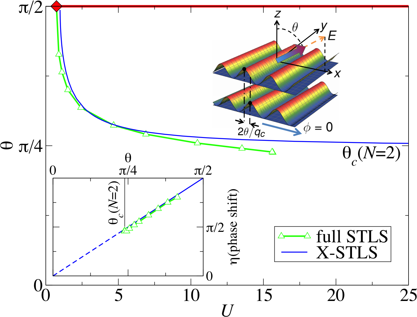
Figure 2: (Color online) Main panel: Phase boundary for the $\varphi=0$ stripe phase in the two-layer geometry as a function of the tilt angle $\theta$ and the dimensionless interaction strength $U$ at fixed interlayer distance $k_{F}d=2$. Density modulations are in the direction $\varphi=0$ of the dipole tilt (schematic figure). The instability to this phase is to the right of the plotted boundaries: The full STLS results Marchetti and Parish (2013) ([green] open triangles) are compared to the results obtained with exchange-only correlations ([blue] solid line), also referred to as the X-STLS approximation scheme. Within X-STLS, the $\varphi=0$ stripe phase appears for $\theta>\theta_{c}\simeq 0.79$. At $\theta=\pi/2$, the gas is unstable towards mechanical collapse for $U\gtrsim 1.57$ ([red] diamond symbol and thick solid line), where the gas compressibility is infinite. The density modulations in the two layers have a phase shift $\eta$ (lower inset) equal to $2\theta$, i.e., the shift between the modulations $2\theta/q_{c}$ (schematic figure).

The phase boundary between the normal phase and the $\varphi=0$ stripe phase obtained from the full STLS scheme is displayed in Fig. 2 ([green] open triangles) and is compared with the results of the X-STLS approximation ([blue] solid line). The value of the critical tilt angle for such a phase is $\theta_{c}\simeq 0.75$ if evaluated within the full STLS scheme, while it is slightly higher, $\theta_{c}\simeq 0.79$, if evaluated within the X-STLS approximation. It turns out that, for the phase boundary, the X-STLS approximation works particularly well at large angles, all the way up to $\theta=\pi/2$, where, for $U\gtrsim 1.57$ ([red] diamond symbol and thick solid line), the gas collapses because the Fermi pressure is not high enough to counteract the strong dipolar attraction.

The eigenvectors of the density-density response function (4) determine the phase-shift $\eta$ between layers, and for the bilayer geometry we have found that Marchetti and Parish (2013):

$$e^{i\eta}=-\displaystyle\frac{v_{12}({\mathbf{q}})[1-G_{12}({\mathbf{q}})]}{|v_{12}({\mathbf{q}})[1-G_{12}({\mathbf{q}})]|}\;.$$ (10)

For both $\varphi=\pi/2$ and $\varphi=0$ stripe phases, we find that the interlayer phase shift between the modulations is independent of the dipole interaction strength $U$ and the layer distance $d$. In particular, for the $\varphi=\pi/2$ stripe phase, both the interaction and the local field factor are real and thus both layer modulations are always in phase, i.e., $\eta=0$. On the other hand, for the $\varphi=0$ stripe phase, if we consider an exchange-only approximation (X-STLS) for which $G_{12}({\mathbf{q}})=0$, we obtain a phase shift of $\eta=2\theta$. The phase shift for the $\varphi=0$ stripe phase is plotted in the inset of Fig. 2. We see a very good agreement between the full STLS results ([green] open triangles) and the simplified X-STLS scheme ([blue] solid line). The $\varphi=0$ result may at first appear counter-intuitive, but it can be reproduced by evaluating the classical interaction energy between an infinite layer of dipoles in one layer and a single dipole in the second layer, as we discuss next.

III.1 Classical model

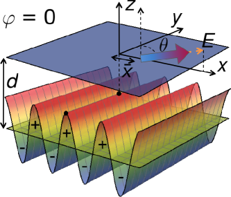
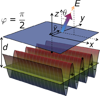
Figure 3: (Color online) Schematic representation of a single dipole in the top layer interacting classically with an infinite bottom layer of dipoles arranged in a stripe modulated phase. As in Fig. 1, all dipoles are aligned by an electric field $\mathbf{E}$. In the left (right) panel, the single dipole is shifted by $\bar{x}$ ($\bar{y}$) with respect to one of the stripe crests for the $\varphi=0$ ($\varphi=\frac{\pi}{2}$) stripe phase.

For the bilayer geometry, a simple classical model can easily explain the phase shifts found in both $\varphi=0$ and $\varphi=\pi/2$ stripe phases. Let us consider the simplified case of an infinite layer of dipoles whose density is modulated sinusoidally with a wavevector $q_{c}=2\pi/\lambda_{c}$ and amplitude $\rho_{0}$. We further assume that this interacts classically with a single dipole positioned at ${\mathbf{r}}_{0}$ in the other layer. The two layer densities are thus respectively given by:

$$\rho^{(1)}({\mathbf{r}}) =n+\rho_{0}\cos({\mathbf{q}}_{c}\cdot{\mathbf{r}})$$ (11)

$$\rho^{(2)}({\mathbf{r}}^{\prime}) =\delta({\mathbf{r}}^{\prime}-{\mathbf{r}}_{0})\;.$$ (12)

For the $\varphi=0$ ($\varphi=\pi/2$) stripe phase we have $\hat{{\mathbf{q}}}_{c}=\hat{{\mathbf{x}}}$ ($\hat{{\mathbf{q}}}_{c}=\hat{{\mathbf{y}}}$) and ${\mathbf{r}}_{0}=(\bar{x},0)$ (${\mathbf{r}}_{0}=(0,\bar{y})$) — see the schematic representation of both geometries in Fig. 3. The classical interaction energy is given by

$$E_{cl}=\int d{\mathbf{r}}d{\mathbf{r}}^{\prime}\rho^{(1)}({\mathbf{r}})v_{12}({\mathbf{r}}-{\mathbf{r}}^{\prime})\rho^{(2)}({\mathbf{r}}^{\prime})\;,$$ (13)

where

$$v_{12}({\mathbf{r}})=D^{2}\frac{x^{2}+y^{2}+d^{2}-3(x\sin\theta+d\cos\theta)^{2}}{(x^{2}+y^{2}+d^{2})^{5/2}}$$

is the interlayer potential (assuming that the distance $d$ is much larger than the layer thickness $W$). For a uniform density distribution $\rho^{(1)}({\mathbf{r}})=n$, the classical interaction energy would be zero; therefore only deviations from the average density in $\rho^{(1)}({\mathbf{r}})$ contribute (either positively or negatively) to $E_{cl}$.

Considering the Fourier transforms $\rho^{(1,2)}({\mathbf{r}})=\int\frac{d{\mathbf{q}}}{(2\pi)^{2}}\rho^{(1,2)}({\mathbf{q}})e^{i{\mathbf{q}}\cdot{\mathbf{r}}}$ and $v_{12}({\mathbf{r}})=\int\frac{d{\mathbf{q}}}{(2\pi)^{2}}v_{12}({\mathbf{q}})e^{i{\mathbf{q}}\cdot{\mathbf{r}}}$, we can rewrite (13) to obtain

$$E_{cl}=\int\displaystyle\frac{d{\mathbf{q}}}{(2\pi)^{2}}\rho^{(1)}(-{\mathbf{q}})v_{12}({\mathbf{q}})\rho^{(2)}({\mathbf{q}})\;,$$ (14)

where

$$\rho^{(1)}({\mathbf{q}}) =(2\pi)^{2}\left[n\delta({\mathbf{q}})+\rho_{0}\displaystyle\frac{\delta({\mathbf{q}}+{\mathbf{q}}_{c})+\delta({\mathbf{q}}-{\mathbf{q}}_{c})}{2}\right]$$

$$\rho^{(2)}({\mathbf{q}}) =e^{-i{\mathbf{q}}\cdot{\mathbf{r}}_{0}}\;.$$

Thus, as $v_{12}(0)=0$, we get in general

$$E_{cl}=\displaystyle\frac{\rho_{0}}{2}\left[v_{12}(-{\mathbf{q}}_{c})e^{i{\mathbf{q}}_{c}\cdot{\mathbf{r}}_{0}}+v_{12}({\mathbf{q}}_{c})e^{-i{\mathbf{q}}_{c}\cdot{\mathbf{r}}_{0}}\right]\;,$$ (15)

and specifically for the two stripe phases:

$$E_{cl}^{\varphi=0} =-\displaystyle\frac{4\pi^{2}D^{2}\rho_{0}}{\lambda_{c}}e^{-2\pi d/\lambda_{c}}\cos\left(2\pi\displaystyle\frac{\bar{x}}{\lambda_{c}}-2\theta\right)$$

$$E_{cl}^{\varphi=\pi/2} =-\displaystyle\frac{4\pi^{2}D^{2}\rho_{0}}{\lambda_{c}}e^{-2\pi d/\lambda_{c}}\cos^{2}\theta\cos\left(2\pi\displaystyle\frac{\bar{y}}{\lambda_{c}}\right)\;.$$

Therefore, we can conclude that, for both stripe configurations, the distance, $\bar{x}$ or $\bar{y}$, that minimizes the interaction energy $E_{cl}$ does not depend on the dipole strength $D$ or the layer separation $d$. Further, for the $\varphi=\pi/2$ stripe phase, the best configuration is the one where the single dipole in layer $2$ aligns with the maximum density of layer $1$, i.e., $\bar{y}_{\text{min}}=0$. By contrast, for the $\varphi=0$ stripe phase, the optimal configuration is for a phase shift equal to twice the dipole tilt angle $\theta$, i.e., $2\pi\bar{x}_{\text{min}}/\lambda_{c}=2\theta$. An analogous calculation was carried out for the $\varphi=\pi/2$ stripe phase in the simplified limit where the density modulations were approximated as discrete dipolar wires Block et al. (2012).

We now wish to extend these results to multiple layer $N>2$ configurations. We have seen that the presence of a second layer stabilises the region of collapse at large tilt angles $\theta_{c}<\theta<\pi/2$, replacing it with a novel stripe phase oriented along $\varphi=0$ Marchetti and Parish (2013). Furthermore, within the X-STLS approximation, the critical tilt angle for the $\varphi=0$ stripe phase in bilayers is $\theta_{c}(N=2)\sim 0.79$, which is lower than that for collapse in the single layer, $\theta_{c}(N=1)\sim 0.89$. It is therefore natural to ask whether the $\varphi=0$ stripe phase will tend to dominate the phase diagram as the number of layers $N$ is increased.

IV $N$ layers

Motivated by the results obtained for the bilayer system, we now apply the X-STLS approximation scheme to the general case of finite $N>2$ layers and evaluate the occurrence of the $\varphi=0$ stripe phase when varying the system parameters. In particular, by neglecting all correlations except for the exchange ones, we assume that all off-diagonal local field factors are zero, $G_{j\neq l}({\mathbf{q}})=0$, while the intralayer ones $G({\mathbf{q}})$ are evaluated according to Eq. (9). To locate the stripe instabilities, we extract the smallest eigenvalue of the static density-density response function matrix, $\tilde{\chi}_{\text{min}}({\mathbf{q}})$, and determine the critical wavevector ${\mathbf{q}}_{c}=(q_{c},\varphi_{c})$ at which it first diverges. If the instability is for a specific angle $\varphi_{c}$, then it signals the formation of a density wave with modulations in that direction and with a period set by $q_{c}$. Here, we always find that $\varphi_{c}=0$, as in the bilayer case.

At the stripe transition, the phase shifts $\eta_{jl}$ between the stripes in different layers $j,l$ are extracted from the eigenvector associated with the smallest eigenvalue, $\tilde{\chi}_{\text{min}}({\mathbf{q}}_{c})$. We find that the behavior of the multilayer system is a natural extension of the bilayer case: the phase shift between nearest neighbour layers $\eta_{jj+1}$ grows monotonically with the tilt angle $\theta$, although linearly only for small values of $\theta$. Moreover, the phase shift between more distant layers is always proportional to $\eta_{jj+1}$.

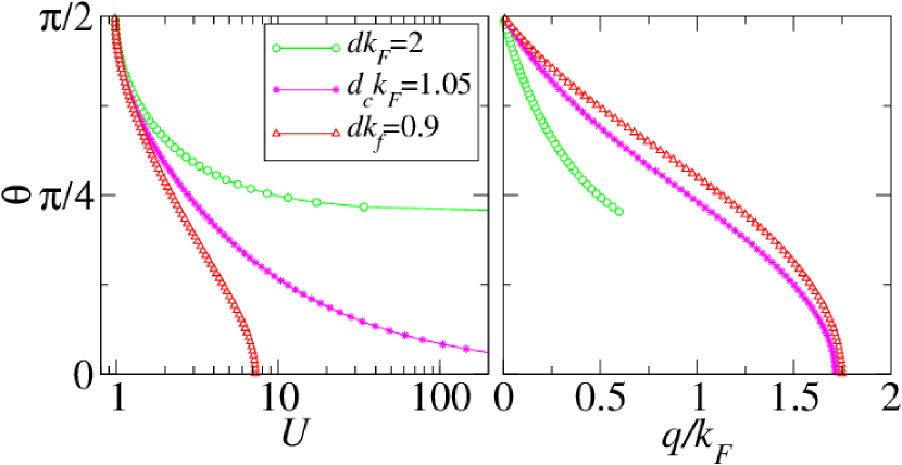
Figure 4: (Color online) Evolution of the $\varphi=0$ stripe phase for the trilayer $N=3$ geometry when varying the dimensionless layer separation $dk_{F}$. Left panel: phase boundary in the $\theta$ versus $U$ plane; the instability to the stripe phase is on the right side of the plotted boundary. Right panel: Rescaled stripe wavevector $q_{c}/k_{F}$ at the phase boundaries as a function of the tilt angle $\theta$.

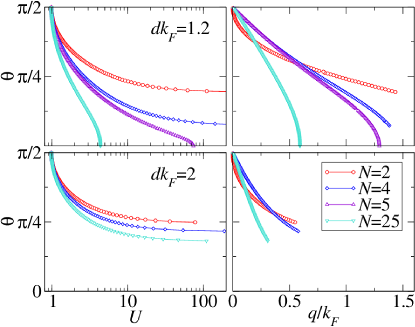
Figure 5: (Color online) Phase boundaries (left panels) and rescaled stripe wavevector at the boundaries $q_{c}/k_{F}$ (right panels) for the $\varphi=0$ stripe phase for different values of the number of layers $N$ and two fixed values of the layer distance: $dk_{F}=1.2$ (top panels) and $dk_{F}=2$ (bottom panels).

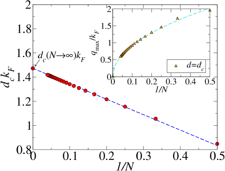
Figure 6: (Color online) Critical value of the interlayer distance $d_{c}k_{F}$ at which $\theta_{c}=0$ (at $U\to\infty$) as a function of the inverse number of layers, $1/N$. In the limit $N\to\infty$, $d_{c}k_{F}=1.47$. Numerical data are represented as (red) circles, while the dashed (blue) line is a linear fit to the data. Inset: maximum value of the stripe wavevector $q_{c}/k_{F}$ for $d=d_{c}$ as a function of $1/N$. Data are (orange) triangles, while the (turquoise) dashed line is a non-linear fit giving $f(1/N)=2.83(1/N)^{0.49}$.

To gain insight into the phase diagram of the multilayer system, we first focus on the trilayer $N=3$. In Fig. 4, we plot the phase boundaries for the instability to a $\varphi=0$ stripe phase (left panel) and the associated critical wavevectors $q_{c}/k_{F}$ (right panel) for different values of the layer distance $dk_{F}$. The qualitative behaviour we observe here is common to any number of layers $N$, including the case of a bilayer $N=2$. For large enough layer distance $d$, the $\varphi=0$ stripe phase can only occur for values of the tilt angle greater than a critical angle $\theta_{c}$, i.e., at the stripe instability boundary, we have $U\to\infty$ for $\theta\to\theta_{c}$ ([green] circle symbols). However, when the layer distance decreases, we find that $\theta_{c}$ eventually reaches zero at a critical distance $d_{c}$ ([violet] star symbols): Here, the $\varphi=0$ stripe phase spans the entire range of tilt angles $\theta$. For smaller distances, $d<d_{c}$, stripe formation is always possible for sufficiently large but finite values of the interaction strength $U$, even for dipoles aligned perpendicular to the planes.

Note that when decreasing the value of $dk_{F}$, eventually our exchange-only formalism becomes questionable, since it neglects interlayer correlations. In fact, for $k_{F}d\lesssim 1$, interlayer pairing (e.g., dimers in the two-layer configuration Volosniev et al. (2011) and bound chains in multilayers Volosniev et al. (2013)) is expected to dominate over stripe formation, and this is not included in our approximation scheme.

We then investigate whether, by fixing the layer distance to a value $k_{F}d>1$, the $\varphi=0$ stripe phase can dominate the phase diagram as the number of layers $N$ is increased. To this end, we plot in Fig. 5 the phase boundaries (left panels) for the $\varphi=0$ stripe phase for different values of $N$. We observe qualitatively different behaviour depending on whether the distance $d$ is above or below $\sim 1.47/k_{F}$, corresponding to the critical distance $d_{c}$ for $N\to\infty$, as derived in Sec. V. When $d>d_{c}(N\to\infty)$ (lower panels of Fig. 5), the $\varphi=0$ stripe phase exists for an increasingly larger range of dipole tilt angles as $N$ increases, but the critical angle $\theta_{c}$ finally saturates to a finite positive value. When instead $d<d_{c}(N\to\infty)$ (upper panels of Fig. 5), the stripe phase eventually spans the full range of angles, including the situation where the dipole moments are aligned perpendicular to the planes.

These results are summarized in Fig. 6, where we plot, as a function of $1/N$, the critical value of the interlayer distance $d_{c}k_{F}$ at which the $\varphi=0$ stripe phase first spans the full range of dipole tilt angles. The data for $N\to\infty$ in the figures are evaluated following the procedure explained in the next section.

V The $N\to\infty$ limit

We now show how the calculation for the $\varphi=0$ stripe instability can be extended to the limit of an infinite number of layers. The key point is that the interlayer interaction potential $v_{jl}({\mathbf{q}})$ only depends on the layer index difference $|j-l|$, so that, for a system with periodic boundary conditions and $N\gg 1$, we can make a transformation from the layer index space $j=1,2,\dots,N$ to the reciprocal space $p=2\pi m/N$, where $m=-N/2,\ldots,N/2$ Świerkowski et al. (1991):

$$\tilde{u}_{p}=\sum_{j-l=-N}^{N}e^{-i(j-l)p}v_{jl}\;.$$ (16)

Of course, in the actual system, we do not have periodic boundary conditions, but this should not change the physics in the limit $N\to\infty$. Inserting Eq. (2) yields the analytical solution

$$\tilde{u}_{p}({\mathbf{q}})=-2\pi D^{2}q\left[\frac{\zeta(\theta,\varphi)}{e^{ip+qd}-1}+\frac{\zeta(\theta,\varphi+\pi)}{e^{-ip+qd}-1}\right]\;,$$ (17)

where $\zeta(\theta,\varphi)=\xi(\theta,\varphi)+i\sin 2\theta\cos\varphi$, and where we have taken the limit $N\to\infty$ after evaluating the geometric series.

We thus obtain the following expression for the eigenvalues of the inverse density-density response function:

$$\tilde{\chi}^{-1}_{p}({\mathbf{q}},\omega)=\frac{1}{\Pi({\mathbf{q}},\omega)}-v({\mathbf{q}})[1-G({\mathbf{q}})]-\tilde{u}_{p}({\mathbf{q}})\;.$$ (18)

To investigate the instabilities, we take the static limit, $\omega=0$, and determine the values of $p$ and ${\mathbf{q}}$ for which $\tilde{\chi}^{-1}_{p}$ first hits zero. In practice, this means we must find the value of $p$ that maximizes $-\tilde{u}_{p}({\mathbf{q}})$ for each ${\mathbf{q}}$. Solving for the stationary points gives us two solutions:

$$p_{i=1,2}=2\arctan\left[\frac{\left(e^{qd}\mp 1\right)\sin\theta\cos\varphi}{\left(e^{qd}\pm 1\right)\cos\theta}\right]+\pi\delta_{i,2}\;,$$ (19)

where the argument is positive if we assume $0\leq\varphi\leq\pi/2$. The first solution $p_{1}$ corresponds to the maximum of $-\tilde{u}_{p}({\mathbf{q}})$, where we have

$$\tilde{u}_{p_{1}}({\mathbf{q}})=-4\pi D^{2}q\left(\frac{\cos^{2}\theta}{e^{qd}-1}-\frac{\cos^{2}\varphi\sin^{2}\theta}{e^{qd}+1}\right)\;.$$ (20)

Thus we have now considerably simplified the problem, as we only have to find the zero of the maximum inverse eigenvalue of the static response, $\tilde{\chi}^{-1}_{p_{1}}({\mathbf{q}},0)$, as a function of ${\mathbf{q}}$.

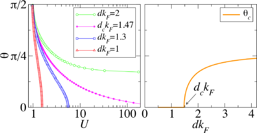
Figure 7: (Color online) Left panel: Phase boundary of the collapsed region for an infinite number of layers $N\to\infty$ and different values of the rescaled layer density $dk_{F}$. The instability to collapse is signalled by an infinite compressibility of the dipolar gas, i.e., by a divergence of the static response function for ${\mathbf{q}}_{c}=0$. While for $d>d_{c}$, collapse occurs only for a tilt angle larger than a critical value $\theta_{c}$, for $d<d_{c}$, the collapsed phase spans the entire range of angles. Right panel: We plot the asymptotic values of the tilt angle at the phase boundary for $U\to\infty$, $\theta_{c}$, as a function of the rescaled layer distance $dk_{F}$; we find that the critical distance for infinite layers is given by $d_{c}(N\to\infty)k_{F}=1.47$.

In this limit, we always find that $(q_{c},\varphi_{c})=0$, i.e., by increasing the number of layers to infinity, the gas becomes unstable towards mechanical collapse. Here, the gas compressibility, which is proportional to the static response function at ${\mathbf{q}}=0$, is infinite. The results for the phase boundary of such a collapsed phase are summarized in Fig. 7 and are qualitatively similar to the boundaries found for the $\varphi=0$ stripe phase in the case of a finite number of layers. Below the critical layer distance $d_{c}k_{F}\simeq 1.47$, the collapsed phase exists for any value of the dipole tilt angle, including $\theta=0$.

The behaviour of the infinite $N$ multilayer system is reminiscent of that expected for the 3D dipolar Fermi gas, where one also has collapse for sufficiently large dipolar interactions Sogo et al. (2009). In particular, the $\theta=0$ case possesses the same rotational symmetry as the 3D gas with aligned dipole moments. Therefore, it is instructive to compare the onset of collapse for $\theta=0$ in the multilayer system to that in the 3D case. First, one can define a 3D density for the multilayer geometry:

$$n_{\text{3D}}=\frac{n}{d}=\frac{k_{F}^{3}}{4\pi(k_{F}d)}\;.$$ (21)

This then yields the corresponding 3D dimensionless interaction parameter:

$$U_{\text{3D}}\equiv\frac{mD^{2}}{\hbar^{2}}n_{\text{3D}}^{1/3}=\frac{U}{(4\pi k_{F}d)^{1/3}}\;.$$ (22)

In the 3D dipolar gas, the collapse instability occurs at $U_{\text{3D}}\simeq 2.4$ Sogo et al. (2009). Thus, to obtain a comparable $U_{\text{3D}}$ for collapse in the multilayer system, we require $dk_{F}\simeq 1.31$ and $U\simeq 6.12$. In our 2D infinite layer configuration, we can interpret the parameter $dk_{F}$ as an effective Fermi surface “deformation” parameter if we treat $2\pi/d$ as a Fermi momentum in the $z$ direction. This assumes that it is the inter-particle spacing rather the fermion exchange that is the key feature of the Fermi surface deformation in 3D when considering the collapse instability. For the multilayer geometry, the ratio between the Fermi momenta in the $z$ and radial directions is then given by $2\pi/(k_{F}d)$, thus yielding $k_{F,z}/k_{F,r}\sim 4.8$ at the collapse instability. This is not so dissimilar from that obtained for the 3D Fermi gas within Hartree-Fock mean-field theory, where $k_{F,z}/k_{F,r}\sim 2$ Sogo et al. (2009). In the layered system, we can effectively tune the deformation such that the critical $U_{\text{3D}}$ for collapse is raised (lowered) by increasing (decreasing) $dk_{F}$. Eventually, when $d>d_{c}$, the Fermi surface is not sufficiently elongated along the dipole direction to produce collapse.

VI Concluding remarks

In this work, we have analysed the density instabilities of dipolar Fermi multilayer systems that are driven by the attractive part of the dipolar interaction. We have argued that such instabilities are dominated by exchange correlations and can thus be described using a simplified exchange-only STLS approach. We find that the attraction-driven $\varphi=0$ stripe phase expands to fill the phase diagram with an increasing number of layers $N$. However, at the same time, the stripe wavevector decreases so that the stripe phase is eventually replaced by collapse as $N\to\infty$. For the case $\theta=0$, the infinite $N$ limit resembles a 3D dipolar gas with a Fermi surface deformation that can be tuned by varying the interlayer distance $dk_{F}$.

Our predicted stripe phases should be assessable in experiments on polar molecules with sufficiently large dipole moments. One also needs to consider the issue of losses in experiments when strong interactions are involved. The restricted motion in the 2D geometry reduces the possibility of head-to-tail collisions between dipoles, which underlies the dominant loss process in dipolar gases, but such collisions are not necessarily suppressed when we have a large dipole tilt. However, we expect that chemically stable molecules such as ²³Na⁴⁰K Park et al. (2015) will make it possible to probe this regime of parameter space.

In the future, it would be interesting to extend our results to finite temperature, where the proliferation of topological defects can melt the stripe phase Wu et al. . Furthermore, one could investigate the effects of pairing using more sophisticated approaches to the multilayer system such as the Euler-Lagrange Fermi-hypernetted-chain approximation Abedinpour et al. (2014). Finally, there is the intriguing question of how our predicted phase diagram connects with other instabilities such as nematic phases or collapse within the stripe phase.

Appendix A Non-interacting static structure factor

We start with the general expression for the non-interacting static structure factor in two dimensions Giuliani and Vignale (2005):

$$S^{(0)}({\mathbf{q}})=1-\frac{1}{n}\int\displaystyle\frac{d{\mathbf{k}}}{(2\pi)^{2}}n_{\mathbf{k}}n_{{\mathbf{k}}+{\mathbf{q}}}\;,$$ (23)

where $n$ is the 2D density and $n_{\mathbf{k}}=\Theta(k_{F}-k)$ the zero-temperature Fermi distribution function. Here, the integral simply corresponds to calculating the area $A$ of the overlap region between two identical circles of radius $k_{F}$, as shown in Fig. 8. Due to the symmetry of the problem, we only need to consider half of the overlap region as follows.

Assuming $q<2k_{F}$, we first determine the segment area spanned by the angle $2\theta$ in the left circle of Fig. 8:

$$A_{\rm seg}=k_{F}^{2}\theta$$

where $\cos\theta=q/2k_{F}$. Next, we determine the area of the left triangle obtained by drawing a line through the points where the circles intersect:

$$A_{\Delta}=\frac{1}{2}k_{F}q\sin\theta=\frac{1}{2}k_{F}q\sqrt{1-\left(\frac{q}{2k_{F}}\right)^{2}}$$

Then we obtain:

$$A=2(A_{\rm seg}-A_{\Delta})\\ =2k_{F}^{2}\arccos\left(\frac{q}{2k_{F}}\right)-k_{F}q\sqrt{1-\left(\frac{q}{2k_{F}}\right)^{2}}$$ (24)

Inserting (24) into (23), and using the fact that $\arcsin x=\pi/2-\arccos x$, we finally recover Eq. (6) in the main text.

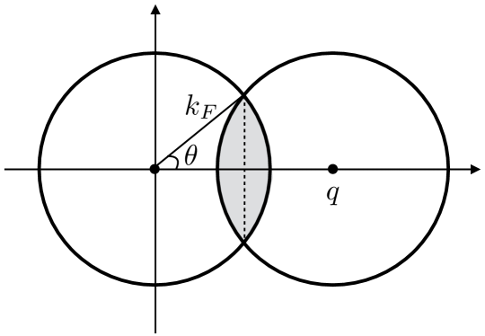
Figure 8: Two identical circles of radius $k_{F}$, where the centers are separated by a distance $q$ in $k$-space. The area of the shaded overlapping region corresponds to the integral in Eq. (23), defining the the non-interacting static structure factor in 2D.

References

- Baranov (2008) M. A. Baranov, Phys. Rep. 464, 71 (2008).
- Lahaye et al. (2009) T. Lahaye, C. Menotti, L. Santos, M. Lewenstein, and T. Pfau, Rep. Prog. Phys. 72, 126401 (2009).
- Baranov et al. (2012) M. A. Baranov, M. Dalmonte, G. Pupillo, and P. Zoller, Chemical Reviews 112, 5012 (2012).
- Grüner (1988) G. Grüner, Rev. Mod. Phys. 60, 1129 (1988).
- Kivelson et al. (1998) S. A. Kivelson, E. Fradkin, and V. J. Emery, Nature 393, 550 (1998).
- Kivelson et al. (2003) S. A. Kivelson, I. P. Bindloss, E. Fradkin, V. Oganesyan, J. M. Tranquada, A. Kapitulnik, and C. Howald, Rev. Mod. Phys. 75, 1201 (2003).
- Naylor et al. (2015) B. Naylor, A. Reigue, E. Maréchal, O. Gorceix, B. Laburthe-Tolra, and L. Vernac, Phys. Rev. A 91, 011603 (2015).
- Lu et al. (2012) M. Lu, N. Q. Burdick, and B. L. Lev, Phys. Rev. Lett. 108, 215301 (2012).
- Aikawa et al. (2014a) K. Aikawa, A. Frisch, M. Mark, S. Baier, R. Grimm, and F. Ferlaino, Phys. Rev. Lett. 112, 010404 (2014a).
- Aikawa et al. (2014b) K. Aikawa, S. Baier, A. Frisch, M. Mark, C. Ravensbergen, and F. Ferlaino, Science 345, 1484 (2014b).
- Carr et al. (2009) L. D. Carr, D. DeMille, R. V. Krems, and J. Ye, New J. Phys. 11, 055049 (2009).
- Ni et al. (2008) K. K. Ni, S. Ospelkaus, M. H. G. De Miranda, A. Pe’er, B. Neyenhuis, J. J. Zirbel, S. Kotochigova, P. S. Julienne, D. S. Jin, and J. Ye, Science 322, 231 (2008).
- Ospelkaus et al. (2010) S. Ospelkaus, K.-K. Ni, D. Wang, M. H. G. de Miranda, B. Neyenhuis, G. Quéméner, P. S. Julienne, J. L. Bohn, D. S. Jin, and J. Ye, Science 327, 853 (2010).
- Ni et al. (2010) K. K. Ni, S. Ospelkaus, M. H. G. De Miranda, A. Pe’er, B. Neyenhuis, J. J. Zirbel, S. Kotochigova, P. S. Julienne, D. S. Jin, and J. Ye, Nature 464, 1324 (2010).
- Heo et al. (2012) M.-S. Heo, T. T. Wang, C. A. Christensen, T. M. Rvachov, D. A. Cotta, J.-H. Choi, Y.-R. Lee, and W. Ketterle, Phys. Rev. A 86, 021602 (2012).
- Repp et al. (2013) M. Repp, R. Pires, J. Ulmanis, R. Heck, E. D. Kuhnle, M. Weidemüller, and E. Tiemann, Phys. Rev. A 87, 010701 (2013).
- Wu et al. (2012) C.-H. Wu, J. W. Park, P. Ahmadi, S. Will, and M. W. Zwierlein, Phys. Rev. Lett. 109, 085301 (2012).
- Park et al. (2015) J. W. Park, S. A. Will, and M. W. Zwierlein, Phys. Rev. Lett. 114, 205302 (2015).
- de Miranda et al. (2011) M. H. G. de Miranda, A. Chotia, B. Neyenhuis, D. Wang, G. Quéméner, S. Ospelkaus, J. L. Bohn, J. Ye, and D. S. Jin, Nature Phys. 7, 502 (2011).
- Miyakawa et al. (2008) T. Miyakawa, T. Sogo, and H. Pu, Phys. Rev. A 77, 061603 (2008).
- Sogo et al. (2009) T. Sogo, L. He, T. Miyakawa, S. Yi, H. Lu, and H. Pu, New Journal of Physics 11, 055017 (2009).
- Endo et al. (2010) Y. Endo, T. Miyakawa, and T. Nikuni, Phys. Rev. A 81, 063624 (2010).
- Zhang and Yi (2009) J.-N. Zhang and S. Yi, Phys. Rev. A 80, 053614 (2009).
- Zhang and Yi (2010) J.-N. Zhang and S. Yi, Phys. Rev. A 81, 033617 (2010).
- Krieg et al. (2015) J. Krieg, P. Lange, L. Bartosch, and P. Kopietz, Phys. Rev. A 91, 023612 (2015).
- Baillie et al. (2015) D. Baillie, R. N. Bisset, and P. B. Blakie, Phys. Rev. A 91, 013613 (2015).
- Lu and Shlyapnikov (2012) Z.-K. Lu and G. V. Shlyapnikov, Phys. Rev. A 85, 023614 (2012).
- Yamaguchi et al. (2010) Y. Yamaguchi, T. Sogo, T. Ito, and T. Miyakawa, Phys. Rev. A 82, 013643 (2010).
- Sun et al. (2010) K. Sun, C. Wu, and S. Das Sarma, Phys. Rev. B 82, 075105 (2010).
- Babadi and Demler (2011) M. Babadi and E. Demler, Phys. Rev. B 84, 235124 (2011).
- Sieberer and Baranov (2011) L. M. Sieberer and M. A. Baranov, Phys. Rev. A 84, 063633 (2011).
- Parish and Marchetti (2012) M. M. Parish and F. M. Marchetti, Phys. Rev. Lett. 108, 145304 (2012).
- van Zyl et al. (2015) B. P. van Zyl, W. Kirkby, and W. Ferguson, Phys. Rev. A 92, 023614 (2015).
- Matveeva and Giorgini (2012) N. Matveeva and S. Giorgini, Phys. Rev. Lett. 109, 200401 (2012).
- Bruun and Taylor (2008) G. M. Bruun and E. Taylor, Phys. Rev. Lett. 101, 245301 (2008).
- Wu et al. (2015) Z. Wu, J. K. Block, and G. M. Bruun, Phys. Rev. B 91, 224504 (2015).
- Block and Bruun (2014) J. K. Block and G. M. Bruun, Phys. Rev. B 90, 155102 (2014).
- Marchetti and Parish (2013) F. M. Marchetti and M. M. Parish, Phys. Rev. B 87, 045110 (2013).
- Singwi et al. (1968) K. S. Singwi, M. P. Tosi, R. H. Land, and A. Sjölander, Phys. Rev. 176, 589 (1968).
- Pikovski et al. (2010) A. Pikovski, M. Klawunn, G. V. Shlyapnikov, and L. Santos, Phys. Rev. Lett. 105, 215302 (2010).
- Matveeva and Giorgini (2014) N. Matveeva and S. Giorgini, Phys. Rev. A 90, 053620 (2014).
- Block et al. (2012) J. K. Block, N. T. Zinner, and G. M. Bruun, New J. Phys. 14, 105006 (2012).
- Fischer (2006) U. R. Fischer, Phys. Rev. A 73, 031602 (2006).
- Li et al. (2010) Q. Li, E. H. Hwang, and S. Das Sarma, Phys. Rev. B 82, 235126 (2010).
- Zheng and MacDonald (1994) L. Zheng and A. H. MacDonald, Phys. Rev. B 49, 5522 (1994).
- Giuliani and Vignale (2005) G. F. Giuliani and G. Vignale, Quantum Theory of the Electron Liquid (Cambridge University Press, 2005).
- Stern (1967) F. Stern, Phys. Rev. Lett. 18, 546 (1967).
- Volosniev et al. (2011) A. G. Volosniev, N. T. Zinner, D. V. Fedorov, A. S. Jensen, and B. Wunsch, J. Phys. B: At. Mol. Opt. Phys. 44, 125301 (2011).
- Volosniev et al. (2013) A. Volosniev, J. Armstrong, D. Fedorov, A. Jensen, and N. Zinner, Few-Body Systems 54, 707 (2013).
- Świerkowski et al. (1991) L. Świerkowski, D. Neilson, and J. Szymański, Phys. Rev. Lett. 67, 240 (1991).
- (51) Z. Wu, J. K. Block, and G. M. Bruun, “Liquid crystal phases of two-dimensional dipolar gases and berezinskii-kosterlitz-thouless melting,” ArXiv:1509.02679.
- Abedinpour et al. (2014) S. H. Abedinpour, R. Asgari, B. Tanatar, and M. Polini, Annals of Physics 340, 25 (2014).