Relaxation of nonspherical sessile drops towards equilibrium

Abstract

We present a theoretical study related to a recent experiment on the coalescence of sessile drops. The study deals with the kinetics of relaxation towards equilibrium, under the action of surface tension, of a spheroidal drop on a flat surface. For such a non-spherical drop under partial wetting conditions, the dynamic contact angle varies along the contact line. We propose a new non-local approach to the wetting dynamics, where the contact line velocity depends on the geometry of the whole drop. We compare our results to those of the conventional approach in which the contact line velocity depends only on the local value of the dynamic contact angle. The influence on drop dynamics of the pinning of the contact line by surface defects is also discussed.

I Introduction

At first glance, the motion of the gas-liquid interface along the solid surface is a purely hydrodynamic problem. However, it attracted significant attention from the physicists since the work Huh , which showed an unphysical divergence that appears in the hydrodynamic treatment if a motion of a wedge-shaped liquid slides along the solid surface. The reason for this divergence lies in the no-slip condition (i.e. zero liquid velocity) at the solid surface. Being so common in hydrodynamics, this boundary condition is questionable in the vicinity of the contact line along which the gas-liquid interface joins the solid. In the absence of mass transfer between the gas and the liquid, the no-slip condition requires zero velocity for the contact line that is supposed to be formed of the liquid molecules in the contact with the solid. It means that, for example, an oil drop cannot move along the glass because of the no-slip condition! Of course, this contradicts the observations.

The experiment Duss demonstrated that the velocity on the liquid-gas interface is directed towards the contact line during the contact line advance. The authors interpreted this result by the rolling (”caterpillar”) motion of the drop footnote . However, later theoretical study Mahad shows that such a motion is compatible with the no-slip condition on the non-deformable solid surface only for the contact angles close to $180^{\circ}$.

The justification of the no-slip condition is well known DeGennes : it is the excess of the attractive force between the solid and the liquid molecules over the force between two liquid molecules. This attraction has a tendency to prevent the motion of the liquid molecules adjacent to the solid. Obviously, the same forces resist when these molecules are forced to move. In other words, some relatively large (with respect to viscous dissipation) energy should be spent for this forcing.

Numerous microscopic theories (see e.g. DeGennes ; CoalP ; Sh ; Sepp ; YP ; Cox ; Voi ; Blake ) propose different phenomena as to be responsible for the contact line motion. However, no general theory has been agreed upon. This situation is partly due to the scarceness of the information that can be extracted from the experiments. Most of them deal with either drops with cylindrical symmetry (circular contact lines) or the climbing of the contact line over a solid immersed into a liquid (straight contact line). In these experiments, the contact line velocity $v_{n}$ measured in the normal direction does not vary along the contact line on a macroscopic scale larger than the size of the surface defects. The experiments with non-spherical drops where such a variation exists can give additional information. This information can be used to test microscopic models of the contact line motion. To our knowledge, there are only two kinds of investigated situations that feature the non-spherical drops. The first one is the sliding of the drop along an inclined surface sliding . The second concerns the relaxation of the sessile drops of complicated shape towards the equilibrium shape of spherical cap. This latter case was studied experimentally in CoalP for water drops on the silanized silicon wafers at room temperature. The present article deals with this second case.

The principal results of CoalP can be summarized as follows:

(i) The relaxation of the drop from the elongated shape towards the spherical shape is exponential. The characteristic relaxation time $\tau$ is proportional to the drop size. The drop size can be characterized by the contact line radius $R^{\ast}$ at equilibrium when the drop eventually relaxes towards a spherical cap.

(ii) The dependence of $\tau$ on the equilibrium contact angle $\theta$ is not monotonous: $\tau(30^{\circ})<\tau(53^{\circ})$ and $\tau(53^{\circ})>\tau(70^{\circ})$.

(iii) The relaxation is extremely slow. The capillary number $Ca=R^{\ast}\eta/(\tau\sigma)$ is of the order of $10^{-7}$, where $\sigma$ is the surface tension and $\eta$ is the shear viscosity.

Since the motion is not externally forced, a small $Ca$ shows that the energy dissipated in the vicinity of the contact line is much larger than in the bulk of the drop.

The contact line motion is characterized by the normal component $v_{n}$ of its velocity. Many existing theories result in the following relationship between $v_{n}$ and the dynamic contact angle $\theta$:

$$v_{n}=v_{c}\,F(\theta,\theta_{s}),$$ (1)

where $\theta_{s}$ is the static contact angle, $v_{c}$ is a constant characteristic velocity and $F$ is a function of two arguments, the form of which depends on the model used. For all existing models, the following relation is satisfied

$$F(\theta,\theta_{s})=-F(\theta_{s},\theta),$$ (2)

which implies the trivial condition $F(\theta_{s},\theta_{s})=0$. It means simply that the line is immobile when $\theta=\theta_{s}$.

The theories of Voinov Voi and Cox Cox correspond to

$$F=\theta^{3}-\theta_{s}^{3}.$$ (3)

There are many theories (see e.g. DeGennes , Sh ) which result in

$$F=\cos\theta_{s}-\cos\theta.$$ (4)

In a recent model by Pomeau CoalP ; YP , it is proposed that

$$F=\theta-\theta_{s}$$ (5)

with the coefficient $v_{c}$ that depends on the direction of motion (advancing or receding) but not on the amplitude of $v_{n}$.

Since the drop evolution is extremely slow, the drop shape can be calculated using the quasi-static argument according to which at each moment the drop surface can be calculated from the constant curvature condition and the known position of the contact line. The major problem is how to find this position. Independently of the particular contact line motion mechanism, at least two approaches are possible. The first of them is the “local” approach CoalP , which consists in the determination of the position of a given point of the contact line from Eq. (1) where $\theta$ is assumed to be the local value of the dynamic contact angle at this point. Another, non-local approach is suggested in sec. II. Certainly, both of this approaches should give the same result when $v_{n}$ does not vary along the contact line. However, we show that the result is different in the opposite case.

The influence of surface defects on the contact line dynamics is considered in sec. III.

II Nonlocal approach to the contact line dynamics

In this section we generalize another approach, suggested in DeCon , for an arbitrary drop shape. This approach postulates neither Eq. (1) nor a particular line motion mechanism. It simply assumes that the energy dissipated during the contact line motion is proportional to its length and does not depend on the direction of motion (advancing or receding). Then, at low contact line velocity, the leading contribution to the energy dissipated per unit time (i.e. the dissipation function) can be written in the form

$$T=\oint{\xi\,v_{n}^{2}\over 2}\;{\rm d}l,$$ (6)

where the integration is performed over the contact line and $\xi$ is the constant dissipation coefficient. According to the earlier discussed experimental results CoalP , the dissipation in the bulk is assumed to be much smaller than that in the vicinity of the contact line.

Since we assume that most dissipation takes place in the region of the drop adjacent to the contact line, our discussion is limited to the case where the prewetting film (that is observed for zero or very low contact angles) is absent. This situation corresponds to the conditions of the experiment CoalP where the dropwise (as opposed to filmwise) condensation shows the absence of the prewetting liquid film. The above assumption also limits the description to the partial wetting case. This assumption is also justified by the experimental conditions under which it is extremely difficult to obtain macroscopic convex drops for the contact angles $<30^{\circ}$ because of the contact line pinning CoalP . The main reason is that the potential energy $U$ of the drop from Eq. (46) goes to zero as the contact angle goes to zero. At small contact angles $U$ is not large enough to overcome the pinning forces that originate from the surface defects, see sec. III. Therefore, the macroscopic convex drops under consideration can not be observed at small contact angles.

Generally speaking, the behavior of the drop obeys the Lagrange equation Land

$${{\rm d}\over{\rm d}t}\left({\partial{\cal L}\over\partial\dot{q_{j}}}\right)-{\partial{\cal L}\over\partial q_{j}}=-{\partial T\over\partial\dot{q_{j}}},$$ (7)

where the Lagrangian ${\cal L}=K-U$ is the function of the generalized coordinates $q_{j}$ and of their time derivatives which are denoted by a dot. The current time is denoted by $t$, $K$ is the kinetic energy, and $U=U(q_{j})$ is the potential energy. Since there is no externally forced liquid motion in this problem and the drop shape change is extremely slow, we can neglect the kinetic energy by putting ${\cal L}=-U$. Then Eq. (7) reduces to

$${\partial U\over\partial q_{j}}=-{\partial T\over\partial\dot{q_{j}}},$$ (8)

the expression applied first to the contact line motion in DeGennes .

The potential energy of a sessile drop is DeCon

$$U=\sigma(A_{VL}-A_{SL}\cos\theta_{eq}),$$ (9)

where $\sigma$ is the liquid surface tension, $A_{VL}$ and $A_{LS}$ are the areas of the vapor-liquid and liquid-solid interfaces respectively and $\theta_{eq}$ is the equilibrium value of the contact angle. We neglect the contribution due to the van der Waals forces because we consider macroscopic drops and large contact angles $\geq 30^{\circ}$. For such drops the van der Waals forces influence the interface shape only in the very close vicinity of the contact line and this influence can be neglected.

In general the static contact angle $\theta_{s}$ is not equal to $\theta_{eq}$ because of the presence of the defects, a problem which will be treated in the section III. Meanwhile, we assume that $\theta_{s}=\theta_{eq}$. The gravitational contribution is neglected in Eq. (9) because the drops under consideration are supposed to be small, with the radius much smaller than the capillary length. The volume of a sessile drop is fixed. Its calculation provides us with another equation, which closes the problem provided that the shape of the drop surface is known. The drop shape is determined from the condition of the quasi-equilibrium which results in the constant curvature of the drop surface.

Usually, the wetting dynamics is observed either for the spreading of droplets with the shape of the spherical cap, or for the motion of the liquid meniscus in a cylindrical capillary, or for the extraction of a solid plate from the liquid DeGennes . In all these cases, the contact line velocity $v_{n}$ does not vary along the contact line and the dissipation function in the form Eq. (6) results in the expression DeCon

$$v_{n}={\sigma\over\xi}\,(\cos\theta_{s}-\cos\theta),$$ (10)

which is equivalent to Eq. (1), with the function $F$ taking the usual form (4). One might think that this equivalence confirms the universal nature of this expression. In the next section we show that it is not exactly so because the non-local approach results in a different expression when $v_{n}$ varies along the contact line.

Let us now apply the algorithm described above to the problem of drop relaxation. A shape for a non-spherical drop surface of constant curvature can be found only numerically. In order to treat the problem analytically, we approximate the drop shape by a spheroidal cap that is described in Cartesian $(x,y,z)$ coordinate system by the equation

$${\frac{x^{2}}{a^{2}}}+{\frac{y^{2}+(z+d)^{2}}{b^{2}}}=1$$ (11)

at $z>0$, the plane XOY corresponding to the solid surface. The symmetry of the problem allows only quarter of the drop (see Fig. 1) to be considered.

Figure 1: Reference system to describe the 3D spheroidal cap. Only one quarter of it is shown. The surface is described by Eq. 11. The local contact angles at the points M and N are shown too.

Since one of the parameters $(a,b,d)$ is fixed by the condition of the conservation of the drop volume that can be calculated as

$$V={\frac{\pi}{3}}{\frac{a}{b}}\,(2\,b^{3}-3\,b^{2}d+d^{3}),$$ (12)

there are only two free parameters left.

The time-dependent parameters $a$ and $b$ can be taken as generalized coordinates. However, it is more convenient to use another set of parameters, $R_{x}$ and $R_{y}$, which are the half-axes of the ellipse that form the base of the drop (see Fig. 1), $R_{y}>R_{x}$. They are related to $a$ and $b$ by the equations

$$R_{y}^{2}+d^{2}=b^{2},\quad\mbox{and}\quad R_{x}b=R_{y}a,$$ (13)

that follow from Eq. (11). At the end of the relaxation

$$R_{x}=R_{y}=R\sin\theta_{s}\equiv R^{\ast},$$ (14)

where $R$ is the final radius of curvature of the drop. Therefore, during the late stage

$$\begin{array}[]{l}R_{x}=R^{\ast}\,(1-r_{x})\\ R_{y}=R^{\ast}\,(1+r_{y})\end{array}$$ (15)

with $|r_{x,y}|\ll 1$. Some points of the contact line advance, some points recede. The dynamic contact angle changes its value along the contact line. In particular, the point N$(R_{x},0,0)$ in Fig. 1 advance and M$(0,R_{y},0)$ recede. These points are extreme and their velocities have the maximum absolute values, positive for N and negative for M. The dynamic contact angles ($\theta_{da}$: dynamic advancing contact angle in N and $\theta_{dr}$: dynamic receding contact angle in M) also have the extreme values there. They can be found from the equations

$$\begin{array}[]{l}\cos\theta_{dr}=d/b,\\ \tan\theta_{da}=R_{y}^{2}\,/(d\,R_{x}),\end{array}$$ (16)

that reduce for $r_{x},r_{y}\ll 1$ to

$$\begin{array}[]{r}\cos\theta_{dr}=\cos\theta_{s}+\sin^{2}\theta_{s}(2+\cos\theta_{s})\cdot\\ (2\,r_{y}-r_{x})/3,\\ \cos\theta_{da}=\cos\theta_{s}-\sin^{2}\theta_{s}\,[(2+4\,\cos\theta_{s})\,r_{x}-\\ (4-\cos\theta_{s})\,r_{y}]/3.\end{array}$$ (17)

Eq. 8, written for the generalized coordinates $r_{x}$ and $r_{y}$ together with the expression for the dissipation function (see Appendix A), implies the set of equations

$$\left\{\begin{array}[]{c}3\,\dot{r}_{x}-\dot{r}_{y}=\tau_{0}^{-1}(B\,r_{y}-A\,r_{x}),\\ 3\,\dot{r}_{y}-\dot{r}_{x}=\tau_{0}^{-1}(B\,r_{x}-A\,r_{y}),\end{array}\right.$$ (18)

where $\tau_{0}=\sigma R^{\ast}/\xi$ and the coefficients $A$ and $B$ are given by Eq. (47) in Appendix A. The solutions of Eqs. 18 read

$$r_{x}(t)=[(r_{x}^{(i)}-r_{y}^{(i)})\,\exp(-t/\tau_{s})+$$

$$(r_{x}^{(i)}+r_{y}^{(i)})\,\exp(-t/\tau_{n})]/2,$$ (19)

$$r_{y}(t)=[(r_{y}^{(i)}-r_{x}^{(i)})\,\exp(-t/\tau_{s})+$$

$$(r_{x}^{(i)}+r_{y}^{(i)})\,\exp(-t/\tau_{n})]/2,$$ (20)

where $r_{x}^{(i)}$ and $r_{y}^{(i)}$ are the initial ($t=0$) values for $r_{x}$ and $r_{y}$ respectively, and the relaxation times

$$\tau_{s}=\tau_{0}/[\sin^{2}\theta_{s}\,(2+\cos\theta_{s})],$$ (21)

$$\tau_{n}=45\,\tau_{0}\,(1+\cos\theta_{s})/[(108+41\,\cos\theta_{s}+$$

$$14\,\cos^{2}\theta_{s}+17\,\cos^{3}\theta_{s})(1-\cos\theta_{s})].$$ (22)

The variables $r_{x}$ and $r_{y}$ are defined in Eq. (15) in such a way that when $r_{x}^{(i)}=-r_{y}^{(i)}$ the drop surface remains spherical during its relaxation. One can see from Eqs. (19,20) that the evolution is defined entirely by the characteristic time $\tau_{s}$ (“spherical”) in this case. When $r_{x}^{(i)}=r_{y}^{(i)}$, only $\tau_{n}$ (“non-spherical”) defines the drop evolution. In the real experimental situation where $(r_{x}^{(i)}-r_{y}^{(i)})\ll(r_{x}^{(i)}+r_{y}^{(i)})$, the relaxation time $\tau_{n}$ alone defines the relaxation of the drop as it follows from Eqs. (19, 20). Therefore $\tau_{n}$ should be associated with the experimentally observed relaxation time.

The functions $\tau_{s,n}(\theta_{s})$ are plotted in Fig. 2 assuming that $\xi$ is independent of $\theta_{s}$.

Figure 2: The relaxation times $\tau_{s,n}$ versus the static contact angle $\theta_{s}$.

Clearly, both $\tau_{s}$ and $\tau_{n}$ increase monotonically with $\theta_{s}$ in agreement with the observed tendency for large contact angles.

It is interesting to check whether or not by applying the local approach of Eq. (10) we recover the non-local result for $v_{n}$. This is easy to do for the case $r_{x}^{(i)}=r_{y}^{(i)}$, i.e. when $r_{x}=r_{y}$. In this case, the non-local model (18) implies $\dot{r}_{x}=-r_{x}/\tau_{n}$, and the contact line velocities at the points M and N are

$$v_{n}= -{\sigma\over\xi}{\tau_{0}\over\tau_{n}}\,r_{x}\quad\mbox{at the point M,}$$ (23)

$$v_{n}= {\sigma\over\xi}{\tau_{0}\over\tau_{n}}\,r_{x}\quad\mbox{at the point N.}$$ (24)

Since Eq. (17) results in

$$(\cos\theta_{s}-\cos\theta)=-\sin^{2}\theta_{s}\,(2+$$

$$\cos\theta_{s})\,r_{x}/3\;\mbox{at the point M,}$$ (25)

$$(\cos\theta_{s}-\cos\theta)=\sin^{2}\theta_{s}\,(5\,\cos\theta_{s}-$$

$$2)\,r_{x}/3\;\mbox{at the point N,}$$ (26)

the local approach (10) implies that

$$v_{n}= -{\sigma\over\xi}{1\over 3}\sin^{2}\theta_{s}\,(2+\cos\theta_{s})\,r_{x}\quad\mbox{at the point M,}$$ (27)

$$v_{n}= {\sigma\over\xi}{1\over 3}\sin^{2}\theta_{s}\,(5\,\cos\theta_{s}-2)\,r_{x}\quad\mbox{at the point N.}$$ (28)

The comparison of Eqs. (22-24) with Eqs. (27,28) show that the results of the local and the non-local approaches are different. However, one can verify that the results are the same in the limit of very small $\theta_{s}$. For finite contact angles, the non-local approach is not equivalent to the local approach. The main difference can be summarized as follows. The $v_{n}$ value that is obtained with our non-local approach can be presented in the form (1) common for the local approach. However, while the characteristic velocity $v_{c}$ from Eq. (1) is constant in the local approach, it is a function of the position on the contact line in the non-local approach. Indeed, the comparison of Eqs. (23-26) with Eqs. (1, 4) shows that

$$v_{c}= 3\,{\sigma\over\xi}{\tau_{0}\over\tau_{n}}/[\sin^{2}\theta_{s}\,(2+\cos\theta_{s})]\;\mbox{at the point M,}$$ (29)

$$v_{c}= 3\,{\sigma\over\xi}{\tau_{0}\over\tau_{n}}/[\sin^{2}\theta_{s}\,(5\,\cos\theta_{s}-2)]\;\mbox{at the point N.}$$ (30)

We do not expect our model to be a good description for the contact angles close to $90^{\circ}$. The reason is the limitation of the spheroid model for the drop shape. The spheroidal shape necessarily fixes $\theta_{dr}=90^{\circ}$ when $\theta_{da}=90^{\circ}$ independently of the contact line velocity, which is incorrect. In addition, the spheroid model does not work at all for $\theta_{s}>90^{\circ}$. One needs to find the real shape of the drop (which is defined by constant curvature condition) to overcome these difficulties.

In order to estimate the limiting value for $\theta_{s}$ for which the spheroid model works well we mention that the dynamic advancing and receding contact angles defined by Eq. (17) must satisfy the inequality $\theta_{dr}\leq\theta_{s}\leq\theta_{da}$. By putting $r_{x}^{(i)}=r_{y}^{(i)}$ in Eqs. (19, 20) one finds that this inequality is satisfied when $\theta_{s}<66^{\circ}$. The last inequality provides us with the limit of the validity for the spheroidal model.

To conclude this section we note that our non-local approach to the dynamics of wetting is not equivalent to the traditional local approach. Both approaches allow the relaxation time to be calculated for a given contact angle provided that the contact angle dependence of the dissipation coefficient $\xi$ is known. Additional experiments are needed to reveal which approach is the most suitable. Under the assumption that the $\xi(\theta_{s})$ dependence (if any) is weak, we find that the relaxation time decreases with the contact angle.

This result explains the decrease of the relaxation time at large contact angles observed in CoalP . We think that the opposite tendency observed for the small contact angles is related to the influence of the surface addressed in the next section.

III Influence of the surface defects on the relaxation time

The motion of the contact line in the presence of defects has been frequently studied (see DeGennes for a review). However, little is understood at the moment because the problem is very sophisticated. Most of its studies deal with the influence of the defects on the static contact line (see, e. g. Mezard ) when they are responsible for the contact angle hysteresis. The latter was studied in Garoff and Collet for the wedge geometry which assumes the external forcing of the contact line. When the contact line moves under the action of a force $f$, it encounters pinning on the random potential created by surface defects. Thus the motion shows the “stick-slip” behavior. It is characteristic for a wide range of physical systems where pinning takes place and is the basis of the theory of dynamical critical phenomena, in which the average contact line velocity is

$$v_{n}=v_{c}(f/f_{c}-1)^{\beta},$$ (31)

where the exponent $\beta$ is universal and $f_{c}$ is the pinning threshold. This expression is often applied (see Wong and refs. therein) to the contact line motion in the systems, where the geometry of the meniscus does not depend on the dragging force. However, the values of $\beta$ vary widely depending on the experimental conditions and do not correspond to the theoretical predictions. The motion of the contact line during the coalescence of drops is even more complicated because the geometry of the meniscus is constantly changing. Therefore, application of the expression (31) is even more questionable in this situation.

In this section we employ the formalism developed in the previous section in order to understand the influence of the surface defects on the relaxation time of the drop where the contact line is not forced externally. The surface defects are modeled by the spatial variation of the local density of the surface energy, which can be related to the local value of the equilibrium contact angle $\theta_{eq}(\vec{r})$ by the Young formula as was suggested in Garoff to describe the static contact angles. The expression (9) can be rewritten for this case in the form

$$U=\sigma A_{VL}-\sigma\int\limits_{(A_{LS})}\cos\theta_{eq}(\vec{r})\;{\rm d}\vec{r}.$$ (32)

The contribution of the defects and thus the deformation $\delta R_{x}$ of the contact line due to the defects is assumed to be small. Then, in the first approximation that corresponds to the “horizontal averaging” approximation from Garoff

$$U=U^{(0)}+\Delta U.$$ (33)

The superscript $(0)$ means that the corresponding quantity is calculated for $\delta R_{x}=0$ and for the constant value of the contact angle $\bar{\theta}_{eq}$ defined by the expression

$$\bar{\theta}_{eq}=\arccos\left[{\frac{1}{A_{LS}^{(0)}}}\int\limits_{(A_{LS}^{(0)})}\cos\theta_{eq}(\vec{r})\;{\rm d}\vec{r}\right].$$ (34)

Then

$$U^{(0)}=\sigma A_{VL}^{(0)}-\sigma A_{LS}^{(0)}\cos\bar{\theta}_{eq}.$$ (35)

It can be shown that the first-order correction to this value, which appears due to the defects is

$$\Delta U=-\sigma\int\limits_{(A_{LS}^{(0)})}(\cos\theta_{eq}(\vec{r})-\cos\bar{\theta}_{eq})\;{\rm d}\vec{r}.$$ (36)

We accept the following model for defects because it is, on one hand, simple and, on the other hand, proven Garoff to be a good description for the advancing and the receding contact angles in the approximation considered. The defects are supposed to be similar circular spots of radius $r$ arranged in a regular spatially periodic pattern, $\lambda$ being the spatial period, the same in both directions, see Fig. 3.

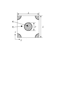
Figure 3: Unit cell of the model defect pattern on the solid surface. The reference system and the values of the contact angle inside the round spots ($\theta_{1}$) and outside them ($\theta_{2}$) are also shown.

The spots and the clean surface have the values of the equilibrium contact angle $\theta_{1}$ and $\theta_{2}<\theta_{1}$ respectively. For this pattern, Eq. 34 yields

$$\bar{\theta}_{eq}=\arccos[\varepsilon^{2}\cos\theta_{1}+(1-\varepsilon^{2})\cos\theta_{2}],$$ (37)

the parameter $\varepsilon^{2}$ being the fraction of the surface covered by the defect spots. We consider the case $r<\lambda/4$ in the following. Then it is obvious from Fig. 3, that

$$\varepsilon^{2}=2\pi(r/\lambda)^{2}.$$ (38)

In the following, we will for simplicity treat a 2D sessile drop, i. e. a liquid stripe of infinite length, the cross-section of which is the segment of a circle as shown in Fig. 4.

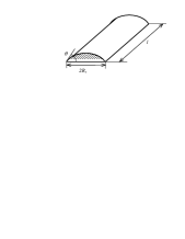
Figure 4: Reference system to describe the 2D drop. The contact angle $\theta$ is shown too.

The volume $V$ of the stripe per its length $l$ does not change with time:

$$V/l={R_{x}^{2}\over 2\,\sin^{2}\theta}\,(\theta-\sin\theta\,\cos\theta),$$ (39)

where $R_{x}$ is the half-width of the stripe, see Fig. 4. The dynamic contact angle $\theta$ can be calculated from Eq. (39), provided that $R_{x}$ is known. It can be shown by the direct calculation of $U^{(0)}$ (35) and the dissipation function $T$ (6) that Eq. (8) with the substitution $q_{j}\rightarrow R_{x}$ reduces to the equation

$$\dot{R_{x}}={\sigma\over\xi}\,(\cos\bar{\theta}_{eq}-\cos\theta)-{1\over 2\,\xi l}\,{{\rm d}\Delta U\over{\rm d}R_{x}}$$ (40)

The first-order correction to the drop energy $\Delta U$ can be calculated from Eq. (36) by following the guidelines of Garoff . Its explicit expression for the chosen geometry is given in Appendix B.

The kinetics of the relaxation is shown in Fig. 5. The relaxation kinetics for the drop on the ideal substrate with the equilibrium value of the contact angle equal to the value of $\bar{\theta}_{eq}$ is also shown for comparison. The half-width of the drop on the ideal substrate relaxes to its equilibrium value $R^{\ast}$ that is related to the volume of the drop through Eq. (39) written for $\theta=\bar{\theta}_{eq}$ and $R_{x}=R^{\ast}$. We chose $R^{\ast}/\lambda=100$ for Fig. 5.

The stick-slip motion is illustrated in the insert in Fig. 5.

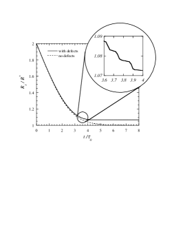
Figure 5: Temporal evolution of the half-width $R_{x}$ of the drop with and with no defects with the same initial ($t=0$) value of $R_{x}=2\,R^{\ast}$ and for $R^{\ast}=100\lambda$ and $\bar{\theta}\approx 55^{\circ}$. The latter value corresponds to the defect radius $r=0.2\lambda$, $\theta_{1}=70^{\circ}$, and $\theta_{2}=50^{\circ}$.

Note that the contact line in its final position for the non-ideal case is pinned in a metastable state so that the final 2D radius of the drop is larger than $R^{\ast}$. The final contact angle (the equilibrium receding contact angle) thus differs from that for an ideal surface. Because the contact line is being stuck on the defects, its motion is slowed down. However, the presence of defects does not change strongly the relaxation time. It remains of the order of $\tau_{0}=R^{\ast}\xi/\sigma$ because this deceleration is compensated by the acceleration during the slip motion.

Fig. 5 shows the impact of the defects on the relaxation. The relaxation time appears to be smaller in the presence of defects than in the ideal case (no defects) because the contact line is pinned by defects whereas it would have continued to move on the ideal surface.

It should be noted that this model is just a first step towards the description of contact line kinetics on a non-ideal substrate. In reality, the different portions of the contact line slip at different moments in time (cascades of slips are observed e. g. in Wong ). This means that the liquid flows in the direction parallel to the contact line to the distances much larger than the defect size, i. e. the first-order approximation is not adequate. The direction of this flow reverses frequently. This effect can lead to the expression like Eq. (31) and to a large relaxation time.

IV Conclusions

This article deals with two important issues concerning contact line dynamics. First, it discusses the local versus non-local approaches to contact line motion. While the local approach consists in postulating a direct relationship between the normal contact line velocity and the dynamic contact angle at a given point of the contact line, the nonlocal approach starts from a more general hypothesis about the form of the dissipation function of the droplet. These approaches give the same results for very small contact angles or for the normal contact line velocity that does not vary along the contact line, which is the case of a drop that has the shape of a spherical cap. In other cases (large contact angle, non-spherical drops) the results of these two approaches differ. We carried out calculations assuming that the drop surface is a spheroid. In reality, its surface is not a spheroid and has a constant curvature. More theoretical work is needed to overcome this approximation.

The second issue treated in this article is the influence of surface defects on contact line dynamics. In the approximation of a 2D drop, it is assumed that the contact line remains straight during its motion. In this approximation, the stick-slip microscopic motion does not influence the average dynamics strongly. The defects manifest themselves by changing the final position of the contact line by pinning it in a metastable state. Therefore, the relaxation is more rapid than that on an ideally clean surface simply because it is terminated earlier.

Appendix A Derivation of the dynamic equations for $r_{x}$ and $r_{y}$

We used the $Mathematica^{\rm TM}$ system for the analytical computations. We find first the dissipation function $T$. The contact line can be described by the equation

$$F(x,y)=0\quad\mbox{with}\quad F(x,y)={\frac{x^{2}}{R_{x}^{2}}}+{\frac{y^{2}}{R_{y}^{2}}}-1,$$ (41)

where $R_{x}$ and $R_{y}$ are time-dependent. By using the well-known formula of differential geometry $v_{n}=-\dot{F}/|\nabla F|$, the integral (6) can be written in an explicit form. In order to obtain the first order approximation for $T$, one can use the expansion (15). We need to keep only the second-order terms. Since the integrand is a quadratic form with respect to $\dot{r_{x}},\dot{r}_{y}$, one can put $r_{x},r_{y}=0$ in it. The resulting expression can be integrated to obtain the explicit expression for the dissipation function

$$T={\xi\,\pi\,R^{3}\,\sin^{3}\theta_{s}\over 8}(3\,\dot{r}_{x}^{2}+3\,\dot{r}_{y}^{2}-2\,\dot{r}_{x}\,\dot{r}_{y}).$$ (42)

It is easy to find out that $T\geq 0$ always holds as it should be.

It is more difficult to obtain the drop interface area

$$A_{VL}=\int\limits_{A_{SL}}\sqrt{1+\left(\frac{\partial z}{\partial x}\right)^{2}+\left(\frac{\partial z}{\partial y}\right)^{2}}\;{\rm d}A,$$ (43)

where the function $z=z(x,y)$ is defined by Eq. (11). After the integration over $y$, Eq. (43) reduces to

$$A_{VL}=4\,b\int\limits_{0}^{R_{x}}\arctan\left(\frac{b}{d}\sqrt{1-\frac{d^{2}}{b^{2}}-\frac{x^{2}}{a^{2}}}\right)\,\sqrt{1-\frac{x^{2}}{a^{2}}\,\epsilon}\;{\rm d}x,$$ (44)

where $\varepsilon=1-R_{y}^{2}/R_{x}^{2}\sim(r_{x}-r_{y})\ll 1$. The subsequent development of the integrand into the series over $\epsilon$ and its integration term-by-term results in

$$A_{VL}=a\,\pi\,\left[2\,\left(b-d\right)-\frac{\epsilon}{6\,b^{2}}\left(2\,b^{3}-3\,b^{2}\,d+d^{3}\right)-\right.$$

$$\left.\frac{\epsilon^{2}}{160\,b^{4}}\left(8\,b^{5}-15\,b^{4}\,d+10\,b^{2}\,d^{3}-3\,d^{5}\right)\,\right].$$ (45)

This expression can be developed into a series with respect to $r_{x},r_{y}$ by using Eqs. (12, 13-15). Its substitution into Eq. (9) leads to the explicit expression for $U$:

$$U=\sigma\pi R^{2}\Bigl{\{}2-3\,\cos\theta_{s}+\cos^{3}\theta_{s}+$$

$${\sin^{2}\theta_{s}\over 8}\left[A\left(r_{x}^{2}+r_{y}^{2}\right)-2B\,r_{x}\,r_{y}\right]\Bigr{\}},$$ (46)

where

$$\begin{array}[]{c}A=\left[(288+491\,\cos\theta_{s}+374\,\cos^{2}\theta_{s}+107\,\cos^{3}\theta_{s})\cdot\right.\\ \left.(1-\cos\theta_{s})\right]/[45(1+\cos\theta_{s})],\\ B=\left[(72+409\,\cos\theta_{s}+346\,\cos^{2}\theta_{s}+73\,\cos^{3}\theta_{s})\cdot\right.\\ \left.(1-\cos\theta_{s})\right]/[45(1+\cos\theta_{s})].\end{array}$$ (47)

It is easy to show that the expression in the square brackets in Eq. (46) is positive for an arbitrary $\theta_{s}$. It means that the function $U(r_{x},\,r_{y})$ has its minimum at the point $(r_{x}=0,\,r_{y}=0)$, i.e. for the drop that has the shape of the spherical cap. This result was expected.

The substitution of Eqs. (46, 42) into Eq. (8) written for $q_{j}=(r_{x},r_{y})$ results in the set of Eqs. (18) and thus concludes their derivation.

Appendix B Expression for the first order correction to the drop energy caused by defects

The accepted assumptions facilitate calculation of the $\Delta U(R_{x})$. The resulting function is periodical with the period $\lambda/2$, so that for $r<\lambda/4$ it can be presented in the form

$${\frac{\Delta U}{2\,\sigma\,\rho\,\Delta c}}=-\left\{\begin{array}[]{rl}\varepsilon^{2}\rho-\left[r^{2}\arcsin(\rho/r)+\right.\\ \left.\rho(r^{2}-\rho^{2})^{1/2}\right]/\lambda,&0\leq\rho<r\\ \varepsilon^{2}\left(\rho-\lambda/4\right),&r\leq\rho<{\frac{\lambda}{2}}-r\\ \varepsilon^{2}\left(\rho-\lambda/2\right)+\\ \Bigl{\{}r^{2}\arcsin\left[\left(\lambda/2-\right.\right.\\ \left.\left.\rho\right)/r\right]+\left(\lambda/2-\rho\right)\Bigl{[}r^{2}-\\ \left(\lambda/2-\rho\right)^{2}\Bigr{]}^{1/2}\Bigr{\}}/\lambda,&{\frac{\lambda}{2}}-r\leq\rho<{\frac{\lambda}{2}}\end{array}\right.$$ (48)

where $\rho$ is the fractional part of $2R_{x}/\lambda$, multiplied by $\lambda/2$, and $\Delta c=\cos\theta_{2}-\cos\theta_{1}$. Since $R_{x}\gg\lambda$, the presence of defects generates many local minima of the function $U(R_{x})$ near its global minimum. These minima represent the metastable states. According to this model, the contact line is pinned in the minimum closest to its initial position.

References

- (1) C. Huh and L. E. Scriven, J. Colloid Interf. Sci. 35, 85 (1971).
- (2) E. B. Dussan V. and S. H. Davis, J. Fluid Mech. 65 part 1, 71 (1974).
- (3) The hydrodynamic flow calculations (see e.g. Huh ; Sh ; Sepp ), which use other contact line motion models show that they are all compatible with these experiments.
- (4) L. Mahadevan and Y. Pomeau, Phys. Fluids 327, 155 (1999).
- (5) P.-G. de Gennes, Rev. Mod. Phys. 57, 827 (1985).
- (6) C. Andrieu, D. A. Beysens, V. S. Nikolayev, and Y.Pomeau, J. Fluid Mech. 453, 427 (2002).
- (7) Y. D. Shikhmurzaev, Phys. Fluids 9, 266 (1997).
- (8) P. Seppecher, Int. J. Eng. Sci. 34, 977 (1996).
- (9) Y. Pomeau, Comptes Rendus Acad. Sci., Serie IIb 328, 411 (2000).
- (10) R. G. Cox, J. Fluid Mech. 168, 169 (1986).
- (11) O. V. Voinov, Fluid Dynamics 11, 714 (1976).
- (12) T. D. Blake and J. M. Haynes, J. Colloid Interface Sci. 30, 421 (1969).
- (13) E. B. Dussan V., J. Fluid Mech. 174, 381 (1987).
- (14) M.J. de Ruijter, J. De Coninck, and G. Oshanin, Langmuir 15, 2209 (1999).
- (15) L. D. Landau and E. M. Lifschitz, Mecanique, 3rd ed. (Mir, Moscou, 1969).
- (16) A. Hazareesing and M. Mézard, Phys. Rev. E 60, 1269 (1999).
- (17) L. W. Schwartz and S. Garoff, Langmuir 1, 219 (1985).
- (18) P. Collet, J. De Coninck, F. Dunlop, and A. Regnard, Phys. Rev. Lett. 79, 3704 (1997).
- (19) E. Schäffer and P.-Z. Wong, Phys. Rev. Lett. 80, 3069 (1998).