Quasi-static relaxation of arbitrarily shaped sessile drops

Abstract

We study a spontaneous relaxation dynamics of arbitrarily shaped liquid drops on solid surfaces in the partial wetting regime. It is assumed that the energy dissipated near the contact line is much larger than that in the bulk of the fluid. We have shown rigorously in the case of quasi-static relaxation using the standard mechanical description of dissipative system dynamics that the introduction of a dissipation term proportional to the contact line length leads to the well known local relation between the contact line velocity and the dynamic contact angle at every point of an arbitrary contact line shape. A numerical code is developed for 3D drops to study the dependence of the relaxation dynamics on the initial drop shape. The available asymptotic solutions are tested against the obtained numerical data. We show how the relaxation at a given point of the contact line is influenced by the dynamics of the whole drop which is a manifestation of the non-local character of the contact line relaxation.

I Introduction

The spreading of a liquid drop deposited on a solid substrate has many technological applications stimulating active research on acquiring accurate knowledge on its relaxation that follows the deposition. More specifically, one is interested to know how the relaxation rate depends on the initial drop shape and the properties of the contacting media. It is a complex theoretical problem and there are numerous studies devoted to drop relaxation using different approaches and techniques: e.g. macroscopic Huh and Scriven (1971); Voinov (1976); Dussan (1979); Tanner (1979); de Gennes (1985); Huh and Mason (1977); Cox (1986) and more recent microscopic approaches using molecular dynamic simulations Blake et al. (1997),de Ruijter et al. (1999a) and Monte-Carlo simulations of 3D lattice gas Tan (1999) and 2D Cheng and Ebner (1993) and 3D Ising model Pesheva and de Coninck (2004) etc., to mention just few of them.

In the case of partial wetting this problem turns out to be very difficult because of the presence of the triple gas-liquid-solid contact line. Since the work Huh and Scriven (1971), it has become obvious that the contact line motion cannot be described with the classical viscous hydrodynamics approach that uses the no-slip boundary condition at the solid surface. The velocity ambiguity at the moving contact line leads to the un-physical divergences of the hydrodynamic pressure and viscous dissipation. Multiple approaches were suggested to overcome this problem. Among the most popular solutions one can name a geometrical cut-off de Gennes (1985) or the local introduction of the slip near the contact line Huh and Mason (1977). One finds experimentally Andrieu et al. (2002); Narhe et al. (2004) that while the dissipation is finite, it is very large with respect to the bulk viscous dissipation. Several physical mechanisms are suggested to describe the contact line motion Blake and Haynes (1969); Shikhmurzaev (1997).

Following a suggestion in de Gennes (1985), a combined approach was proposed in de Ruijter et al. (1999b) considering both, the bulk viscous dissipation and the dissipation occurring at the moving contact line, to study the drop relaxation in the partial wetting regime. A phenomenological dissipation per unit contact line length was introduced. It was taken to be proportional to the square of the contact line velocity $v_{n}$ (the first term symmetric in $v_{n}$) in the direction normal to the contact line. There the standard mechanical description of dissipative system dynamics was applied to describe the time evolution of the drop contact line in the case of a spherical cap approximation for the drop shape in the quasi-static regime. Considering the drop as a purely mechanical system, the driving force for the drop spreading was balanced by the rate of total dissipation. No assumption was made for a particular line motion mechanism.

This approach was further generalized to any contact line shape in Nikolayev and Beysens (2002) by writing the energy dissipated in the system per unit time as

$$T=\oint{\xi v_{n}^{2}\over 2}\,dl\ ,$$ (1)

where the integration is over the contact line of the drop and $\xi$ is the dissipation coefficient.

In the present work we employ this approach to study the quasi-static relaxation of arbitrarily shaped drops in the partial wetting regime. It is assumed here that the energy dissipated near the contact line is much larger than that in the bulk of the fluid. In Section II we show that this approach actually leads to the local relation (first obtained in the molecular-kinetic model of contact line motion of Blake and Haynes Blake and Haynes (1969)) between the contact line velocity and the dynamic contact angle at every point of an arbitrarily shaped contact line. In Section III we describe a numerical 3D code for studying the relaxation of an arbitrarily shaped drops starting directly from the variational principle of Hamilton, taking into account the friction dissipation during the contact line motion. In Section IV we obtain numerically and discuss the quasi-static relaxation of a drop with different initial shapes. Section V deals with our conclusions.

II THE MODEL

We consider a model system consisting of a 3D liquid drop placed on a horizontal, flat and chemically homogeneous solid substrate. Both the drop and the substrate are surrounded by an ambient gas and it is assumed that the liquid and the gas are mutually immiscible. Initially the drop deposited on the substrate is out of equilibrium. Under the action of the surface tension, the incompressible liquid drop relaxes towards spherical cap shape. The drop is assumed to be small enough so that the influence of the gravitation on its shape can be neglected. According to the capillary theory Finn (1986); Landau and Lifshitz (1987), the potential energy of the system is:

$$U=A_{lg}\sigma_{lg}+A_{ls}\sigma_{ls}+A_{sg}\sigma_{sg},$$ (2)

where the surfaces $A_{lg}$, $A_{ls}$, and $A_{sg}$ (with corresponding surface tensions $\sigma_{lg}$, $\sigma_{ls}$, and $\sigma_{sg}$) separate the liquid/gas, liquid/solid, and solid/gas phases respectively. In accordance with the approach described in de Ruijter et al. (1999b); Blake and Haynes (1969); Nikolayev and Beysens (2002), we assume that with the moving contact line a dissipation function $T$ is related, given by Eq.(1).

According to the variational principle of Hamilton one writes:

$$\int_{t_{0}}^{t_{1}}(\delta K+\delta W)\,dt\ =0,$$ (3)

where $\delta W$ is the virtual work of the active forces and $\delta K$ is the variation of the kinetic energy of the system. The virtual work is $\delta W=-\delta U+\delta W_{1}$, where $\delta W_{1}$ is the virtual work related to the friction dissipation Eq. (1). A class of virtual displacements is considered in Eq. (3) satisfying the conditions of immiscibility, of conservation of the area of the solid surface and the condition of constant volume $V$. Since the Lagrangian is ${\mathcal{L}}=K-U$, the variational condition given by Eq. (3) can be put in the following form:

$$\int_{t_{0}}^{t_{1}}(\delta{\mathcal{L}}+\delta W_{1})\,dt\ =0.$$ (4)

The contribution of the kinetic energy of the fluid motion is assumed to be negligible because we consider a quasi-static relaxation here, so that $\mathcal{L}=-U$.

The radius-vectors $\vec{R}$ of the points of the liquid/gas interface $A_{lg}$ are taken as generalized coordinates. These coordinates are not independent, their displacements have to satisfy the condition of constant drop volume. Taking into account this condition by introducing a Lagrange multiplier $\lambda$ and adding the term $\lambda V$ into Eq. (4) one obtains:

$$\int_{t_{0}}^{t_{1}}(-\delta U+\delta W_{1}+\lambda\delta V)\,dt\ =0.$$ (5)

The Lagrange multiplier $\lambda$ (its physical meaning is the pressure jump across the drop surface $A_{lg}$) varies in time. So in the quasi-static regime one has the following equation

$$-\delta U+\delta W_{1}+\lambda\delta V\ =0,$$ (6)

where $\delta W_{1}$ is given by (see, e.g., Landau and Lifshitz (2003))

$$\delta W_{1}=-\xi\oint_{L}v_{n}\delta{\vec{R}}\,dl\,.$$ (7)

The variation of the potential energy under the constant volume constraint reads Finn (1986)

$$\delta(-{U}+\lambda V)=\int_{A_{lg}}(2\sigma_{lg}k-\lambda)\delta{\vec{R}}\,dA_{lg}+\sigma_{lg}\oint_{L}(\cos\theta_{eq}-\cos\theta)\delta{\vec{R}}\,dl,$$ (8)

where $k$ is the mean curvature of the liquid/gas interface $A_{lg}$; $\delta\vec{R}$ is the virtual displacement of the points normal to the drop surface $A_{lg}$ in the first and to the contact line $L$ in the second integrals respectively; $\theta$ is the dynamic contact angle, $\theta_{eq}$ is the equilibrium contact angle defined by the well known Young equation:

$$\cos\theta_{eq}=(\sigma_{gs}-\sigma_{ls})/\sigma_{lg}.$$ (9)

Substituting Eqs. (7) and (8) in Eq. (6) and taking into account the independence of the virtual displacements of the points of the interface $A_{lg}$ and of the contact line $L$ (due to which each of the integrands must be equated to zero separately), one obtains the Laplace equation

$$-2\sigma_{lg}k+\lambda=0,$$ (10)

from which the surface shape can be obtained at any time moment and the equation

$$(\cos\theta_{eq}-\cos\theta({\vec{R}}))={\xi\over\sigma_{lg}}{\vec{v}}_{n}({\vec{R}})\,,\ {\vec{R}}\in L\$$ (11)

valid at the contact line. Eq. (11) serves as a boundary condition for Eq. (10). For a given volume $V$ and arbitrary initial contact line position $L_{0}$, Eqs. (10,11) define the evolution of the drop shape and of the drop contact line. However, in our calculations we will not use Eqs. (10,11) directly, we will use Eqs. (6, 7) instead.

The final drop shape is that of a spherical cap. The radius $R^{*}$ of its contact line serves as a characteristic length scale. The time

$$\tau_{0}=R^{*}\xi/\sigma_{lg}$$ (12)

defines a characteristic time scale.

When the spherical cap approximation can be used for the drop shape then at any moment of time only one parameter is needed to specify the instantaneous configuration of the drop: either the time-dependent base radius $R(t)$ or the dynamic contact angle $\theta(t)$. The drop volume conservation condition implies a relationship between $R(t)$ and $\theta(t)$:

$$R^{3}(t)=\frac{3V}{\pi}\frac{[1+\cos\theta(t)]\sin\theta(t)}{[1-\cos\theta(t)][2+\cos\theta(t)]}\ .$$ (13)

Thus Eq. (11) leads to the following ordinary differential equation for the dynamic contact angle $\theta(t)$ de Ruijter et al. (2000):

$$\frac{d\theta}{dt}=\left(\frac{\pi}{3V}\right)^{1/3}\left\{[1-\cos\theta(t)][2+\cos\theta(t)]^{2}\right\}^{2/3}[\cos\theta(t)-\cos\theta_{eq}]\ .$$ (14)

Note, that the well known dependencies, $\theta\left(t\right)\sim t^{-3/7}$ and $R\left(t\right)\sim t^{1/7}$, (see, e.g., de Ruijter et al. (1999b); de Ruijter et al. (2000); Rieutord et al. (2002)) are asymptotic solutions of Eqs. (13, 14) for small contact angles.

Nikolayev and Beysens Nikolayev and Beysens (2002) considered the relaxation of an elongated drop by assuming its surface to be a part of a spheroid at any time moment. The contact line is then ellipse with half-axes $R^{*}(1-r_{x})$ and $R^{*}(1+r_{y})$ where the relative deviations $r_{x}$ and $r_{y}$ were assumed to be small, $0<r_{x},r_{y}<<1$. Such an approximation can be adequate at the end of the relaxation. However, it allowed only the case $\theta_{eq}<\pi/2$ to be considered. Nikolayev and Beysens obtained exponential asymptotic solutions for $r_{x}(t)$ and $r_{y}(t)$. Two relaxation times were identified. One of them appears when the drop surface is a spherical cap, i.e., when $r_{x}(0)=-r_{y}^{(}0)$:

$$\tau_{s}=\tau_{0}/\left[\sin^{2}\theta_{eq}\left(2+\cos\theta_{eq}\right)\right].$$ (15)

When the initial contact line is an ellipse with $r_{x}(0)=r_{y}(0)$, the relaxation time obtained using spheroidal approximation reads

$$\tau_{n}=45\tau_{0}\left(1+\cos\theta_{eq}\right)/\left[\left(108+41\cos\theta_{eq}+14\cos^{2}\theta_{eq}+17\cos^{3}\theta_{eq}\right)\left(1-\cos\theta_{eq}\right)\right].$$ (16)

III Description of the numerical algorithm

The following numerical algorithm was implemented. First, for a given position of the contact line and fixed volume $V$ the equilibrium drop shape is determined. Then the normal projection of the velocity at every point of the contact line is obtained by the help of Eqs. (6, 7). Next, from the kinematics condition

$${{d\vec{R}}\over{dt}}=\vec{v}_{n},$$ (17)

the contact line position at the next instant of time is found explicitly. The above algorithm is repeated for the successive time steps.

The main ingredients of this algorithm are the determination of the equilibrium drop shape with given volume and given contact line, and the calculation of the velocity of the contact line. The drop shape algorithm is essentially an iterative minimization procedure based on the local variations method Chernousko (1965). Here, only a very concise description will be given; more details can be found in Iliev (1995). The drop shape is approximated by a set of flat triangles with total of $N=12781$ vertex points, $N_{L}=360$ of these are located at the contact line (see Fig. 4). For a given contact line, the area of the drop surface is expressed in terms of the coordinates of the $N$ points. The change of the drop shape is achieved by approximation of the virtual displacements. In the $3N-3N_{L}$ coordinate space, the set of all possible displacements of $N-N_{L}$ points is considered while keeping the volume and the contact line constant. We use the Monte Carlo scheme for choosing the points which we will try to move. At every iteration step the drop shape is changed in such a way that the free energy decreases while the drop volume is kept constant. Thus eventually the minimal drop surface is found.

The approximation of the normal projection of the velocity of the contact line at each of the $N_{L}=360$ vertex points of the contact line is obtained by solving the finite approximation of Eq. (6). The method takes into account that the finite approximation of Eq. (6) is described by energy and volume variations under displacements of these points. The correctness of the obtained solution at every time step is checked by keeping track of the accuracy with which the coordinates of the points from the surface satisfy the Laplace condition and Eq. (11). For given contact line and volume, the initial approximation of the drop shape is found in the following way. First, for the given volume we find the spherical cap approximation. Then we perform an iterative procedure which transforms the contact line gradually while the volume is kept fixed until the desired contact line is obtained.

In order to ensure better work of the minimization procedure, we perform regular check of the surface mesh and re-adjust the mesh to keep the approximation of the liquid/gas interface uniform. This allows us to maintain high accuracy in determining the contact angle with an error of the order of $0.01^{\circ}$. At a given contact line node point the contact angle is defined as the angle between the plane of the substrate and the plane of the triangle whose corner coincides with that point.

IV Results and Discussion

IV.1 Spherical cap relaxation

To test the described above 3D code, we check it against the numerical solution of Eqs. (13,14) obtained for a broad interval of values of the equilibrium contact angle $\theta_{eq}$. The initial contact line radius differs from its equilibrium (final) value $R^{*}$, the deviation being $\Delta R_{0}=R(0)-R^{*}$. As follows from Eq. (12), we can set $R^{*}=1$ and $\tau_{0}=1$ without a loss of generality.

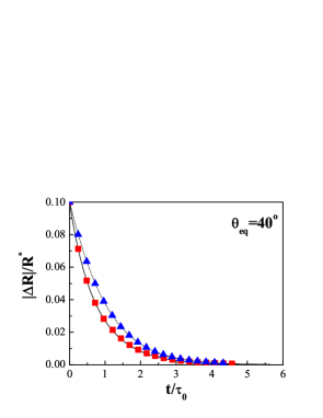
Figure 1: (Color online) Time dependence in $\tau_{0}$ units of the absolute value of the deviation of the contact line radius from the equilibrium value $|\Delta R(t)|$ in $R^{*}$ units for $\theta_{eq}=40^{\circ}$ calculated for a drop with a spherical cap shape. Solid and dashed lines: solutions of Eqs. (14), (13) for $R(0)<R^{*}$ and $R(0)>R^{*}$ respectively. Squares and triangles: numerical 3D calculations for $R(0)<R^{*}$ and $R(0)>R^{*}$ respectively (for convenience, every $20^{\textrm{th}}$ data point is displayed).

A comparison of the numerical data, obtained by both methods and displayed in Fig. 1, shows a very high (less than 1%) accuracy of the 3D code. It can be seen from Fig. 1 that for the same values of $\theta_{eq}$ and $|\Delta R_{0}|$ the solutions for receding contact line, $R(0)>R^{*}$, and advancing contact line, $R(0)<R^{*}$, differ. This follows directly from Eqs. (11) and (13) since the following inequality holds

$$|\cos\theta(R^{*})-\cos(\theta(R^{*})+\delta\theta)|\neq|\cos\theta(R^{*})-\cos(\theta(R^{*})-\delta\theta)|$$ (18)

By substituting this inequality in Eq. (11) it follows that for the same absolute value of the deviation $|\Delta R_{0}|$ there is a difference in the initial velocities for advancing and receding contact lines.

We studied the possibility to fit the obtained numerical solutions for $R(t)$ by power and exponential functions. We use the following definition of the relative error of the fit $\overline{R(t)}$ with respect to $R(t)$:

$$\Delta=\max^{t^{*}}_{t=0}\left(\frac{\left|R\left(t\right)-\overline{R\left(t\right)}\right|}{\left|R\left(t\right)-R^{*}\right|}\right)$$ (19)

For small initial deviations $|\Delta R_{0}|$, it turns out that the exponential fit with

$$\overline{R\left(t\right)}=R^{*}+|\Delta R_{0}|\exp(-t/\tau)\ ,$$ (20)

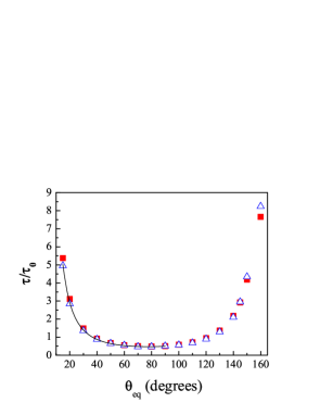
Figure 2: (Color online) The spherical cap relaxation time $\tau$ in $\tau_{0}$ units as function of the equilibrium contact angle $\theta_{eq}$ for initial deviation $|\Delta R_{0}|=0.03$ in $R^{*}$ units: the solid squares are the results for $\Delta R_{0}=0.03$; the empty triangles are the results for $\Delta R_{0}=-0.03$ and the solid line is $\tau_{s}$ (Eq. (15)) for $\theta_{eq}<90^{\circ}$.

where $\tau$ is the only fitting parameter, describes very well the data for all studied values of $\theta_{eq}$. The relaxation time $\tau$ depends on the initial deviation $\Delta R_{0}$ and when $|\Delta R_{0}|\to 0$, $\tau$ tends to the spherical relaxation time $\tau_{s}$ (Eq. 15).

We first obtained the solutions for $|\Delta R(t)|$ by the 3D numerical simulation for initial deviation $|\Delta R_{0}|=0.03$ and for contact angles $15^{\circ}\leq\theta_{eq}\leq 165^{\circ}$. By fitting the obtained solutions with exponential decay function we determined the corresponding relaxation times $\tau$ as function of the equilibrium contact angle $\theta_{eq}$ in the above interval of values. This dependence is shown in Fig. 2: the squares are the results for $\Delta R_{0}=-0.03$ and the open triangles are for $\Delta R_{0}=0.03$. The thin solid line in the figure is the spherical relaxation time $\tau_{s}$ (see Eq. (15)) in the interval $\theta_{eq}<90^{\circ}$. The exponential approximations of the solutions are obtained in the time interval $[0,t_{end}^{100}]$ determined so that $\left|R\left(t_{end}^{100}\right)-R^{*}\right|=0.01\left|R\left(0\right)-R^{*}\right|$, that is the amplitude of the initial deviation has decreased hundred times. The exponential approximation is obtained under the condition that it coincides with the numerical solution at the initial and final points, $\{0,t_{end}^{100}\}$. The maximal relative deviation of the obtained exponential approximations from the numerical solutions does not exceed $\Delta<3\%$. When $|\Delta R_{0}|$ decreases the precision of the exponential approximation increases. When $|\Delta R_{0}|$ increases, e.g. $|\Delta R_{0}|=0.1,0.2$, the precision of the exponential approximation to the numerical solution of Eqs. (14, 13) in the time interval $\left[0,t_{end}^{100}\right]$ decreases.

When the equilibrium contact angle $\theta_{eq}$ increases the relative deviation $\Delta$ decreases. The cases of advancing and receding contact lines differ with less than $1-2\%$ for $\theta_{eq}\geq 40^{\circ}$. Also when $|\Delta R_{0}|$ increases, so does the deviation of the relaxation exponent $\tau$ (Eq. 20) from the spherical relaxation time $\tau_{s}$. When the exponential approximation in the interval $\left[0,t_{end}^{100}\right]$ becomes unacceptable, e.g., when $\Delta$ more than $3\%$, or $-\frac{1}{3}R^{*}\leq\Delta R\leq 3R^{*}$ then a good approximation could be obtained either by splitting the interval $\left[0,t_{end}^{100}\right]$ into several subintervals and approximating the numerical solution on every such subinterval with an exponential function with a specific relaxation time $\tau$ or by fitting the numerical solution with a second or higher order exponential decay function. For example, for the considered cases $|\Delta R_{0}|=0.1,0.2$ the fit with an exponential decay function of the second order

$$\overline{R\left(t\right)}=R^{*}+a_{1}\exp(-t/\tau_{1})+a_{2}\exp(-t/\tau_{2})\ ;|a_{1}|\geq|a_{2}|\ ,$$ (21)

where $a_{1},\tau_{1},a_{2},\tau_{2}$ are the fitting parameters, on the interval $\left[0,t_{end}^{100}\right]$ becomes much better than with the first order exponential decay function (Eq. (20)) especially for $\theta_{eq}<40^{\circ}$. For example for $\theta_{eq}=40\raisebox{4.30554pt}{\scriptsize o}$ and $\Delta R_{0}=-0.1$ the maximal deviation with Eq. (21) is less than $1\%$ as compared to $10\%$ with Eq. (20).

	$\tau_{s}/\tau_{0}$	$a_{1}$	$\tau_{1}/\tau_{0}$	$a_{2}$	$\tau_{2}/\tau_{0}$	$\Delta$
$\theta_{eq}=10^{\circ}$	$11.1$	$-0.08$	10.8	$-0.02$	3.9	2.7%
$\theta_{eq}=40^{\circ}$	$0.87$	$-0.084$	0.866	$-0.016$	0.35	1%
$\,\theta_{eq}=70^{\circ}$	$0.48$	-0.092	0.484	-0.008	0.248	0.08%

Table 1: Relative deviation $\Delta$ of the exponential approximation of second order

As can be seen from Table 1 , $\tau_{1}$ is close to $\tau_{s}$ and the amplitude $a_{2}$ is sufficiently large so that the influence of the second exponent should not be neglected. When the equilibrium contact angle $\theta_{eq}\to\pi/2$ the second amplitude $a_{2}$ decreases. For contact angles $\theta_{eq}\in(0,\pi/2]$ the amplitude $a_{2}$ in the case $\Delta R_{0}=0.1$ is smaller than in the case $\Delta R_{0}=-0.1$. For contact angles $\theta_{eq}>\pi/2$ the opposite is true.

For small contact angles, e.g., $\theta_{eq}=3^{\circ},5^{\circ}$ we tried to fit our data also with a power function $f\sim t^{1/7}$. It appears that it is possible to find a time interval at the beginning where the numerical data is well described by the power function but the overall behavior is still better described by the exponential approximation.

IV.2 Relaxation of elongated drops

Here we consider the relaxation of a liquid drop when the initially elliptical contact line (with initial deviations $r_{x}(0)=r_{y}(0)=|\Delta R_{0}|>0$) relaxes towards circular contact line. We study the time relaxation $r_{x}(t)$ and $r_{y}(t)$ of the two extreme points $M$ and $N$ of the ellipse, where $R^{*}(1-r_{x})$ and $R^{*}(1+r_{y})$ are the half-axes of the contact line ellipse. The goal is to check the validity of the spheroidal approximation in Nikolayev and Beysens (2002) and extend the results to the domain $\theta>90^{\circ}$. The analysis of the data obtained by the method described in Section 3 shows that the time relaxation for initial deviations up to $r_{x}(0)=0.2$ is again well described by an exponential decay function of the first or second order (i.e. by the sum of two exponential functions with different relaxation times) in the time interval $[0,t_{end}^{100}]$. The error of the fit is $\Delta<3\%$. The obtained values for the relaxation time $\tau$ (Eq. (20)) for contact angles in the interval $15^{\circ}\leq\theta\leq 165^{\circ}$, $r_{x}(0)=0.03$, are shown in Fig. 3. For $15^{\circ}\leq\theta_{eq}\leq 50^{\circ}$ the relative deviation from Eq. (16)

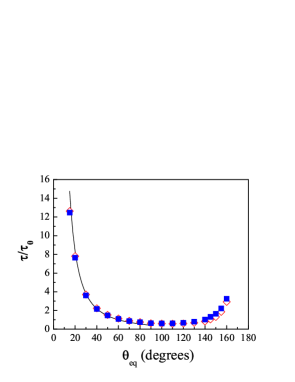
Figure 3: (Color online) The relaxation time for the elongated drop in $\tau_{0}$ units as a function of the equilibrium contact angle $\theta_{eq}$ for $r_{y}(0)=r_{x}(0)=0.03$ in $R^{*}$ units: the solid squares and empty diamonds are the results for the exponential fits of $r_{x}(t)$ and $r_{y}(t)$ respectively. The solid line is $\tau_{n}$ (Eq. (16)) for $\theta_{eq}<90^{\circ}$.

is of the order of $2-4\%$. Outside of this interval it increases fast and for $\theta_{eq}\sim 90^{\circ}$ it reaches $\sim 60\%$. The increase of the deviation is due to the fact that the approximation of the spheroidal cap to the quasi-stationary drop shape is worsening with the increase of the contact angle $\theta_{eq}$. Note that while the surface curvature $k$ has to remain constant along the surface according to Eq. 10, it varies as much as 20% for the spheroid with $r_{x}(0)=0.1$. In the 3D simulation, the curvature variation along the surface is less than 0.5% which is a good accuracy.

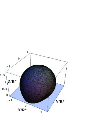
Figure 4: (Color online) The initial drop shape with elliptical contact line and minimal surface for $\theta_{eq}=120^{\circ}$, $r_{x}(0)=0.2$ in $R^{*}$ units and volume $V/{R^{*}}^{3}=5.44$.

The numerical results for $\theta_{eq}=120^{\circ}$ and $r_{x}(0)=0.2$, are shown in Figs. 4-7. The results for other contact angles look qualitatively the same way. The initial drop shape is shown in Fig. 4. The volume of the drop is chosen so that the final shape is the spherical cap with the radius of the contact line $R^{*}=1$ and a contact angle $\theta_{eq}=120^{\circ}$. The contact line evolution is shown in Fig. 5. The time evolution of the contact angle along the contact line is shown in Fig. 6.

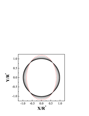
Figure 5: (Color online) The contact line positions obtained with time step $(0.2\tau_{0})$ for $\theta_{eq}=120^{\circ}$ and $r_{x}(0)=0.2$ in $R^{*}$ units. The dashed line is the initial position.

Figure 6: The contact angle as a function of the polar angle $\varphi$ at successive moments of time $\left\{0,0.2n,n=1,2,...\right\}$ in $\tau_{0}$ units for $\theta_{eq}=120^{\circ}$ and $r_{x}(0)=0.2$.

The algorithm efficiency can be checked against Eq. (11) which was not directly used. Fig. 6 shows how good the algorithm precision is: the difference between the slopes of the two straight lines is less than $2\%$.

Note that for equal initial deviations $r_{x}(0)=r_{y}(0)$ at $M$ and $N$ the initial contact angles and the initial velocities at both points are different. From the fact that the relaxation times for both $r_{x}$ and $r_{y}$ are close (when exponential approximation Eq. (20) is used) it does not follow that the velocities of both points are close as it would seem if one simply differentiates Eq. (20) with respect to time $t$. This can be seen if one examines carefully Figs. 6 and 7.

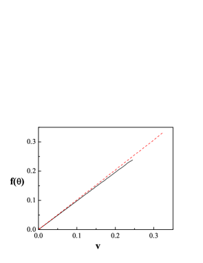
Figure 7: (Color online) The dependence of the function $f(\theta)=|\cos\theta(t)-\cos\theta_{eq}|$ on the contact line velocity in two contact line points for $\theta_{eq}=120^{\circ}$ and $r_{x}(0)=0.2$ in $R^{*}$ units. The solid line corresponds to $v=dr_{y}/dt$, and dashed line to $v=dr_{x}/dt$ (in $R^{*}/\tau_{0}$ units).

When the initial deviations are in the interval $(-\frac{1}{3}R^{*},3R^{*})$ then a good approximation could be obtained either by splitting the time interval into several subintervals and approximating the numerical solution on every such subinterval with an exponential function with a specific relaxation time $\tau$ or by fitting the numerical solution with a sum of two or more exponential functions.

IV.3 Drops of complicated shapes

We study here the relaxation of drops with some example contact lines to demonstrate how the relaxation at one point of the contact line is influenced by the dynamics of the whole contact line. Consider the relaxation of a drop which is almost a spherical cap except for a local perturbation around one point of the contact line. More specifically, let us consider the relaxation of a drop with a final equilibrium contact angle $\theta_{eq}=50^{\circ}$ and with the initial contact line shown in Fig. 8.

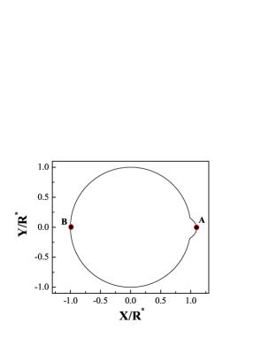
Figure 8: (Color online) The contact line of a drop which is almost a spherical cap with a small deformation around one point.

We find that the time relaxation of the point A$(1.1,0)$ is well approximated by an exponential decay function (21) of the second order: $a_{1}=0.066$, $\tau_{1}=0.163$, $a_{2}=0.024$, $\tau_{2}=0.88$ and the relaxation of the point B$(-1,0)$ by the exponential decay function (20) of the first order with $\tau=1.05$. All the three relaxation times $\{0.163,0.88,1.05\}$ differ from each other and from the relaxation times for spherical and elongated drops $\tau_{s}=0.65$, $\tau_{n}=1.43$ found for $\theta_{eq}=50^{\circ}$ from Eqs. (15,16). It appears thus that the relaxation of the point B is influenced by the perturbation around the point A. Moreover even the type of the relaxation of the point B, whose neighborhood is a part of circle, is not universal and depends on the deformation around the point A. For example when the contact line is of the type shown in Fig. 9 we obtain that the relaxation of the point B is as shown in Fig. 10. It is possible even to find a deformation around A such that the relaxation of the point B is practically linear in a broad time interval.

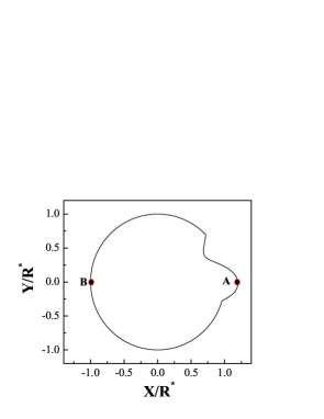
Figure 9: (Color online) The contact line of a drop which is almost a spherical cap with larger deformation around the point A.

Figure 10: Time dependence in $\tau_{0}$ units of $\Delta R(t)$ in $R^{*}$ units at the point B for a drop with initial contact line shown in Fig. 9.

V Conclusions

We have described a method and applied it to simulate the quasi-static relaxation of drops with different initial 3D shapes starting directly from the variational principle of Hamilton, taking into account only the large dissipation in the vicinity of the contact line during the contact line motion.

We have shown rigorously for arbitrary contact line shape using the standard mechanical description of dissipative system dynamics that the introduction of a friction dissipation term proportional to the contact line length in the case of quasi-static relaxation leads to the well known local relation between the contact line velocity and the dynamic contact angle.

We find in the case of spherical cap approximation that the time relaxation of the contact line radius is very well described by an exponential decay function of the first or the second order depending on the magnitude of the initial deviation. The relaxation time $\tau$ depends on the initial deviation $\Delta R_{0}$ and when $|\Delta R_{0}|\to 0$, $\tau$ tends to the spherical relaxation time $\tau_{s}$ defined in Ref. Nikolayev and Beysens (2002). For higher values of $|\Delta R_{0}|$, e.g. $|\Delta R_{0}|=0.1,0.2$, the data is better described by the sum of two exponentials with different relaxation times. The power function fits do not describe well the data.

In the case of elongated drops, the relaxation is again very well described by an exponential decay function. The relaxation time is within 2-4% from that obtained with the spheroid approximation for the drop shape Nikolayev and Beysens (2002) in the range $15^{\circ}\leq\theta_{eq}\leq 50^{\circ}$. For the larger angles, the relaxation time can only be obtained by the described 3D numerical simulation.

Previously exponential relaxation is found in some experimental studies, e.g., in Newman (1968) and more recently in Andrieu et al. (2002). Theoretically, exponential relaxation is found in Nikolayev and Beysens (2002) and asymptotically at long times in de Ruijter et al. (1999b), as well as in the Monte Carlo simulations of the Ising model for drop spreading Pesheva and de Coninck (2004).

By simulating the relaxation of drops of complicated 3D shape, we showed that, although the local Eq. (11) is satisfied, the relaxation at a given point of the contact line is influenced by the relaxation dynamics of the whole drop surface. This is a manifestation of the non-local character of the contact line motion.

References

- Huh and Scriven (1971) C. Huh and L. E. Scriven, J. Colloid Interf. Sci. 35, 85 (1971).
- Voinov (1976) O. V. Voinov, Fluid Dynamics 11, 714 (1976).
- Dussan (1979) E. B. V. Dussan, Ann. Rev. Fluid Mech. 11, 371 (1979).
- Tanner (1979) L. H. Tanner, J. Phys. D: Appl. Phys. 12, 1473 (1979).
- de Gennes (1985) P.-G. de Gennes, Rev. Mod. Phys. 57, 827 (1985).
- Huh and Mason (1977) C. Huh and S. G. Mason, J. Fluid Mech. 81, 401 (1977).
- Cox (1986) R. G. Cox, J. Fluid Mech. 168, 169 (1986).
- Blake et al. (1997) T. D. Blake, A. Clarke, J. de Coninck, and M. J. de Ruijter, Langmuir 13, 2164 (1997).
- de Ruijter et al. (1999a) M. J. de Ruijter, T. D. Blake, and J. de Coninck, Langmuir 15, 7836 (1999a).
- Tan (1999) S. Tan, Colloids Surf. A 148, 223 (1999).
- Cheng and Ebner (1993) E. Cheng and C. Ebner, Phys. Rev. B 47, 13808 (1993).
- Pesheva and de Coninck (2004) N. Pesheva and J. de Coninck, Phys. Rev. E 70, 046102 (2004).
- Andrieu et al. (2002) C. Andrieu, D. A. Beysens, V. S. Nikolayev, and Y. Pomeau, J. Fluid. Mech. 453, 427 (2002).
- Narhe et al. (2004) R. Narhe, D. Beysens, and V. Nikolayev, Langmuir 20, 1213 (2004).
- Blake and Haynes (1969) T. D. Blake and J. M. Haynes, J. Colloid Interface Sci. 30, 421 (1969).
- Shikhmurzaev (1997) Y. D. Shikhmurzaev, Phys. Fluids 9, 266 (1997).
- de Ruijter et al. (1999b) M. J. de Ruijter, J. de Coninck, and G. Oshanin, Langmuir 15, 2209 (1999b).
- Nikolayev and Beysens (2002) V. S. Nikolayev and D. A. Beysens, Phys. Rev. E 65, 046135 (2002).
- Finn (1986) R. Finn, Equilibrium Capillary Surfaces (Springer, New York, 1986).
- Landau and Lifshitz (1987) L. D. Landau and E. M. Lifshitz, Fluid Mechanics (Pergamon Press, Oxford, 1987).
- Landau and Lifshitz (2003) L. D. Landau and E. M. Lifshitz, Mechanics (Elsevier Science, Burlington, 2003).
- de Ruijter et al. (2000) M. de Ruijter, M. Charlot, M. Voué, and J. de Coninck, Langmuir 16, 2363 (2000).
- Rieutord et al. (2002) F. Rieutord, O. Rayssac, and H. Moriceau, Phys. Rev. E 62, 6861 (2002).
- Chernousko (1965) F. L. Chernousko, J. Comput. Math. and Math. Phys. 4, 749 (1965).
- Iliev (1995) S. Iliev, Comput. Methods Appl. Mech. Engrg. 126, 251 (1995).
- Newman (1968) S. Newman, J. Colloid Interface Sci. 26, 209 (1968).