Competition between fast- and slow-diffusing species in non-homogeneous environments

Abstract

We study an individual-based model in which two spatially-distributed species, characterized by different diffusivities, compete for resources. We consider three different ecological settings. In the first, diffusing faster has a cost in terms of reproduction rate. In the second case, resources are not uniformly distributed in space. In the third case, the two species are transported by a fluid flow. In all these cases, at varying the parameters, we observe a transition from a regime in which diffusing faster confers an effective selective advantage to one in which it constitutes a disadvantage. We analytically estimate the magnitude of this advantage (or disadvantage) and test it by measuring fixation probabilities in simulations of the individual-based model. Our results provide a framework to quantify evolutionary pressure for increased or decreased dispersal in a given environment.

1 Introduction

Biological species have evolved complex mechanisms to move in space. Examples range from bacterial movement by means of flagella to the capacity of swimming and flying of higher organisms. Rationalizing the evolutionary significance of movement is not an easy task, as the need to move in space can be determined by several needs (Dieckmann et al., 1999), such as the search for resources, the attempt of escaping predation or competition by conspecific, and the search for mates. On the downside, motility has a metabolic cost, which becomes particularly relevant for microorganisms swimming at low Reynolds number (Purcell, 1977). Moreover, in some circumstances, an increased motility can lead to an increased predation risk, so that a less conspicuous movement strategy can be advantageous (Visser et al., 2009; Bianco et al., 2014). Finally, in the absence of chemotaxis or environmental cues, a strongly motile species can easily abandon a patch full of resources. For sessile species, similar tradeoffs apply to seed-dispersal strategies (Hamilton and May, 1977; Comins et al., 1980)

The combined presence of these contrasting effects implies that, in a given ecological setting, it is often difficult to determine whether evolutionary pressure tends to increase or decrease species motility. It is therefore not surprising that, on the modeling side, there exists a fairly vast literature, where different models often reach contrasting conclusions. For example, an analysis by Dockery et al. (1998), based on deterministic reaction-diffusion equations, concludes that it is always advantageous to adopt a less diffusive strategy. By means of a similar argument, Hastings (1983) concluded that, in a time-independent environment, evolutionary stable strategies do not involve dispersal. However, results from stochastic individual-based models (Kessler and Sander, 2009; Waddell et al., 2010; Lin et al., 2014; Pigolotti and Benzi, 2014; Novak, 2014; Lin et al., 2015) show that diffusing faster can indeed be advantageous. Also in the context of seed dispersal strategies, the classic analysis by Hamilton and May (1977) shows that a certain degree of dispersal is beneficial also in spatially homogeneous environments, see also Comins et al. (1980).

In this paper, we show that an “effective” selective advantage (or disadvantage) can be associated to a higher diffusivity in different ecological settings. The effective selective advantage can be used to explicitly quantify whether evolutionary pressure promotes or disfavour an increased diffusivity. To this aim, we study a general individual-based model in which two different species, or alleles, compete stochastically in space. The model is similar in spirit to Kimura’s stepping stone model (Kimura and Weiss, 1964), except that we consider a continuous space rather than a discrete array of island. Individual belonging to the two species diffuse in space with different diffusivities. Reproduction rates can depend on space and on the species. As the dynamics of the model is stochastic, the fixation of one of the two species is a random event. We study which ecological conditions lead to a bias in the fixation probability towards either the fast or the slow species and analytically quantify the selective advantage causing this bias.

In particular, we consider three different settings, which are representative of common ecological tradeoffs. In the first, the environment is spatially homogeneous, but the fastest species reproduces at a slower rate due to the cost of mobility. This simple case is useful to introduce the basic concepts and in particular to quantify the selective advantage for fast diffusing species due to demographic stochasticity. In the second setting, the two species reproduce at equal rate but the environment is spatially non-homogeneous. In the third case, reproduction rates are equal, the environment is non-homogeneous, and the two species are transported by a compressible velocity field. This latter case can be seen as an idealized example of competition in a marine environment. In all three cases, we find that, depending on parameters, diffusing faster can be either advantageous or disadvantageous, depending on trade-offs between different ecological forces that we explicitly quantify. We conclude by discussing our results in the light of existing literature.

2 Methods

2.1 Model

We consider an individual-based model in which two species (or alleles) $A$ and $B$ compete with each other (Pigolotti et al., 2012, 2013). Individuals of the two species diffuse in a one-dimensional space with different diffusivities $D+\delta D$ and $D$ respectively, modeling different spatial motilities. Without loss of generality, we consider the case in which species $A$ diffuses faster, $\delta D>0$. Species $A$ and $B$ reproduce stochastically at rates $\mu(x)(1+s)$ and $\mu(x)$ respectively, where $\mu(x)$ represents the density of resources at spatial coordinate $x$ and $s$ is the reproductive advantage (if positive) for the fastest species. The death rates of species $A$ and $B$ depend on the local density of individuals. In Section 3, we also consider a case in which the species are transported by a velocity field $v(x)$, for example representing aquatic currents for marine organisms. Further details on the implementation of the individual-based model are discussed in A.

An example of simulation of the model is shown in Fig. (1), where the two species compete for a localized patch of resources. Simulations are run until fixation, i.e. the time at which either species $A$ or $B$ goes extinct. We anticipate that all parameters of the model, including the size of the total population size $N$ as in the case of the figure, can be responsible for biasing fixation towards the fast or the slow diffusing species. The macroscopic dynamics can be analyzed by deriving stochastic evolution equations for the concentrations $c_{A}(x,t)$ and $c_{B}(x,t)$ of the two species (Pigolotti et al., 2012, 2013), that read

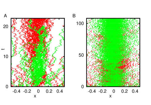
Figure 1: Examples of the dynamics of the individual-based model. In both panels, $\mu(x)$ is a Gaussian distribution with average zero and variance $\sigma=0.1$. The red species is the fastest: in both panels, $\delta D/D=0.2$ and $D=10^{-3}$. The two species are reproductively neutral, $s=0$ and are initially present at the same density. The total number density is A $N=50$ and B $N=300$. By performing several realizations of the two simulations, we find that the fixation probability of the fastest species in A is $P_{fix}\approx 0.62$ and in B is $P_{fix}\approx 0.57$.

$$\partial_{t}c_{A} = \overbrace{-\nabla[v(x)c_{A}]}^{\mathrm{Advection}}+\overbrace{(1+s)\mu(x)c_{A}}^{\mathrm{Growth}}-\overbrace{c_{A}(c_{A}+c_{B})}^{\mathrm{Competition}}+\overbrace{(D+\delta D)\nabla^{2}c_{A}}^{\mathrm{Diffusion}}+\overbrace{\sigma_{A}\xi_{B}(x,t)}^{\mathrm{Fluctuations}}$$

$$\partial_{t}c_{B} = -\nabla[v(x)c_{B}]+\qquad\mu(x)\ \ c_{B}-c_{B}(c_{A}+c_{B})+\quad\ D\nabla^{2}c_{B}\quad\ +\ \sigma_{B}\xi_{B}(x,t)$$ (1)

where $\xi_{A}(x,t)$, $\xi_{B}(x,t)$ are Gaussian, independent, delta-correlated noise sources representing demographic stochasticity. The noise amplitudes are $\sigma_{A}^{2}=c_{A}[\mu(x)+c_{A}+c_{B}]/N$ and similarly for $c_{B}$. The intraspecific and interspecific competition coefficient in Eqs. (2.1) are set to one by an appropriate choice of the density-dependent death rates and the interaction length in the individual-based model, see Pigolotti et al. (2012, 2013) and A for details.

The dynamics embodied in Eqs. (2.1) is characterized by a very rich phenomenology (Pigolotti et al., 2013). In this broad framework, we focus on the specific problem of understanding when having a larger diffusivity $\delta D>0$ confers a selective advantage or disadvantage to species $A$. We shall study this problem in different settings, where different terms in Eqs. (2.1) dominate. A possible way to analytically study the problem is the following. Consider Eqs. (2.1) and change variables to the total concentration $c_{T}(x,t)=c_{A}+c_{B}$ and the relative fraction of species $A$, $f(x,t)=c_{A}/c_{T}$. We begin by writing the equation for $c_{T}$. We always consider cases in which the difference in growth rate and diffusivities are both small, $s\ll 1$ and $\delta D/D\ll 1$. Under these approximations, $c_{T}$ evolves according to a closed equation

$$\partial_{t}c_{T}=-\nabla[v(x)c_{T}]+\mu(x)c_{T}-c_{T}^{2}+D\nabla^{2}c_{T}+\delta D\nabla^{2}c_{A}+\sqrt{\sigma^{2}_{A}+\sigma^{2}_{B}}\xi.$$ (2)

When the diffusion length scale is much smaller than the typical length scale of the gradient of $\mu(x)$ (in other words, $D\ll 1$) and the velocity field vanishes, $v(x)=0$, the stationary solution can be approximated as $c_{T}\approx\mu(x)$, i.e. the total population is close to an ideal free distribution (IFD) (Fretwell and Lucas, 1969). In the last part of the Results section, we also consider an example in which $v(x)\neq 0$ and the distribution of the total population is not necessarily close to an IFD.

Once the equilibrium value of $c_{T}$ is known, it can be substituted in the equation for the fraction $f$, which is the relevant quantity to determine which of the two species fixates. By analyzing this equation, we shall see that one can identify the effects leading to selective advantages to the fastest or the slower species.

2.2 Fixation probabilities

By repeated simulations of the individual-based model, we can estimate the fixation probability $P_{fix}$ of the fastest species for a given setting. In simple evolutionary models such as Wright-Fisher dynamics, a selective advantage biases the fixation probability according to Kimura’s formula (Kimura, 1962)

$$P_{fix}=\frac{1-e^{-Nf_{0}s}}{1-e^{-Ns}}$$ (3)

where $f_{0}$ is the initial fraction of mutants. In simple cases, the same formula holds when considering a spatially extended population (Maruyama, 1970; Whitlock, 2003; Doering et al., 2003). Examples are the stepping-stone model (Kimura and Weiss, 1964) and similar spatial models that can be described in the continuum limit by the stochastic Fisher equation

$$\partial_{t}f(x,t)=sf(1-f)+D\nabla^{2}f+\sqrt{\frac{2f(1-f)}{N}}\xi(x,t).$$ (4)

Eqs. 2.1 are more complex than (4) and it is not obvious that, in general, Eq. 3 for the fixation probability should hold. Nevertheless, we shall see that, in some cases, the equation for relative fraction of the fastest species $f$ can be cast in a form similar to Eq. (4). This allows to define an “effective” selective advantage $s_{eff}$ as the coefficient of the term proportional to $f(1-f)$ in the resulting equation.

Numerically, the effective selective advantage can be inferred from the fixation probability estimated by simulating several realizations of the individual-based model. In the simple case of an equal initial fraction of individuals of the two species, $f_{0}=1/2$, Eq. (3) can be analytically inverted, yielding

$$s_{eff}=\left\{\begin{array}[]{c}-\frac{2}{N}\log\left(\frac{1-\sqrt{1-4P_{fix}(1-P_{fix})}}{2P_{fix}}\right)\quad P_{fix}\leq\frac{1}{2}\\ -\frac{2}{N}\log\left(\frac{1+\sqrt{1-4P_{fix}(1-P_{fix})}}{2P_{fix}}\right)\quad P_{fix}>\frac{1}{2}\end{array}\right..$$ (5)

This expression allows for a direct comparison between simulations of the individual-based models and predictions of our theory. In the second part of the Results section, we will consider one case in which the nutrients are not homogeneously distributed in space. In this case, we are unaware of mathematical results ensuring that Eq. (3) and consequently Eq. (5) hold. We will check numerically that this is the case and, in particular, that no density-dependent effects appear as the initial fraction of mutants $f_{0}$ is varied.

3 Results

The effect of different diffusivities in the homogeneous case

We begin with the simple case in which the nutrient is spatially homogeneous, $\mu(x)=1$ and advecting flows are absent, $v=0$. In this case, the fastest species can take advantage of number fluctuations, as demonstrated in (Pigolotti and Benzi, 2014) and Appendix A. This subtle effect is purely due to stochasticity and is absent in the deterministic limit of $N\rightarrow\infty$.

It is interesting to analyze a case in which enhanced motility comes at the expense of a reduced reproduction rate. This setting represents a common evolutionary dilemma, where at fixed metabolic budget species have to decide how much energy to invest into movement respect to reproduction. In the general system of equations (2.1), this correspond to the choice $\delta D>0$ and $s<0$.

We proceed as described in Section 2.1. The equation for $f=c_{A}/c_{T}$ reads

$$\partial_{t}f=D\nabla^{2}f+\delta D(1-f)\nabla^{2}f+sf(1-f)+\sqrt{\frac{2f(1-f)}{N}}\xi,$$ (6)

where we already substituted the stationary value of the total concentration, $c_{T}=1$. For $|s|\ll 1$ and $\delta D/D\ll 1$, it can be shown that, on average, the term $\delta D(1-f)\nabla^{2}f$ is proportional to $\delta Df(1-f)/(ND^{3/2})$, see B and (Pigolotti and Benzi, 2014). This means that, effectively, the advantage to the fastest species due to number fluctuations is proportional to the combination of parameters $\delta D/(ND^{3/2})$. Substituting this result into (6), one obtains an equation having the same form as Eq. (4), with an effective selective advantage equal to

$$s_{eff}=s+\alpha\ \delta D/(ND^{3/2})$$ (7)

where $\alpha$ is a positive constant. The value of $\alpha$ can be mathematically estimated using different strategies. In B we summarize the calculation by Pigolotti and Benzi (2014), which is based on the continuos equation with the genetic drift. Alternatively, one can start from a discrete formulation of the same problem as done by Novak (2014). In the following, we will check the prediction of Eq. (7) and simply estimate the value of $\alpha$ numerically. Eq. (7) predicts that the effective selective advantage to the fastest species, derived the from fixation probability via Eqs. 5, must increase linearly on the combination of parameter $1/(ND^{1/2})$. We performed numerical simulations of the individual-based model at fixed value of $\delta D/D$ and $s$ and for different values of $D$ and $N$. We measured $P_{fix}$, as shown in Figure (2A), and inferred the effective selective advantage via Eqs. 5. As predicted by Eq. (7), one finds that the effective selective advantage depends linearly on the combination of parameter $1/(ND^{1/2})$, see Figure (2B). A linear fit using Eq. (7) permits to estimate the value of $\alpha\approx 0.235$.

Notice that, at increasing $N$ (or $D$), one finds a transition between a regime in which it is advantageous to diffuse faster, because of the larger demographic fluctuations, to one in which it is not convenient to pay the price of a smaller reproduction rate. Such transition is marked with a dashed line in both panels of Figure (2). We conclude this section by remarking that, in practical cases, $s$ and $\delta D$ are not independent variables. In particular, because of energy constraint, the mutants with a higher mobility $\delta D$ pay a more severe cost in terms of the difference in reproduction rate $s$. Assuming a specific functional relation between $s$ and $\delta D$, one can to obtain from Eq. (7) the optimal value of $\delta D$ by simply maximizing $s_{eff}$ under the chosen constraint.

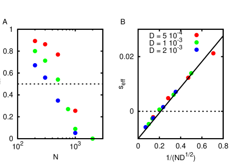
Figure 2: A Fixation probabilities at varying $N$ and $D$. In this and the following figures, error bars are either explicitly shown or smaller than the size of the symbols. B corresponding rescaling according to Eq. 7. The system is spatially homogeneous. Parameters are: $\delta D/D=0.2$. The slowest species reproduces at a slower rate, $s=-0.01$. In both panels, the dashed lines mark the transition between the regions in which diffusing faster is advantageous or disadvantageous. The continuous black line represents a linear fit of the data (see Eq. 7) with $\alpha$ as a free parameter, from which we obtain $\alpha\approx 0.235$.

Spatially inhomogeneous case

We now consider a case in which the growth rates of the two species are identical, $s=0$, but the nutrients $\mu(x)$ are not uniformly distributed in space. Also in this case, we start by deriving the dynamics for the fraction of the fast species $f$

$$\partial_{t}f=[D+(1-f)\delta D]\left[\nabla^{2}f+\frac{2(\nabla f)(\nabla c_{T})}{c_{T}}\right]+\delta Df(1-f)\frac{\nabla^{2}c_{T}}{c_{T}}+\mathrm{noise}$$ (8)

where, for small $D$, $c_{T}$ can be replaced by its stationary value $\mu(x)$ as previously discussed. The noise amplitude is $\sigma^{2}_{f}=f(1-f)[\mu(x)+c_{T}]/(Nc_{T})\approx 2f(1-f)/N$. Substituting, we obtain

$$\partial_{t}f=D\left[\nabla^{2}f+\frac{2(\nabla f)(\nabla\mu(x))}{\mu(x)}\right]+\delta D\left[(1-f)\nabla^{2}f+f(1-f)\frac{\nabla^{2}\mu(x)}{\mu(x)}\right]+\sqrt{\frac{2f(1-f)}{N}}\xi.$$ (9)

Eq. (9) is too complex to allow any analytic study. However, it is possible to understand the basic feature of the system dynamics by a reasonable interpretation of different terms in Eq. (9). The two terms in the first square brackets represent diffusion plus an effective advection term. The latter can be understood thinking that the relative concentration $f$ tends to be transported from regions of higher total density to regions of lower one. Importantly, both terms are symmetric in $f\leftrightarrow(1-f)$ and are not function of the diffusivity difference $\delta D$. Thus, they can not be directly responsible for biasing fixation probabilities towards one of the two species.

Conversely, terms in the second square brackets are proportional to the diffusivity difference $\delta D$ and thus break the symmetry between the two species. The first term is identical to that discussed in the previous section, providing a stochastic advantage to the fastest species. We assume that, also in this non-homogenous setting, its average is proportional to $\langle(1-f)\nabla^{2}f\rangle\propto f(1-f)/(ND^{3/2})$ as in the homogeneous case, where $\langle\dots\rangle$ denotes a spatial average. The second term does not depend neither on the diffusion nor on $N$. In a non-homogenous situation, the total population tends to concentrate around maxima of $\mu(x)$, where $\nabla^{2}\mu(x)<0$. This argument suggests that the average of this term over the distribution of the total population must be negative. This can be interpreted as the advantage due to the spatial inhomogeneity for the less agile species.

If the above assumptions hold, the effective selective advantage in this case is equal to

$$s_{eff}=\delta D\left[\frac{\alpha}{ND^{3/2}}+K\right].$$ (10)

where the first term in the square brackets is the noise-induced advantage discussed in the previous section, and $K<0$ is a constant related to the average value of $\nabla^{2}\mu(x)/\mu(x)$, as later discussed. As before, the balance between these two effects determines whether the fastest or the slowest species fixates with higher probability. Fixation probabilities for this model at varying $N$ and $D$ are shown in Fig. (3A). Also in this case, a one can observe a transition between regimes in which diffusing faster is advantageous or not. Equation 10 predicts that, performing simulations at fixed relative diffusivity difference, i.e. $\delta D/D=\mathrm{const}$, the quantity $s_{eff}/D$ should be a function of the combination of parameters $1/(ND^{3/2})$ only. This prediction is very well verified in the simulations, as shown in Fig. (3B).

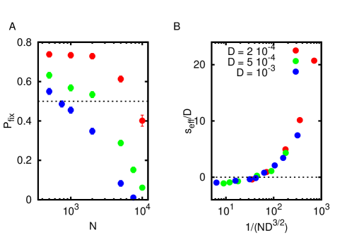
Figure 3: A Fixation probabilities in a spatially nonhomogenous system at varying $N$ and $D$ and B corresponding rescaling according to Eq. 10. The growth rate depends on space as $\mu(x)=e^{-x^{2}/(2\sigma^{2})/}\sqrt{2\pi\sigma^{2}}$. Other parameters are: $\delta D/D=0.2$, $\sigma=0.2$ and $s=0$. The dashed line in panel A marks the transition between the regions in which diffusing faster is advantageous or not.

Let us study in more details the dependence of the constant $K$ on the characteristic size of the resource patch $\sigma$ for the case in which $\mu(x)$ is Gaussian, $\mu(x)=(2\pi\sigma^{2})^{-1/2}\exp(-x^{2}/2\sigma^{2})$ . Fig. 4A shows that, indeed, the fixation probability of the fastest species increases as $\sigma$ is increased, implying that $K$ must increase (i.e. decrease in absolute value) with $\sigma$. To be more quantitative, let us focus on the term proportional to $\nabla^{2}\mu(x)/\mu(x)$ in Eq. 9

$$\delta D\left\langle f(1-f)\frac{\nabla^{2}\mu(x)}{\mu(x)}\right\rangle=\delta D\int\ dx\ f(1-f)\ \frac{x^{2}-\sigma^{2}}{\sigma^{4}}=\frac{\delta D}{\sigma}\int\ dy\ f(1-f)(y^{2}-1)$$ (11)

where $y=x/\sigma$. This calculation suggest that, at the leading order, $K$ can be estimated as $K=-\beta\ \sigma^{-1}$, where $\beta$ is a constant order $1$. This prediction is verified in Fig. 4B.

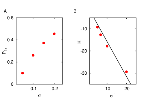
Figure 4: A Fixation probabilities in a spatially nonhomogenous system at varying the characteristic size of the resource patch $\sigma$ and corresponding effective selective advantage. Parameters are: $D=10^{-3}$, $N=10^{3}$ and $\delta D/D=0.2$. B Plot of $K=(s_{eff}/\delta D)-\alpha/(ND^{3/2})$ versus $\sigma^{-1}$ from the same data. The black line is a linear fit according to the estimate $K=-\beta\ \sigma^{-1}$, from which we obtain $\beta\approx 1.6$.

We remark that, in a spatially inhomogeneous system, the fixation formula of Eq. 3 is not guaranteed to be valid as non-homogeneities could potentially lead to a density-dependent selective advantage. To check this possibility, we studied the dependence of the fixation probability as a function of the initial fraction of mutants. The results in Fig. 5 shows that, choosing spatially homogeneous initial conditions but at different initial fraction $f_{0}$, fixation probabilities are very well described by Kimura’s formula also in this scenario. This confirms that density-dependent effects are absent or unimportant.

Figure 5: Fixation probabilities in a spatially nonhomogenous system as a function of the initial fraction of mutants $f_{0}$. For all values of $f_{0}$, individuals of $A$ and $B$ are uniformly distributed in space at $t=0$. The continuous line is the prediction of Kimura’s formula, Eq. 3. The effective selective advantage $s_{eff}\approx 0.0043$ has been obtained via a fitting procedure. Parameters are: $D=2\ 10^{-4}$, $N=500$, $\sigma=0.2$ and $\delta D/D=0.2$.

Advection

In this section, we study the combined effect of a non-uniform growth rate $\mu(x)=\exp[-x^{2}/(2\sigma^{2})]$ and a velocity field $v(x)=-\gamma x$ attracting individuals toward the point $x=0$.

This velocity field can be thought of as a simple example of the behavior close to sinks of a turbulent velocity field (Pigolotti et al., 2012). Indeed, although three-dimensional velocity fields in the ocean are obviously incompressible, additional forces such as gyrotaxis on small scales Durham et al. (2013) or upwelling/downwelling on larger scales Benzi et al. (2012) can be taken into account by considering in an “effective” compressible velocity field experienced by microorganisms.

For simplicity, we start by analyzing the problem in the absence of demographic fluctuations, $N\rightarrow\infty$. Proceeding as before, we obtain an equation for $f$:

$$\partial_{t}+v(x)\nabla f=(D+\delta D)\Delta f+2(D+\delta D)[\nabla\log(c_{T})]\nabla f+\delta D\Delta f(1-f)+\frac{\Delta c_{T}}{c_{T}}f(1-f).$$ (12)

It is useful to notice that both $\mu(x)$ and $v(x)$ effectively concentrate the total population $c_{T}$ in a limited region of space. In particular, for small values of $D$ and in the absence of the velocity field, we argued that the non-homogeneous nutrient distribution would lead to a total population density $c_{T}\approx\mu(x)$. The velocity field alone would concentrate $c_{T}$ in a similar way, leading to $c_{T}\propto\exp[-\gamma x^{2}/(2D)]$.

However, the characteristic spatial scale at which the population is concentrated by the two effects is different: $\sigma$ for non-homogenous $\mu(x)$ and $l\equiv\sqrt{D/\gamma}$ for the velocity field. It can be expected that the effect of $\delta D$ would depend on the adimensional ratio $r\equiv l/\sigma$ of these two different scales, controlling which of these two effects dominates. For $r\ll 1$, the velocity field controls the width of the total population. In this case, the species diffusing faster has a selective advantage, as it can invade more easily upstream regions and therefore invade the system (Pigolotti et al., 2012). For $r\gg 1$, the dominant effect is given by the non-homogeneous nutrient distribution. In this case, the faster species has a selective disadvantage, for the argument presented in previous section. An analytical argument obtained by expanding the function $f$ around the point $x=0$ support the fact that the transition should occur exactly at $r=1$, see Appendix B.

Figure 6: Dynamics in the presence of an advective linear field. Parameters are $D=10^{-3}$, $\delta D/D=0.2$, $\sigma=0.1$. The ratio of length scales $r$ is varied by tuning $\gamma$.The dashed line marks the transition between a selective advantage and a disadvantage to the fastest species.

The transition between these two regimes can be observed in the numerical simulations of figure (6). For large population size (red dots), one observe a behavior very close to the theoretical prediction, although the transition seems to occur at a value of $r$ slightly smaller than one. For smaller population size (blue dots) the transition is more smoothed, as noise plays a more important role in this case. Notice also that, for large $r$, the fixation probability of the fast species is significantly larger than zero. This is due to the previously discussed stochastic advantage for the fast species which also acts in this case.

Following Novak (2014), the transition at $r=1$ can also be interpreted by considering which of the two populations is closer to an IFD. In our notation, a population characterized by a diffusivity $D$ is at an IFD under the condition of balanced dispersal (Doncaster et al., 1997; Cantrell et al., 2010; Novak, 2014)

$$D\nabla^{2}\mu(x)+\nabla[v(x)\mu(x)]=0.$$ (13)

which is satisfied only when $\gamma=1/\sigma^{2}$ and $r=1$. For $r<1$, the population with higher value of $D$ is closer to an IFD and therefore has a selective advantage. Conversely, for $r>1$ an increase of diffusivity leads to a larger deviation from an IFD, therefore to a decrease in the fixation probability.

4 Discussion

In this paper, we studied competition between two populations having different diffusivities. We have shown how the ecological forces acting on the populations, including non-homogeneities in the resource distributions and transport by fluid flows, determine the best competitor in a non-trivial way. All these ingredients can be systematically analyzed by means of macroscopic stochastic equations describing the evolution of the two populations in space and time. This approach allows for explicitly estimate the effective selective advantage, or disadvantage, granted by diffusing faster in a given ecological settings.

The three examples discussed in this paper present different tradeoffs between two ecological forces, one promoting diffusion and one contrasting it. Our first example was contrasting demographic stochasticity, giving an advantage to the fastest species, with a slower reproduction rate. In the second case, we contrasted demographic stochasticity with a non-homogenous nutrient distribution, where the latter confers an advantage to the slowest species. We concluded with a case in which non-homogeneity in the nutrients is contrasted with a fluid flow concentrating individuals around a velocity sink. In this latter case, diffusing faster constitutes an advantage as faster individuals can colonize more easily upstream regions, from which they can invade.

These three examples fit into a more general theoretical scheme. In the absence of demographic stochasticity, or other temporal fluctuations, evolution tends to advantage the level of dispersal that brings the population close to an IFD Novak (2014). In the absence of fluid transport, this implies that the species diffusing less is always more fit (Hastings, 1983; Dockery et al., 1998). However, this is not necessarily the case in the presence of intense fluid flows, where the fastest species is closer to an IFD. Further, taking into account demographic stochasticity does not only make the outcome of competition more uncertain, as in classic examples of competing species having different reproduction rates (Kimura, 1962); it also confers an additional advantage to the species diffusing faster. This observation is consistent with previous studies (Kessler and Sander, 2009; Waddell et al., 2010; Lin et al., 2014; Pigolotti and Benzi, 2014; Lin et al., 2015). This effect is already appreciable for differences in diffusivities of a few percent. While we focused for simplicity on one spatial dimension, analytical and numerical studies show that the effect becomes even stronger as spatial dimension is increased (Pigolotti and Benzi, 2014). Overall, these results challenge the view that in time-independent environments it is always convenient to diffuse less (Hastings, 1983; Dockery et al., 1998) and suggest that deterministic models can miss a crucial ingredient to determine the best dispersal strategy.

It is tempting to interpret the stochastic advantage to fast species discussed here to the classic argument by Hamilton and May (1977), according to which the advantage of diffusing faster is related to avoidance of competition with conspecific. Indeed, demographic stochasticity is one of the main ingredients of Hamilton and May’s seed dispersal model. It should however be noted that, in the context of the model presented in this paper, the intensity of intraspecific competition is the same for both species because of symmetry. After neglecting fluctuations of the total density, interspecific competition depends only on the relative fraction of the two species and not on their diffusivity. It is therefore not obvious whether one can interpret the stochastic advantage of diffusing faster in our model in terms of a reduced interspecific competition.

Other effects not discussed in this paper can be understood by means of similar arguments. For example, in population models where a pattern-forming transition organizes species in spatial clusters, there is a tendency of slower species to be the best competitors (Hernández-García and López, 2004; Heinsalu et al., 2013; Hernández-García et al., 2014). This phenomenon is resemblant to the case of non-homogeneous nutrients. In both cases, a non-homogeneous carrying capacity confers an advantage to less motile species, although in this case the non-homonogeneity is not explicit but rather due to an instability of the homogeneous state.

We thank C. Doering and E. Hernandez-Garcia for useful discussions. SP acknowledges partial support from Spanish Ministry of Economy and Competitiveness and FEDER (project FIS2012-37655-C02-01).

Appendix A Individual-based model

In this Appendix, we discuss details of the implementation of the individual-based model. Individual belonging to the two species are treated as point-like particles in a one-dimensional space. The coordinate $x$ of of any given particle evolves according to the Langevin dynamics

$$\dot{x}=v(x)+\sqrt{2D_{A,B}}\ \xi(t)$$ (14)

where $v(x)$ is a velocity field, different from zero only in the case of Section (3). $D_{A,B}$ is the diffusivity which depends on the species ($A$ or $B$) and $\xi(t)$ is a white noise.

In addition, particles can be created (birth event) or removed (death event) stochastically. Each individual of species $A$ reproduces at rate $\mu(x)$, while each individual of species $B$ reproduces at rate $\mu(x)(1+s)$ where $s$ is a selective advantage. Newborn individuals are placed at the same coordinate as their mother. Defining the interaction distance $\delta$ eath event occur at a rate $\tilde{n}_{A}+\tilde{n}_{B}$, where $\tilde{n}_{A,B}$ are the number of individuals found at a distance less than $\delta$ from each individual. Dead individuals are simply removed from the system. See (Perlekar et al., 2011) for further details on the numerical implementation.

It can be shown that the parameter $\delta$ can be used to tune the average number of individuals. In particular, defining $\delta=1/N$ and $c_{A,B}(x)=n_{A,B}(x)/N$ where $=n_{A,B}(x)$ is the number density of individuals, one can derive from the individual-based model the macroscopic Eqs. (2.1), see Pigolotti et al. (2012, 2013).

Appendix B Stochastic advantage of diffusing faster in homogeneous environments

In this Appendix, we briefly recall the main result of Pigolotti and Benzi (2014). Our starting point is the one-dimensional stochastic differential equation

$$\partial_{t}f=D\nabla^{2}f+\delta D(1-f)\nabla^{2}f+\sigma\xi$$ (15)

with $\sigma=\sqrt{2\mu f(1-f)/N}$. Calling $\langle\dots\rangle$ the average over space and noise and averaging Eq. (15) leads to

$$\frac{d\ \langle f\rangle}{dt}=\langle(\nabla f)^{2}\rangle.$$ (16)

Since the right hand side of Eq. (16) is always non-negative, one can already conclude that the average effect of having a larger diffusivity is advantageous. We can rewrite Eq. (16) in terms of the heterozygosity function, $H(d,t)=\langle f(x)[1-f(x+d)]+f(x+d)[1-f(x)]\rangle$. After some simple algebra we get

$$\frac{d\ \langle f\rangle}{dt}=\frac{\delta D}{2}\frac{\partial^{2}}{\partial d^{2}}H(d,t)|_{d=0}.$$ (17)

Eq. (17) is an exact relation between the average growth of the density of the fastest species and the heterozygosity. To make progress, we assume $\delta D/D\ll 1$. In this limit, we can estimate the right hand side of Eq. (17) at first order in perturbation theory, i.e. by approximating the heterozygosity with that calculated in the purely neutral case of $\delta D=0$, which is explicitly known, see e.g. Korolev et al. (2010). Under this approximation, we finally obtain

$$\frac{dF(t)}{dt}=\frac{\delta D}{4D\sqrt{\pi\epsilon t_{f}}}H(0,0){G(t/t_{f})}$$ (18)

where $G(x)=\exp(x)\mathrm{erfc}(\sqrt{x})$ and $t_{f}=2DN^{2}$. The parameter $\epsilon$ is a constant with the dimension of a time and on the order of the smallest time-scale of the system, i.e. the generation time $\epsilon\approx\mu^{-1}$. Proceeding in the same way for the stochastic Fisher equation, one would obtain $dF/dt=sH(0,0)G(t/t_{f})/2$. By comparing this expression and Eq. 18, we can finally define an effective selective advantage

$$s_{eff}=\frac{\alpha\delta D}{ND^{3/2}}$$ (19)

where we defined the constant $\alpha=(2\sqrt{2\pi\epsilon})^{-1}$.

Appendix C Transition in a velocity sink

In this section, we present an approximate theory for the results of Fig. (6). We assume that the important region to study is near $x=0$, where the relative density of the fast species can be approximated as $f(x)\approx f_{0}+f_{1}x^{2}$. We substitute this assumption in (12) and disregard all terms $o(x^{4})$. We also assume $c_{T}=\mu(x)$, which is a good approximation near the point $r=1$. Equating terms of the same order in $x$ leads to the system of differential equations

$${\dot{f}_{0}} = 2Df_{1}+2\delta Df_{1}(1-f_{0})-\delta Df_{0}(1-f_{0})$$ (20)

$${\dot{f}_{1}} = 2\Gamma f_{1}-(4D+5\delta D)\frac{f_{1}}{\sigma^{2}}-2\delta Df_{1}^{2}+\frac{\delta D}{\sigma^{2}}f_{1}f_{0}+\frac{\delta D}{\sigma^{4}}f_{0}(1-f_{0})$$ (21)

This system admits two fixed points, $(f_{0},f_{1})$, equal to $(0,0)$ and $(1,0)$, corresponding to fixation of one of the two species respectively. Let us study the stability of the point $0,0$. The eigenvalues $\lambda_{i}$ of the linear stability analysis are

$$\lambda_{1} = \frac{1}{\sigma^{2}}\left[2D(\xi-2)+6\delta D+\delta D\frac{1-\xi}{2-\xi}\right]$$ (22)

$$\lambda_{2} = -\frac{\delta D}{\sigma^{2}}\frac{1-\xi}{2-\xi}$$ (23)

where $\xi=\gamma\sigma^{2}/D=r^{-2}$. While $\lambda_{1}<0$ for small $\delta D/D$ and $\xi\approx 1$, $\lambda_{2}$ becomes positive at $\xi>1$, where the stable fixed point becomes $1,0$. This analysis explains the transition observed close to $r=1$ in figure (6).

References

- Benzi et al. (2012) Benzi, R., Jensen, M. H., Nelson, D. R., Perlekar, P., Pigolotti, S., Toschi, F., 2012. Population dynamics in compressible flows. The European Physical Journal Special Topics 204 (1), 57–73.
- Bianco et al. (2014) Bianco, G., Mariani, P., Visser, A. W., Mazzocchi, M. G., Pigolotti, S., 2014. Analysis of self-overlap reveals trade-offs in plankton swimming trajectories. Journal of The Royal Society Interface 11 (96), 20140164.
- Cantrell et al. (2010) Cantrell, R. S., Cosner, C., Lou, Y., 2010. Evolution of dispersal and the ideal free distribution. Mathematical biosciences and engineering: MBE 7 (1), 17–36.
- Comins et al. (1980) Comins, H. N., Hamilton, W. D., May, R. M., 1980. Evolutionarily stable dispersal strategies. Journal of theoretical Biology 82 (2), 205–230.
- Dieckmann et al. (1999) Dieckmann, U., O’Hara, B., Weisser, W., 1999. The evolutionary ecology of dispersal. Trends in Ecology & Evolution 14 (3), 88–90.
- Dockery et al. (1998) Dockery, J., Hutson, V., Mischaikow, K., Pernarowski, M., 1998. The evolution of slow dispersal rates: a reaction diffusion model. Journal of Mathematical Biology 37 (1), 61–83.
- Doering et al. (2003) Doering, C. R., Mueller, C., Smereka, P., 2003. Interacting particles, the stochastic fisher–kolmogorov–petrovsky–piscounov equation, and duality. Physica A: Statistical Mechanics and its Applications 325 (1), 243–259.
- Doncaster et al. (1997) Doncaster, C. P., Clobert, J., Doligez, B., Danchin, E., Gustafsson, L., 1997. Balanced dispersal between spatially varying local populations: an alternative to the source-sink model. The American Naturalist 150 (4), 425–445.
- Durham et al. (2013) Durham, W. M., Climent, E., Barry, M., De Lillo, F., Boffetta, G., Cencini, M., Stocker, R., 2013. Turbulence drives microscale patches of motile phytoplankton. Nature communications 4.
- Fretwell and Lucas (1969) Fretwell, S. D., Lucas, H. R., 1969. On territorial behavior and other factors influencing habitat distribution of birds. Acta Biotheoretica 19, 16–36.
- Hamilton and May (1977) Hamilton, W. D., May, R. M., 1977. Dispersal in stable habitats. Nature 269 (5629), 578–581.
- Hastings (1983) Hastings, A., 1983. Can spatial variation alone lead to selection for dispersal? Theoretical Population Biology 24 (3), 244–251.
- Heinsalu et al. (2013) Heinsalu, E., Hernández-Garcia, E., López, C., 2013. Clustering determines who survives for competing brownian and lévy walkers. Physical review letters 110 (25), 258101.
- Hernández-García et al. (2014) Hernández-García, E., Heinsalu, E., Lopez, C., 2014. Spatial patterns of competing random walkers. Ecological Complexity.
- Hernández-García and López (2004) Hernández-García, E., López, C., 2004. Clustering, advection, and patterns in a model of population dynamics with neighborhood-dependent rates. Physical Review E 70 (1), 016216.
- Kessler and Sander (2009) Kessler, D. A., Sander, L. M., 2009. Fluctuations and dispersal rates in population dynamics. Physical Review E 80 (4), 041907.
- Kimura (1962) Kimura, M., 1962. On the probability of fixation of mutant genes in a population. Genetics 47 (6), 713.
- Kimura and Weiss (1964) Kimura, M., Weiss, G. H., 1964. The stepping stone model of population structure and the decrease of genetic correlation with distance. Genetics 49 (4), 561.
- Korolev et al. (2010) Korolev, K., Avlund, M., Hallatschek, O., Nelson, D. R., 2010. Genetic demixing and evolution in linear stepping stone models. Reviews of modern physics 82 (2), 1691.
- Lin et al. (2014) Lin, Y. T., Kim, H., Doering, C. R., 2014. Demographic stochasticity and evolution of dispersion i. spatially homogeneous environments. Journal of mathematical biology, 1–32.
- Lin et al. (2015) Lin, Y. T., Kim, H., Doering, C. R., 2015. Demographic stochasticity and evolution of dispersion ii: Spatially inhomogeneous environments. Journal of mathematical biology 70 (3), 679–707.
- Maruyama (1970) Maruyama, T., 1970. Effective number of alleles in a subdivided population. Theoretical population biology 1 (3), 273–306.
- Novak (2014) Novak, S., 2014. Habitat heterogeneities versus spatial type frequency variances as driving forces of dispersal evolution. Ecology and evolution 4 (24), 4589–4597.
- Perlekar et al. (2011) Perlekar, P., Benzi, R., Pigolotti, S., Toschi, F., 2011. Particle algorithms for population dynamics in flows. In: Journal of Physics: Conference Series. Vol. 333. IOP Publishing, p. 012013.
- Pigolotti and Benzi (2014) Pigolotti, S., Benzi, R., 2014. Selective advantage of diffusing faster. Physical review letters 112 (18), 188102.
- Pigolotti et al. (2012) Pigolotti, S., Benzi, R., Jensen, M. H., Nelson, D. R., 2012. Population genetics in compressible flows. Physical review letters 108 (12), 128102.
- Pigolotti et al. (2013) Pigolotti, S., Benzi, R., Perlekar, P., Jensen, M. H., Toschi, F., Nelson, D., 2013. Growth, competition and cooperation in spatial population genetics. Theoretical population biology 84, 72–86.
- Purcell (1977) Purcell, E. M., 1977. Life at low reynolds number. Am. J. Phys 45 (1), 3–11.
- Visser et al. (2009) Visser, A. W., Mariani, P., Pigolotti, S., 2009. Swimming in turbulence: zooplankton fitness in terms of foraging efficiency and predation risk. Journal of Plankton Research 31 (2), 121–133.
- Waddell et al. (2010) Waddell, J. N., Sander, L. M., Doering, C. R., 2010. Demographic stochasticity versus spatial variation in the competition between fast and slow dispersers. Theoretical population biology 77 (4), 279–286.
- Whitlock (2003) Whitlock, M. C., 2003. Fixation probability and time in subdivided populations. Genetics 164 (2), 767–779.