Simple and Efficient Fully-Functional Succinct Trees

Abstract

The fully-functional succinct tree representation of Navarro and Sadakane (ACM Transactions on Algorithms, 2014) supports a large number of operations in constant time using $2n+o(n)$ bits. However, the full idea is hard to implement. Only a simplified version with $\mathcal{O}\!\left(\lg n\right)$ operation time has been implemented and shown to be practical and competitive. We describe a new variant of the original idea that is much simpler to implement and has worst-case time $\mathcal{O}\!\left(\lg\lg n\right)$ for the operations. An implementation based on this version is experimentally shown to be superior to existing implementations.

1 Introduction

Combinatorial arguments show that it is possible to represent any ordinal tree of $n$ nodes using less than $2n$ bits of space: the number of such trees is the $(n-1)$th Catalan number, $\frac{1}{n}{2n-2\choose n-1}$, and its logarithm (in base 2 and written $\lg$ across this paper) is $2n-\Theta(\lg n)$. A simple way to encode any ordinal tree in $2n$ bits is the so-called balanced parentheses (BP) representation: traverse the tree in depth-first order, writing an opening parenthesis upon reaching a node, and a closing one upon definitely leaving it. Much more challenging is, however, to efficiently navigate the tree using that representation.

The interest in navigating a $2n$-bit representation of a tree, compared to using a classical $\mathcal{O}\!\left(n\right)$-pointers representation, is that those succinct data structures allow fitting much larger datasets in the faster and smaller levels of the memory hierarchy, thereby improving the overall system performance. Note that compression is not sufficient; it must be possible to operate the data in its compressed form. The succinct representation of ordinal trees is one of the most clear success stories in this field. Table 1 lists the operations that can be supported in constant time within $2n+o(n)$ bits of space. These form a rich set that suffices for most applications.

Table 1: Operations on ordinal trees, where $i$ and $j$ are node identifiers.

operation	description
$\mathit{root}$	the tree root
$\mathit{preorder}(i)$ / $\mathit{postorder}(i)$	preorder/postorder rank of node $i$
$\mathit{preorderselect}(k)$ / $\mathit{postorderselect}(k)$	the node with preorder/postorder $k$
$\mathit{isleaf}(i)$	whether the node is a leaf
$\mathit{isancestor}(i,j)$	whether $i$ is an ancestor of $j$
$0pt(i)$	depth of node $i$
$\mathit{parent}(i)$	parent of node $i$
$\mathit{fchild}(i)$ / $\mathit{lchild}(i)$	first/last child of node $i$
$\mathit{nsibling}(i)$ / $\mathit{psibling}(i)$	next/previous sibling of node $i$
$\mathit{subtree}(i)$	number of nodes in the subtree of node $i$
$\mathit{levelancestor}(i,d)$	ancestor $j$ of $i$ such that $0pt(j)=0pt(i)-d$
$\mathit{levelnext}(i)$ / $\mathit{levelprev}(i)$	next/previous node of $i$ with the same depth
$\mathit{levelleftmost}(d)$ / $\mathit{levelrightmost}(d)$	leftmost/rightmost node with depth $d$
$\mathit{lca}(i,j)$	the lowest common ancestor of two nodes $i,j$
$\mathit{deepestnode}(i)$	the (first) deepest node in the subtree of $i$
$0pt(i)$	the height of $i$ (distance to its deepest node)
$\mathit{degree}(i)$	$q=$ number of children of node $i$
$\mathit{child}(i,q)$	$q$-th child of node $i$
$\mathit{childrank}(i)$	$q=$ number of siblings to the left of node $i$
$\mathit{leafrank}(i)$	number of leaves to the left and up to node $i$
$\mathit{leafselect}(k)$	$k$th leaf of the tree
$\mathit{numleaves}(i)$	number of leaves in the subtree of node $i$
$\mathit{leftmostleaf}(i)$ / $\mathit{rightmostleaf}(i)$	leftmost/rightmost leaf of node $i$

The story starts with Jacobson [10], who proposed a simple levelwise representation called LOUDS, which reduced tree navigation to two simple primitives on bitvectors: $\mathit{rank}$ and $\mathit{select}$ (all these primitives will be defined later). However, the repertoire of tree operations was limited. Munro and Raman [15] used for the first time the BP representation, and showed how three basic primitives on the parentheses: $\mathit{open}$, $\mathit{close}$, and $\mathit{enclose}$, plus $\mathit{rank}$ and $\mathit{select}$, were sufficient to support a significantly wider set of operations. The operations were supported in constant time, however the solution was quite complex in practice. Geary et al. [8] retained constant times with a much simpler solution to $\mathit{open}$, $\mathit{close}$, and $\mathit{enclose}$, based on a two-level recursion scheme. Still, not all the operations of Table 1 were supported. Missing ones were added one by one: $\mathit{children}$ [5], $\mathit{levelancestor}$ [14], $\mathit{child}$, $\mathit{childrank}$, $0pt$, and $\mathit{lca}$ [13]. Each such addition involved extra $o(n)$-bit substructures that were also hard to implement.

An alternative to BP, called DFUDS, was introduced by Benoit et al. [4]. It also used $2n$ balanced parentheses, but they had a different interpretation. Its main merit was to support $\mathit{child}$ and related operations very easily and in constant time. It did not support, however, operations $\mathit{childrank}$, $0pt$, $\mathit{levelancestor}$, and $\mathit{lca}$, which were added later [9, 11], again each using $o(n)$ bits and requiring a complex implementation to achieve constant time.

Navarro and Sadakane [16] introduced a new representation based on BP, said to be fully-functional because it supported all of the operations in Table 1 in constant time and using a single set of structures. This was a significant simplification of previous results and enabled the development of an efficient implementation. The idea was to reduce all the tree operations to a small set of primitives over parentheses: $\mathit{fwdsearch}$, $\mathit{bwdsearch}$, $\mathit{rmq}$, and a few variations. The main structure to implement those primitives was the so-called range min-max tree (rmM-tree), which is a balanced tree of arity $\lg^{\epsilon}n$ (for a constant $0<\epsilon<1$) that supports the primitives in constant time on buckets of $\mathcal{O}\!\left(\mathop{\mathrm{polylog}}n\right)$ parentheses. To handle queries that were not solved within a bucket, other structures had to be added, and these were far less simple.

A simple $\mathcal{O}\!\left(\lg n\right)$-time implementation using a single binary range min-max tree for the whole sequence [1] was shown to be faster (or use much less space, or both) than other implementable constant-time representations [8] in several real-life trees and navigation schemes. Only the LOUDS representation was shown to be competitive, within its limited functionality. While the $\mathcal{O}\!\left(\lg n\right)$ growth was shown to be imperceptible in many real-life traversals, some stress tests pursued later [12] showed that it does show up in certain plausible situations.

No attempt was made to implement the actual constant-time proposal [16]. The reason is that, while constant-time and $o(n)$-bit space in theory, the structures used for inter-bucket queries, as well as the variant of rmM-trees that operates in constant time, involve large constants and include structures that are known to be hard to implement efficiently, such as fusion trees [7] and compressed bitvectors with optimal redundancy [18]. Any practical implementation of these ideas leads again to the $\mathcal{O}\!\left(\lg n\right)$ times already obtained with binary rmM-trees.

In this paper we introduce an alternative construction that builds on binary rmM-trees and is simple to implement. It does not reach constant times, but rather $\mathcal{O}\!\left(\lg\lg n\right)$ time, and requires $2n+\mathcal{O}\!\left(n/\lg n\right)$ bits of space. We describe a new implementation building on these ideas, and experimentally show that it outperforms a state-of-the-art implementation of the $O(\lg n)$-time solution, both in time and space, and therefore becomes the new state-of-the art implementation of fully-functional succinct trees.

2 Basic Concepts

2.1 Bits and balanced parentheses

Given a bitvector $B[1,2n]$, we define $\mathit{rank}_{t}(i)$ as the number of occurrences of the bit $t$ in $B[1,i]$. We also define $\mathit{select}_{t}(k)$ as the position in $B$ of the $k$th occurrence of the bit $t$. Both primitives can be implemented in constant time using $o(n)$ bits on top of $B$ [6]. Note that $\mathit{rank}_{1}(i)+\mathit{rank}_{0}(i)=i$ and $\mathit{rank}_{t}(\mathit{select}_{t}(k))=k$.

A sequence of $2n$ parentheses will be represented as a bitvector $B[1,2n]$ by interpreting ‘(’ as a 1 and ‘)’ as a 0. On such a sequence we define the operation $\mathit{excess}(i)$ as the number of opening minus closing parentheses in $B[1,i]$, that is, $\mathit{excess}(i)=\mathit{rank}_{1}(i)-\mathit{rank}_{0}(i)=2\mathit{rank}_{1}(i)-i$. We say that $B$ is balanced if $\mathit{excess}(i)\geq 0$ for all $i$, and $\mathit{excess}(2n)=0$. Note that $\mathit{excess}(i)=\mathit{excess}(i-1)\pm 1$.

In a balanced sequence, every opening parenthesis at $B[i]$ has a matching closing parenthesis at $B[j]$ for $j>i$, and every other parenthesis opening inside $B[i+1,j-1]$ has its matching parenthesis inside $B[i+1,j-1]$ as well. Thus the parentheses define a hierarchy. Moreover, we have $\mathit{excess}(j)=\mathit{excess}(i)-1$ and $\mathit{excess}(m)\geq\mathit{excess}(i)$ for all $i<m<j$. This motivates the definition of the following primitives on parentheses [15]:

$\mathit{close}(i)$:

the position of the closing parenthesis that matches $B[i]=1$, that is, the smallest $j>i$ such that $\mathit{excess}(j)=\mathit{excess}(i)-1$.

$\mathit{open}(i)$:

the position of the opening parenthesis that matches $B[i]=0$, that is, the largest $j<i$ such that $\mathit{excess}(j-1)=\mathit{excess}(i)$.

$\mathit{enclose}(i)$:

the opening parenthesis of the smallest matching pair that contains position $i$, that is, the largest $j<i$ such that $\mathit{excess}(j-1)=excess(i)-2$.

It turns out that a more general set of primitives is useful to implement a large number of tree operations [16], which look forward or backward for an arbitrary relative excess:

$$\mathit{fwdsearch}(i,d) \!=\! \min\{j>i,~{}\mathit{excess}(j)=excess(i)+d\},$$

$$\mathit{bwdsearch}(i,d) \!=\! \max\{j<i,~{}\mathit{excess}(j)=excess(i)+d\}.$$

In particular, we have $\mathit{close}(i)=\mathit{fwdsearch}(i,-1)$, $\mathit{open}(i)=\mathit{bwdsearch}(i,0)+1$, and $\mathit{enclose}(i)=\mathit{bwdsearch}(i,-2)+1$.

To implement other tree operations, we also need the following primitives, which refer to minimum and maximum excess in a range of $B$:

$\mathit{rmq}(i,j)$:

position of the leftmost minimum in $\mathit{excess}(i)$, $\mathit{excess}(i+1),\ldots,\mathit{excess}(j)$.

$\mathit{rMq}(i,j)$:

position of the leftmost maximum in $\mathit{excess}(i)$, $\mathit{excess}(i+1),\ldots,\mathit{excess}(j)$.

$\mathit{mincount}(i,j)$:

number of occurrences of the minimum in $\mathit{excess}(i)$, $\mathit{excess}(i+1),\ldots,\mathit{excess}(j)$.

$\mathit{minselect}(i,j,q)$:

position of the $q$th minimum in $\mathit{excess}(i)$, $\mathit{excess}(i+1),\ldots,\mathit{excess}(j)$.

2.2 BP representation of ordinal trees

As said in the Introduction, an ordinal tree of $n$ nodes is represented with $2n$ parentheses by opening a parenthesis when we arrive at a node and closing it when we leave the node. The resulting sequence is balanced, and the hierarchy it defines corresponds to subtree containment. Let us identify each node with the position of its opening parenthesis in the sequence $B$. See Figure 1.

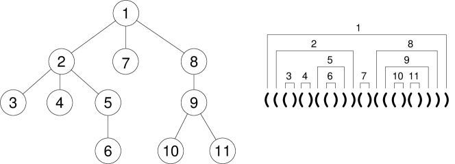
Figure 1: An ordinal tree on the left (the node identifiers are their preorder numbers) and its BP representation on the right, indicating which parentheses represent each node. For example the node with preorder 5 has identifier 7, which is its position in the sequence of parentheses.

Many tree operations are immediately translated into the primitives we have defined [15]: $\mathit{root}=1$, $0pt(i)=\mathit{excess}(i)$, $\mathit{parent}(i)=\mathit{enclose}(i)$, $\mathit{isleaf}(i)$ iff $B[i+1]=0$, $\mathit{fchild}(i)=i+1$ (if $i$ is not a leaf), $\mathit{nsibling}(i)=\mathit{close}(i)+1$ (if the result $j$ holds $B[j]=0$ then $i$ has no next sibling), $\mathit{psibling}(i)=\mathit{open}(i-1)$ (if $B[i-1]=1$ then $i$ has no previous sibling), $\mathit{lchild}(i)=\mathit{open}(\mathit{close}(i)-1)$ (if $i$ is not a leaf), $\mathit{preorder}(i)=\mathit{rank}_{1}(i)$, $\mathit{preorderselect}(k)=\mathit{select}_{1}(k)$, $\mathit{postorder}(i)=\mathit{rank}_{0}(\mathit{close}(i))$, $\mathit{postorderselect}(k)=\mathit{open}(\mathit{select}_{0}(k))$, $\mathit{isancestor}(i,j)$ iff $i\leq j<\mathit{close}(i)$, and $\mathit{subtree}(i)=(\mathit{close}(i)-i+1)/2$.

The primitives $\mathit{fwdsearch}$ and $\mathit{bwdsearch}$ yield other tree operations [16]: $\mathit{levelancestor}(i,d)=\mathit{bwdsearch}(i,-d-1)+1$, $\mathit{levelnext}(i)=\mathit{fwdsearch}(\mathit{close}(i),1)$, $\mathit{levelprev}(i)=\mathit{open}(\mathit{bwdsearch}(i,0)+1)$, $\mathit{levelleftmost}(d)=\mathit{fwdsearch}(0,d)$, and $\mathit{levelrightmost}(d)=\mathit{open}(\mathit{bwdsearch}(2n+1,d))$. The other primitives yield the remaining operations: $\mathit{degree}(i)=\mathit{mincount}(i+1,\mathit{close}(i)-1)$, $\mathit{child}(i,q)=\mathit{minselect}(i+1,\mathit{close}(i)-1,q-1)+1$ for $q>1$ (for $q=1$ it is $\mathit{fchild}(i)$), $\mathit{childrank}(i)=\mathit{mincount}(\mathit{parent}(i)+1,i)+1$ unless $B[i-1]=1$ (in which case $\mathit{childrank}(i)=1$), $\mathit{lca}(i,j)=\mathit{parent}(\mathit{rmq}(i,j)+1)$ unless $\mathit{isancestor}(i,j)$ (so $\mathit{lca}(i,j)=i$) or $\mathit{isancestor}(j,i)$ (so $\mathit{lca}(i,j)=j$), $\mathit{deepestnode}(i)=\mathit{rMq}(i,\mathit{close}(i))$, and $0pt(i)=\mathit{excess}(\mathit{deepestnode}(i))-\mathit{excess}(i)$.

Finally, the operations on leaves are solved by extending the bitvector $\mathit{rank}$ and $\mathit{select}$ primitives to count the occurrences of pairs $10$ (which represent tree leaves, ‘()’): $\mathit{rank}_{10}(i)$ is the number of occurrences of $10$ starting in $B[1,i]$ and $\mathit{select}_{10}(k)$ is the position of the $k$th occurrence of $10$ in $B$. These are easily implemented as extensions of the basic $\mathit{rank}$ and $\mathit{select}$ primitives, adding other $o(n)$ bits on top of $B$. Then $\mathit{leafrank}(i)=\mathit{rank}_{10}(i)$, $\mathit{leafselect}(k)=\mathit{select}_{10}(k)$, $\mathit{numleaves}(i)=\mathit{leafrank}(\mathit{close}(i))-\mathit{leafrank}(i-1)$, $\mathit{leftmostleaf}(i)=\mathit{leafselect}(\mathit{leafrank}(i-1)+1)$ and finally $\mathit{rightmostleaf}(i)=\mathit{leafselect}(\mathit{leafrank}(\mathit{close}(i)))$.

Therefore, all the operations of Table 1 are supported via the primitives $\mathit{fwdsearch}$, $\mathit{bwdsearch}$, $\mathit{rmq}$, $\mathit{rMq}$, $\mathit{mincount}$, and $\mathit{minselect}$. We also need $\mathit{rank}$ and $\mathit{select}$ on 0, 1, and 10.

2.3 Range min-max trees

We describe the simple version of the structure used by Navarro and Sadakane [16] to solve the primitives. We choose a block size $b$. Then, the (binary) range min-max tree, or rmM-tree, of $B[1,2n]$ is a complete binary tree where the $k$th leaf covers $B[(k-1)b+1,kb]$. Each rmM-tree node $v$ stores the following fields: $v.e$ is the total excess of the area covered by $v$, $v.m$ is the minimum excess in this area, $v.M$ is the maximum excess in the area, and $v.n$ is the number of times the minimum excess occurs in the area. Since the rmM-tree is complete, it can be stored without pointers, like a heap. See Figure 2.

Figure 2: The rmM-tree of the parentheses sequence of Figure 1. The numbers below are $\mathit{excess}(i)$.

Then, an operation like $\mathit{fwdsearch}(i,d)$ is solved as follows. First, the block number $k=\lceil i/b\rceil$ is scanned from position $i+1$ onwards, looking for the desired excess. If not found, then we reset the desired relative excess to $d\leftarrow d-(\mathit{excess}(kb)-\mathit{excess}(i))$ and consider the leaf $v$ of the rmM-tree that covers block $k$. Now we move upwards from $v$, looking for its nearest ancestor that contains the answer. At every step, if $v$ is a right child, we move to its parent. If it is a left child, we see if $v^{\prime}.m\leq d\leq v^{\prime}.M$, where $v^{\prime}$ is the (right) sibling of $v$. If $d$ is not in the range, then update $d\leftarrow d-v^{\prime}.e$ and move to the parent of $v$. At some point in the search, we find that $v^{\prime}.m\leq d\leq v^{\prime}.M$ for the sibling $v^{\prime}$ of $v$, and then start descending from $v^{\prime}$. Let $v_{l}$ and $v_{r}$ be its left and right children, respectively. If $v_{l}.m\leq d\leq v_{l}.M$, then we descend to $v_{l}$. Otherwise, we update $d\leftarrow d-v_{l}.e$ and descend to $v_{r}$. Finally, we arrive at a leaf, and scan its block until finding the excess $d$. Operation $\mathit{bwdsearch}(i,d)$ is analogous; we scan in the other direction.

For $\mathit{rmq}(i,j)$, we scan the blocks of $i$ and $j$ and, if there are blocks in between, we consider the fields $v.m$ of the $\mathcal{O}\!\left(\lg\frac{j-i}{b}\right)$ maximal nodes that cover the leaves contained in $B[i,j]$. Then we identify the minimum excess in $B[i,j]$ as the minimum found across the scans and the maximal nodes. If the first occurrence of the minimum is inside the scanned blocks, that position is $\mathit{rmq}(i,j)$. Otherwise, we must start from the node $v$ that contained the first occurrence of the minimum and traverse downwards, looking if the first occurrence was to the left or to the right (by comparing the fields $v.m$). Operation $\mathit{rMq}(i,j)$ is analogous. For $\mathit{mincount}(i,j)$ we retraverse the blocks and nodes, adding up the fields $v.n$ of the nodes where $v.m$ is the minimum. Finally, for $\mathit{minselect}(i,j,q)$, we do the same counting but traverse downward from the node $v$ where the $q$th occurrence is found, to find its position.

Finally, for primitives $\mathit{rank}_{t}(i)$ and $\mathit{select}_{t}(k)$, we can compute on the fly the number of 1s inside any node $v$ as $v.r=(|v|+v.e)/2$, where $|v|$ is the size of the area of $B$ covered by $v$. For $\mathit{rank}_{1}(i)$, we count the 1s in the block of $i$ and then climb upwards from the leaf $v$ covering $i$, adding up $v^{\prime}.r$ for each left sibling of $v$ found towards the root. For $\mathit{rank}_{0}(i)$ we compute $i-\mathit{rank}_{1}(i)$. For $\mathit{select}_{1}(k)$, we start from the root node $v$, going to the left child $v_{l}$ if $v_{l}.r\geq k$, and otherwise updating $k\leftarrow k-v_{l}.r$ and going to the right child. For $\mathit{select}_{0}(k)$ we proceed analogously, but using $|v_{l}|-v_{l}.r$ instead of $v_{l}.r$. Finally, $\mathit{rank}$ and $\mathit{select}$ on $10$ is implemented analogously, but we need to store a field $v.rr$ storing the number of 10s.

By using small precomputed tables that allow us to scan any block of $c=(\lg n)/2$ bits in constant time (i.e., computing the analogous to fields $e$, $m$, $M$, and $n$ for any chunk of $c$ bits), the total time of the operations is $\mathcal{O}\!\left(b/c+\lg n\right)$ bits. The extra space of the rmM-tree over the $2n$ bits of $B$ is $\mathcal{O}\!\left((n/b)\lg n\right)$ bits. For example, we can use a single rmM-tree for the whole $B$, set $b=\lg^{2}n$, and thus have all the operations implemented in time $\mathcal{O}\!\left(\lg n\right)$ within $2n+\mathcal{O}\!\left(n/\lg n\right)$ bits. This is essentially the practical solution implemented for this structure [1].

3 An $\mathcal{O}\!\left(\lg\lg n\right)$ Time Solution

Now we show how to obtain $\mathcal{O}\!\left(\lg\lg n\right)$ worst-case time, still within $\mathcal{O}\!\left(n/\lg n\right)$ extra bits. The main idea (still borrowing from the original solution [16]) is to cut $B[1,2n]$ into $n^{\prime}=2n/\beta$ buckets of $\beta=\Theta(\lg^{3}n)$ bits. We maintain one (binary) rmM-tree for each bucket. The block size of the rmM-trees is set to $b=\lg n\lg\lg n$. This maintains the extra space of each rmM-tree within $\mathcal{O}\!\left((\beta/b)\lg\beta\right)$ bits, adding up to $\mathcal{O}\!\left((n/b)\lg\beta\right)=\mathcal{O}\!\left(n/\lg n\right)$ bits. Their operation times also stay $\mathcal{O}\!\left(b/c+\lg\beta\right)=\mathcal{O}\!\left(\lg\lg n\right)$.

Therefore, the operations that are solved within a bucket take $\mathcal{O}\!\left(\lg\lg n\right)$ time. The difficult part is how to handle the operations that span more than one bucket: a $\mathit{fwdsearch}(i,d)$ or $\mathit{bwdsearch}(i,d)$ whose answer is not found within the bucket of $i$, or a $\mathit{rmq}(i,j)$ or similar operation where $i$ and $j$ are in different buckets.

For each bucket $k$, we will store an entry $e[k]=\mathit{excess}(k\beta)$ with the excess at its end, and entries $m[k]=\min_{(k-1)\beta<i\leq k\beta}\mathit{excess}(i)$ and $M[k]=\max_{(k-1)\beta<i\leq k\beta}\mathit{excess}(i)$ with the minimum and maximum absolute excess reached inside the bucket. These entries require just $\mathcal{O}\!\left(n^{\prime}\lg n\right)=\mathcal{O}\!\left(n/\lg^{2}n\right)$ bits of space. Heavier structures will be added for each operation, as described next.

3.1 Forward and backward searching

The solution for these queries is similar to the original one [16], but we can simplify it and make it more practical by allowing us to take $\mathcal{O}\!\left(\lg\lg n\right)$ time to solve the operation. We describe its details for completeness.

We first try to solve $\mathit{fwdsearch}(i,d)$ inside the bucket of $i$, $k^{*}=\lceil i/\beta\rceil$. If the answer is found in there, we have completed the query in $\mathcal{O}\!\left(\lg\lg n\right)$ time. Otherwise, after scanning the block, we have computed the new relative excess sought $d$ (which is the original one minus $\mathit{excess}(k^{*}\beta)-\mathit{excess}(i)$). This is converted into absolute with $d\leftarrow d+e[k^{*}]$.

Now we have to find the answer in the buckets $k^{*}+1$ onwards. We have to find the smallest $k>k^{*}$ with $m[k]\leq d\leq M[k]$, and then find the answer inside bucket $k$. Let us first consider the next bucket. If $m[k^{*}+1]\leq d\leq M[k^{*}+1]$, then the desired excess is reached inside the next bucket, and therefore we complete the query by running $\mathit{fwdsearch}(0,d-e[k^{*}])$ inside the rmM-tree of bucket $k^{*}+1$. Otherwise, either $d<m[k^{*}+1]$ or $d>M[k^{*}+1]$. Let us consider the first case, as the other is symmetric (and requires other similar data structures). The query $\mathit{bwdsearch}(i,d)$ works similarly, except that we look towards the left, therefore it is also analogous.

Since the excess changes by $\pm 1$ from one parenthesis to the next, it must hold $M[k+1]\geq m[k]-1$ for all $k$, that is, there are no holes in the ranges $[m[k],M[k]]$ of consecutive buckets. Therefore, if $d<m[k^{*}+1]$, then we simply look for the smallest $k>k^{*}+1$ such that $m[k]\leq d$. Note that for this search we would like to consider, given a $k$ where $m[k]>d$, only the smallest $k^{\prime}>k$ such that $m[k^{\prime}]<m[k]$, as those values $m[k+1],\ldots,m[k^{\prime}-1]\geq m[k]$ are not the solution. If we define a tree where $k^{\prime}$ is the parent of $k$, then we are looking for the nearest ancestor $k^{\prime\prime}$ of node $k$ where $m[k^{\prime\prime}]<d$.

The solution builds on a well-known problem called level-ancestor queries (an operation we have already considered for our succinct trees). Given a node $v$ and a distance $t$, we want the ancestor at distance $t$ from $v$. In the classical scenario, there is an elegant and simple solution to this problem [3]. It requires $\mathcal{O}\!\left(n^{\prime}\lg^{2}n^{\prime}\right)$ bits of space, but this is just $\mathcal{O}\!\left(n/\lg n\right)$. The idea is to extract the longest root-to-leaf path and write it on an array called a ladder. Extracting this path disconnects the tree into several subtrees. Each disconnected subtree is processed recursively, except that each time we write a path $p[1,\ell]$ of nodes into a new ladder, we continue writing the ancestors up to other $\ell$ nodes. That is, a path $p[1,\ell]$ is converted into a ladder of $2\ell$ nodes (or less if we reach the global root). Thus the ladders add up to at most $2n^{\prime}$ cells.

In the ladders, each node has a primary copy, corresponding to the path $p[1,\ell]$ where it belongs, and zero or more secondary copies, corresponding to paths that are extended in other ladders. We store a pointer to the primary copy of each node, and the id of its ancestors at distances $t=2^{l}$, for $l=0,1,\ldots$. This is where the $n^{\prime}\lg n^{\prime}$ words of space are used.

Now, to find the $t$th ancestor of $d$, we compute $l=\lfloor\lg t\rfloor$, and find in the tables the ancestor $u$ at distance $2^{l}$ of $v$. Then we go to the ladder where the primary copy of $u$ is written. Because we extract the longest paths, since $u$ has height at least $2^{l}$, the path $p[1,\ell]$ where it belongs must be of length at least $2^{l}$, and therefore the ladder is of length at least $2\ell\geq 2\cdot 2^{l}$. Therefore, the ladder contains the ancestors of $u$ up to distance at least $2^{l}$, and thus the one we want, at distance $t-2^{l}<2^{l}$, is written in the ladder. Thus we just read the answer in that ladder and finish.

We must extend this solution so that we find the first ancestor $u$ with $m[u]\leq d$. Recall that the values $m[u]$ form a decreasing sequence as we move higher in the sequence of ancestors, and within any ladder. First, we can find the appropriate $l$ value with a binary search in the ancestors at distance $2^{l}$, so that $l$ is the smallest one such that the ancestor $u$ at distance $2^{l}$ still has $m[u]>d$. This takes $\mathcal{O}\!\left(\lg\lg n^{\prime}\right)$ time.

Now, in the ladder of $u$, we must find the first cell $u^{\prime}$ to its right with $m[u^{\prime}]\leq d$. We solve this by representing all the $m[u^{\prime}]$ values as $B[m[u^{\prime}]]=1$ in a bitvector $B$ created for that ladder. Then $\mathit{rank}_{1}(B,d)$ is the distance from the end of the ladder to the position of the desired ancestor $u^{\prime}$.

A useful bitvector representation for this matter is the sarray by Okanohara and Sadakane [17, Sec. 6]. If the ladder contains $r$ elements and the maximum value is $\mu$, then it takes $r\lg\frac{\mu}{r}+\mathcal{O}\!\left(r\right)$ bits of space (which adds up to just $\mathcal{O}\!\left(n^{\prime}\lg n\right)$ bits overall, since $\mu\leq n$ is the maximum excess). It solves $\mathit{rank}_{1}$ queries in time $\mathcal{O}\!\left(\lg\frac{\mu}{r}\right)$ if we represent its internal bitvector $H$ of $\mathcal{O}\!\left(r\right)$ bits with a structure that solves $\mathit{rank}$ and $\mathit{select}$ in constant time [6]. Note that, since the excess changes by $\pm 1$ across positions, it changes by $\pm\beta$ across buckets, and thus consecutive elements in the ladder differ by at most $\beta$. Therefore, it must be $\mu\leq r\beta$, and the time for the $\mathit{rank}$ operation is $\mathcal{O}\!\left(\lg\beta\right)=\mathcal{O}\!\left(\lg\lg n\right)$.

3.2 Range minima and maxima

If both $i$ and $j$ fall inside the same bucket, then operations $\mathit{rmq}(i,j)$ and relatives are solved inside their bucket. Otherwise, the minimum might fall in the bucket of $i$, $k_{1}=\lceil i/\beta\rceil$, in that of $j$, $k_{2}=\lceil j/\beta\rceil$, or in a bucket in between. Using the rmM-trees of buckets $k_{1}$ and $k_{2}$, we find the minimum $\mu_{1}$ in the range $[i-(k_{1}-1)\beta,\beta]$ of bucket $k_{1}$, and convert it to a global excess, $\mu_{1}\leftarrow\mu_{1}+e[k_{1}-1]$. We also find the minimum $\mu_{2}$ in the range $[1,j-(k_{2}-1)\beta]$ of bucket $k_{2}$, and convert it to $\mu_{2}\leftarrow\mu_{2}+e[k_{2}-1]$. The problem is to find the minimum in the intermediate buckets, $\mu_{3}\leftarrow\min_{k_{1}<k<k_{2}}m[k]$. Once we have this, we easily solve $\mathit{rmq}(i,j)$ as the position of $\mu_{1}$ if $\mu_{1}\leq\min(\mu_{3},\mu_{2})$, otherwise as the position of $\mu_{3}$ if $\mu_{3}\leq\mu_{2}$, and otherwise as the position of $\mu_{2}$ (recall that we want the leftmost position of the minimum).

In the original work [16], they use the most well-known classical solution to range minimum queries [2]. While it solves the problem for query $\mathit{rmq}$, it decomposes the query range $m[k_{1}+1,k_{2}-1]$ into overlapping subintervals, and thus it cannot be used to solve the other related queries, such as counting the number of occurrences of the minimum or finding its $q$th occurrence. As a result, they resort to complex fixes to handle each of the other related operations in constant time.

If we can allow ourselves to use $\mathcal{O}\!\left(\lg\lg n\right)$ time for the operations, then a much simpler and elegant solution is possible, using a less known data structure for range minimum queries [19]. It uses $\mathcal{O}\!\left(n^{\prime}\lg n^{\prime}\right)$ words, which is $\mathcal{O}\!\left(n/\lg n\right)$ bits, and solves queries in constant time. The most relevant feature of this solution is that it reduces the query on interval $m[k_{1}+1,k_{2}-1]$ to disjoint subintervals, which allows solving the related queries we are interested in.

Assume $n^{\prime}$ is a power of $2$ and consider a perfect binary tree on top of array $m[1,n^{\prime}]$, of height $\lceil\lg n^{\prime}\rceil$. The tree nodes with height $h$ cover disjoint areas of $m$, of length $2^{h}$. The tree is stored as a heap, so we identify the nodes with their position in the heap, starting from 1, and the children of the node at position $v$ are at positions $2v$ and $2v+1$.

For each node $v$ covering $m[s,e]$, we store two arrays with the left-to-right and right-to-left minima in $m[s,e]$, that is, we store $L[v][p]=\min\{m[s],\ldots,m[s+p]\}$ and $R[v][p]=\min\{m[e-p],\ldots,m[e]\}$ for all $0\leq p\leq e-s$. Their size adds up to $\mathcal{O}\!\left(n^{\prime}\lg n^{\prime}\right)$ cells, or $\mathcal{O}\!\left(n^{\prime}\lg n^{\prime}\lg n\right)=\mathcal{O}\!\left(n/\lg n\right)$ bits.

Let us call $k=k_{1}+1$ and $k^{\prime}=k_{2}-1$. To find the minimum in $m[k,k^{\prime}]$, we compute the lowest node $v$ that covers $[k,k^{\prime}]$. Node $v$ is found as follows: we compute the highest bit where the numbers $k-1$ and $k^{\prime}-1$ differ. If this is the $h$th bit (counting from the left), then node $v$ is of height $h$, and it covers the $\ell$th area of $m$ of size $2^{h}$ (left-to-right), where $\ell=\lceil k/2^{h}\rceil$. That is, it holds $v=n^{\prime}/2^{h}+\ell-1$ and the range it covers is $m[s,e]=m[(\ell-1)2^{h}+1,\ell\,2^{h}]$.

The value of $h$ can be computed as $h=\lfloor\lg((k-1)~{}\mathrm{xor}~{}(k^{\prime}-1))\rfloor$. If operations $\lg$ and $\mathrm{xor}$ are not allowed in the computation model, we can easily simulate them with small global precomputed tables of size $\mathcal{O}\!\left(\sqrt{n^{\prime}}\right)$, which can process any sequence of $\lg(n^{\prime})/2$ bits (note that computing $\lg$ requires just to find the most significant 1 in the computer word).

Now we have found the lowest node $v$ that covers $[s,e]\supseteq[k,k^{\prime}]$ in the perfect tree. Therefore, for $p=(s+e-1)/2$, the left child $2v$ of $v$ covers $m[s,p]$ and its right child $2v+1$ covers $m[p+1,e]$. Then, the minimum of $m[k,k^{\prime}]$ is either that of $m[k,p]$ (which is available at $R[2v][p-k]$) or that of $m[p+1,k^{\prime}]$ (available at $L[2v+1][k^{\prime}-p-1]$). We return the minimum of both.

This general mechanism is used to solve all the queries related to $\mathit{rmq}$, as we see next.

3.2.1 Solving $\mathit{rmq}(i,j)$ and $\mathit{rMq}(i,j)$

The only missing piece for solving $\mathit{rmq}(i,j)$ is to find the leftmost position of the minimum in $m[k,k^{\prime}]$. To do this we store other two arrays, $Lp$ and $Rp$, with the leftmost positions of the minima of the bucket ranges represented in $L$ and $R$, respectively. That is, if $v$ covers $m[s,e]$, then $Lp[v][p]=\mathit{rmq}((s-1)\beta+1,(s+p)\beta)$ and $Rp[v][p]=\mathit{rmq}((e-p)\beta+1,e\beta)$.

Thus, once we have the node $v$ that covers $[k,k^{\prime}]$, there are two choices: If $R[2v][p-k]\leq L[2v+1][k^{\prime}-p-1]$ (i.e., the minimum appears in the subrange $m[k,p]$), the leftmost position is $Rp[2v][p-k]$. Otherwise (i.e., the minimum appears only in the subrange $m[p+1,k^{\prime}]$) the leftmost position is $Lp[2v+1][k^{\prime}-p-1]$.

Note that any entry from the array $L/R$ can be obtained on the fly from the corresponding entry of $Lp/Rp$ and the bucket array $m[]$, hence $L/R$ are only conceptual and we do not store them. Furthermore, the arrays $Lp/Rp$ are only accessed by nodes that are the right/left children of their parent, thus we only store one of them in each node.

Operation $\mathit{rMq}(i,j)$ is solved analogously (needing similar structures $R$, $L$, $Lp$ and $Rp$ regarding the maxima).

3.2.2 Solving $\mathit{mincount}(i,j)$

To count the number of times the minimum appears, we first compute $\mu=\min(\mu_{1},\mu_{2},\mu_{3})$, and then add up its occurrences in each of the three ranges: we add up $\mathit{mincount}(i-(k_{1}-1)\beta,\beta)$ in bucket $k_{1}$ if $\mu=\mu_{1}$, $\mathit{mincount}(1,j-(k_{2}-1)\beta)$ in bucket $k_{2}$ if $\mu=\mu_{2}$, and the number of times the minimum appears in $[(k-1)\beta+1,k^{\prime}\beta]$ (i.e., inside buckets $k$ to $k^{\prime}$) if $\mu=\mu_{3}$. To compute this last number, we store two new arrays, $Ln$ and $Rn$, giving the number of times the minimum occurs in the corresponding areas of $L$ and $R$, that is, $Ln[v][p]=\mathit{mincount}((s-1)\beta+1,(s+p)\beta)$ and $Rn[v][p]=\mathit{mincount}((e-p)\beta+1,e\beta)$.

Thus, if $R[2v][p-k]<L[2v+1][k^{\prime}-p-1]$, then the minimum appears only on the left, and the count in buckets $k$ to $k^{\prime}$ is $Rn[2v][p-k]$. If $R[2v][p-k]>L[2v+1][k^{\prime}-p-1]$, it appears only on the right, and the count is $Ln[2v+1][k^{\prime}-p-1]$. Otherwise, it appears in both and the count is $Rn[2v][p-k]+Ln[2v+1][k^{\prime}-p-1]$. Once again, a node needs to store only $Ln$ or $Rn$, not both.

3.2.3 Solving $\mathit{minselect}(i,j,q)$

To solve $\mathit{minselect}(i,j,q)$ we must see if $q$ falls in the bucket of $k_{1}$, in the bucket of $k_{2}$, or in between. We start by considering $k_{1}$, if $\mu=\mu_{1}$. In this case, we compute $q_{1}=\mathit{mincount}(i-(k_{1}-1)\beta,\beta)$, the number of times $\mu$ occurs inside bucket $k_{1}$. If $q\leq q_{1}$, then the $q$th occurrence is inside it, and we answer $\mathit{minselect}(i-(k_{1}-1)\beta,\beta,q)$. If $q>q_{1}$, then we continue, with $q\leftarrow q-q_{1}$.

If $\mu$ appears between $k_{1}$ and $k_{2}$, that is, if $\mu=\mu_{3}$, we compute $q_{3}=\mathit{mincount}((k-1)\beta+1,k^{\prime}\beta)$ as in Section 3.2.2. Again, if $q\leq q_{3}$, the answer is the $q$th occurrence of the minimum in buckets $k$ to $k^{\prime}$. If $q>q_{3}$, we just set $q\leftarrow q-q_{3}$. Finally, if we have not yet solved the query, we return $\mathit{minselect}(1,j-(k_{2}-1)\beta,q)$ within bucket $k_{2}$.

To find the $q$th occurrence of $\mu$ in the buckets $k$ to $k^{\prime}$, we make use of the arrays $Ln$ and $Rn$. If $\mu<R[2v][p-k]$, then the answer is to be found in the buckets $p+1$ to $k^{\prime}$. If, instead, $\mu=R[2v][p-k]$, then there are $Rn[2v][p-k]$ occurrences of $\mu$ in $m[k,p]$. Thus, if $q\leq Rn[2v][p-k]$, we must find the $q$th occurrence of $\mu$ in buckets $k$ to $p$. If instead $q>Rn[2v][p-k]$, we set $q\leftarrow q-Rn[2v][p-k]$ and find the $q$th occurrence of the minimum in buckets $p+1$ to $k^{\prime}$.

Let us find the $q$th occurrence of $\mu$ in buckets $k$ to $p$ (the other case is symmetric, using $L$ instead of $R$). The minimum in $m[k,p]$ is $\mu$. It also holds that the minimum in $m[k+l,p]$ is $\mu$, for all $0\leq l\leq g$, for some number $g\geq 0$, and then $m[k+g+1,p]>\mu$. Those intervals are represented in the cells $R[2v][p-k]$ to $R[2v][p-k-g]$, and the number of times $\mu$ occurs in them is in $Rn[2v][p-k]$ to $Rn[2v][p-k-g]$. Therefore, our search for the $q$th minimum spans a contiguous area of $Rn[2v]$: we want to find the largest $l\geq 0$ such that $Rn[2v][p-k-l]\geq q$. This means that the $q$th occurrence of $\mu$ in buckets $k$ to $p$ is in bucket $k+l$, in whose rmM-tree we must return $\mathit{minselect}(1,\beta,Rn[2v][p-k-l]-q+1)$.

To find $l$ fast, we record all the values $Rn[2v][\cdot]$ in complemented unary (i.e., number $x\geq 0$ as $0^{x}1$) in a bitvector $C$. Then, each $0$ counts an occurrence of the minimum and each $1$ counts a bucket. To find $l$, we compute $y=\mathit{select}_{1}(C,p-k)-(p-k)$, the sum of the values up to $Rn[2v][p-k]$, and then $l^{\prime}=\mathit{select}_{0}(C,y-q+1)-(y-q)$ is the desired cell $Rn[2v][p-k-l]$, thus $l=p-k-l^{\prime}$.

We use again the sarray bitvector of Okanohara and Sadakane [17]. It solves $\mathit{select}_{1}$ in constant time and $\mathit{select}_{0}$ in the same time as $\mathit{rank}$. There is a 1 per cell in $Rn$, so the global space is at most $(n^{\prime}\lg n+\mathcal{O}\!\left(n^{\prime}\right))\lg n^{\prime}=\mathcal{O}\!\left(n/\lg n\right)$ bits. Since the distance between consecutive 1s is at most $\beta$, the time to compute $\mathit{select}_{0}$ is $\mathcal{O}\!\left(\lg\beta\right)=\mathcal{O}\!\left(\lg\lg n\right)$.

Note, in passing, that bitvector $C$ can replace $Rn[2v]$, as it can compute any cell $Rn[2v][x]=\mathit{select}_{1}(C,x)-\mathit{select}_{1}(C,x-1)-1$ in constant time. Therefore we can use those bitvectors instead of storing arrays $Rn$ and $Ln$, thus avoiding to increase the space further.

3.3 Rank and select operations

The various basic and extended $\mathit{rank}_{x}$ and $\mathit{select}_{x}$ operations are implemented similarly as the more complex operations. For $\mathit{rank}_{x}$, we store the $\mathit{rank}_{x}$ value at the beginning of each bucket, in an array $r_{x}[1,n^{\prime}]$, and then compute $\mathit{rank}_{x}(i)=r_{x}[k]+\mathit{rank}_{x}(i-(k-1)\beta)$ inside the rmM-tree of bucket $k=\lceil i/\beta\rceil$. For $\mathit{select}_{x}(j)$, we store the $r_{x}[k]$ values in a bitvector $B_{x}[1,n]$ with $B_{x}[k+r_{x}[k]]=1$ for all $k$, then the bucket $k$ where the answer lies is $k=\mathit{select}_{0}(B_{x},j)-j+1$, inside whose rmM-tree we must solve $\mathit{select}_{x}(j-r_{x}[k])$. Again, with the bitvectors of Okanohara and Sadakane [17], we do not need to store $r_{x}$ because its cells are computed in constant time as $r_{x}[k]=\mathit{select}_{1}(B_{x},k)-\mathit{select}_{1}(B_{x},k-1)-1$, the space used is $n^{\prime}\lg n+\mathcal{O}\!\left(n^{\prime}\right)=\mathcal{O}\!\left(n/\lg^{2}n\right)$ bits, and the time to compute $\mathit{select}_{0}$ is $\mathcal{O}\!\left(\lg\lg n\right)$ because there are at most $\beta$ 0s per 1 in $B_{x}$.

4 Implementation and Experimental Results

We now describe an engineered implementation based on our theoretical description, and experimentally evaluate it. Engineered implementations often replace solutions with guaranteed asymptotic complexity by simpler variants that perform better in most practical cases. Our new theoretical version is much simpler than the original [16], and thus most of it can be implemented verbatim. Still, we further simplify some parts to speed them up in practice. As a result, our implementation does not fully guarantee $O(\lg\lg n)$ time complexity, but it turns out to be faster than the state-of-the-art implementation that uses $O(\lg n)$ time. As this latter implementation essentially uses one binary rmM-tree for the whole sequence, our experiments show that our new way to handle inter-bucket queries is useful in practice, reducing both space and time.

4.1 Implementation

We use a fixed bucket size of $\beta=2^{15}$ parentheses (i.e., $4$KB). Since the relative excess inside each bucket are in the range $[-2^{15},2^{15}]$ the fields of the nodes of each rmM-tree are stored using $16$-bit integers. To reduce space, we get rid of the $v.e$ fields by storing $v.m$ and $v.M$ in absolute form, not relative to their rmM-subtree. This is because the field $v.e$ is used only to convert relative values to absolute. This reduces the space required by the rmM-tree nodes from 8 to 6 bytes (or 4 bytes if the field v.n is not required, as it is used only in the more complicated operations). The block size of each rmM-tree, $b$, is parameterized and provides a space-time tradeoff: the bigger the block size, the more expensive it is to perform a full scan. The sequential scan of a block is performed by lookup tables that handle chunks of either $8$ or $16$ bits. Preliminary tests yielded the following values to be reasonable for $b$: $512$ bits (with lookup tables of $8$ bits) and $1024/2048$ bits (with lookup tables of $16$ bits). In particular, for $b=1024$ our rmM-trees have height $h=\lg(\beta/b)=5$ and a sequential scan of a block requires up to $64$ table lookups.

The bucket arrays $e[],m[]$ and $M[]$ are stored in heap form, as described. The special tree $T^{\prime}$ of Section 3.1 is built using a stack-based folklore algorithm that finds the previous-smaller-value of each element in array $m[]$ in linear time and space (that is, $\mathcal{O}\!\left(n/\beta\right)$ words). The ladder decomposition and pointers to ancestors at distances $2^{k}$ (for some $k$) in $T^{\prime}$ are implemented verbatim. To find the target bucket for operation $\mathit{fwdsearch}$ we sequentially iterate over $k=0,1,\ldots$ to find an ancestor whose minimum excess is lower than the target, then we perform a sequential search in its ladder to find the target bucket. Although this implementation does not guarantee $\mathcal{O}\!\left(\lg\lg n\right)$ worst case time, it is cache-friendly and faster than doing a binary search over the list of sampled ancestors or using the sarray bitmap representation to accelerate the search. On the real datasets that were used for the experiments, the height of $T^{\prime}$ was in all cases less than $10$, which fully justifies a sequential scan. A more sophisticated implementation could resort to the guaranteed $O(\lg\lg n)$-time method when it detects that the ladder or the list of ancestors are long enough.

For operation $\mathit{rmq}(i,j)$ and relatives, the perfect binary tree of Section 3.2 is implemented verbatim, except that the bitvector $C$ is not implemented; a sequential search in $Rn/Ln$ is carried out instead for $\mathit{minselect}$. The extended $\mathit{rank}$ and $\mathit{select}$ operations were not yet implemented.

4.2 Experiemental setup

To measure the performance of our new implementation we used two public datasets: wiki, the XML tree topology of a Wikipedia dump with $498,753,916$ parentheses and prot, the topology of the suffix tree of the Protein corpus from the Pizza&Chili repository with $670,721,008$ parentheses.

We replicate the benchmark methodology used by Arroyuelo et al. [1]: we fix a probability $p\in[0,1]$ and generate a sample dataset of nodes by performing a depth-first traversal of the tree where we descend to a random child and also descend to each other child with probability $p$. All datasets generated consist of at least $200,000$ nodes. Setting $p=0$ emulates random root-to-leaf paths while $p=1$ provides a full traversal of the tree. Intermediate values of $p$ emulate other tree traversals that occur, for example, when solving XPath queries or performing approximate string matching on suffix trees. We benchmark the operations $\mathit{open}/\mathit{close}/\mathit{enclose}$ for $p=0.00$, $0.25$, and $0.50$. We also benchmark operation $\mathit{rmq}(i,j)$ by choosing 200,000 pairs $i<j$ at random and classifying the results according to $j-i$.

All the experiments were ran on a Intel(R) Core(TM) i5 running at $2.7$GHz with $8$GB of RAM running Mac OS X 10.10.5. Our implementation is single-threaded, written in C++, and compiled with clang version $7.0.0$ with the flags -O3 and -DNDEBUG.

As a baseline we use the C++ implementation available in the Succinct Data Structures Library (SDSL), which provides an $\mathcal{O}\!\left(\lg n\right)$-time implementation based on the description of Arroyuelo et al. [1]. This library is known for its excellent implementation quality. In particular, this implementation also stores the fields $v.m$ and $v.M$ in absolute form and discards $v.e$. It also does not store $v.n$, as it does not implement the more complex operations associated with it. For this reason, we will only compare the structures on the most basic primitives $\mathit{open}/\mathit{close}/\mathit{enclose}/\mathit{rmq}$ that are also implemented in SDSL. Also, for fairness, we do not account for the space of the field $v.n$ in our structure.

4.3 Experimental results

Figures 3 and 4 (left) show the results for $\mathit{open}/\mathit{close}/\mathit{enclose}$ operations with different values of $p$. The times reported are in microseconds and are the average obtained by performing the operation over all the nodes of a dataset generated for a given parameter value $p$. The space is reported in bits per node (bpn). The new- prefix refers to the implementation of our new structure, while sdsl- refers to the SDSL implementation. The three space-time tradeoffs shown in our new implementation correspond to $b=512$, $1024$, and $2048$ (a larger $b$ obtains lower space and higher time).

For operation $\mathit{close}$, our implementation is considerably faster than SDSL, while using essentially the same space. For $p=0.0$, we are up to $4$ times faster when using the least space. For larger $p$, the operations becomes much faster due to the locality of the traversals, and the time differences decrease, but it they are still over 10%.

Our implementation is still generally faster for $\mathit{open}$ on prot, whereas on wiki SDSL takes over for larger $p$ values. The maximum advantage in our favor is seen on operation $\mathit{enclose}$, where our implementation is $2$–$6$ times faster when using the least space, with the only exception of prot with $p=0.50$, where we are only 30% faster.

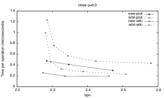
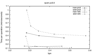
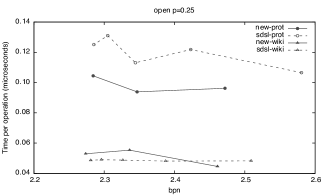
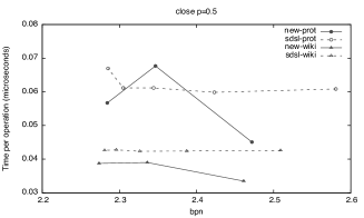
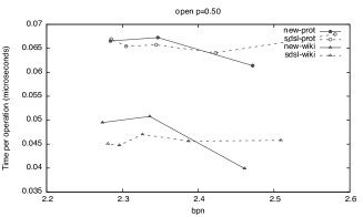
Figure 3: Space-time tradeoffs for our new implementation and the SDSL baseline, for operations $\mathit{close}$ (left) and $\mathit{open}$ (right).

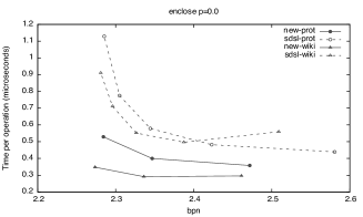
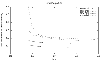
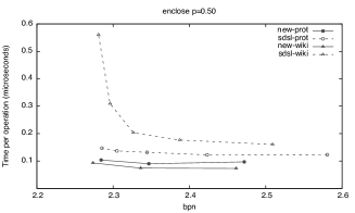
Figure 4: Space-time tradeoffs for our new implementation and the SDSL baseline, for operation $\mathit{enclose}$ (left). On the right, the results as a function of the distance traversed in the parenthesis sequence for $\mathit{rmq}$, $\mathit{close}$, and $\mathit{open}$.

For operation $\mathit{rmq}$ we show the results classified by $j-i$, cut into 100 percentiles. Figure 4 (top right) shows the results. Both structures use the same space, about $2.34$ bits per node. On prot we are significantly faster in almost all the spectrum, while on wiki we are generally faster by a small margin. The difference owes to the fact that the tree of prot is much deeper, and therefore the traversals towards the $\mathit{rmq}$ positions are more random and less cache-friendly. In wiki, the root and the highest nodes are the answers to random $\mathit{rmq}$s in most cases, so their rmM-trees are likely to be in cache from previous queries. On the other hand, we note that the times are basically constant as a function of $j-i$.

The other plots on the right of Figure 4 we show how the times for operation $\mathit{close}$ and $\mathit{open}$ evolve as a function of the difference between the position that is queried and the one where the answer is found. We use the configuration with about $2.34$ bits per node for both implementations, and average the query times over all the tree nodes. In general, only a slight increase is observed as the distance grows. In the larger sequence prot, however, there is a sharp increase for the largest distances. This is not because the number of operations grows sharply, but it rather owes to a 10X increase in the number of cache misses: traversing the longest distances requires accessing various rmM-tree nodes that no longer fit in the cache. Note that the highest times, around 0.5 $\mu$s, are indeed the typical times obtained in Figure 3 with $p=0.0$, where most of the nodes traversed produce cache misses.

5 Conclusions

We have described an alternative solution for representing ordinal trees of $n$ nodes within $2n+\mathcal{O}\!\left(n/\lg n\right)$ bits of space, which solves a large number of queries in time $\mathcal{O}\!\left(\lg\lg n\right)$. While the original solution upon which we build [16] obtains constant times, it is hard to implement and only variants using $\mathcal{O}\!\left(\lg n\right)$ time had been successfully implemented. We have presented a practical implementation of our solution and have experimentally shown that, on real hundred-million node trees, it achieves better space-time tradeoffs than current state-of-the-art implementations. This shows that the new design has not only theoretical, but also practical value. Our new implementation is publicly available at www.dcc.uchile.cl/gnavarro/software.

References

- [1] D. Arroyuelo, R. Cánovas, G. Navarro, and K. Sadakane. Succinct trees in practice. In Proc. 12th Workshop on Algorithm Engineering and Experiments (ALENEX), pages 84–97, 2010.
- [2] M. Bender and M. Farach-Colton. The LCA problem revisited. In Proc. 4th Latin American Theoretical Informatics Symposium (LATIN), LNCS 1776, pages 88–94, 2000.
- [3] M. Bender and M. Farach-Colton. The level ancestor problem simplified. Theoretical Computer Science, 321(1):5–12, 2004.
- [4] D. Benoit, E. D. Demaine, J. I. Munro, R. Raman, V. Raman, and S. S. Rao. Representing trees of higher degree. Algorithmica, 43(4):275–292, 2005.
- [5] Y. T. Chiang, C. C. Lin, and H. I. Lu. Orderly spanning trees with applications. SIAM Journal on Computing, 34(4):924––945, 2005.
- [6] D. Clark. Compact PAT Trees. PhD thesis, University of Waterloo, Canada, 1996.
- [7] M. Fredman and D. Willard. Surpassing the information theoretic bound with fusion trees. Journal of Computer and Systems Science, 47(3):424–436, 1993.
- [8] R. F. Geary, N. Rahman, R. Raman, and V. Raman. A simple optimal representation for balanced parentheses. Theoretical Computer Science, 368(3):231–246, 2006.
- [9] R. F. Geary, R. Raman, and V. Raman. Succinct ordinal trees with level-ancestor queries. ACM Transactions on Algorithms, 2(4):510–534, 2006.
- [10] G. Jacobson. Space-efficient static trees and graphs. In Proc. 30th IEEE Symposium on Foundations of Computer Science (FOCS), pages 549–554, 1989.
- [11] J. Jansson, K. Sadakane, and W.-K. Sung. Ultra-succinct representation of ordered trees with applications. Journal of Computer and System Sciences, 78(2):619–631, 2012.
- [12] S. Joannou and R. Raman. Dynamizing succinct tree representations. In Proc. 11th International Symposium on Experimental Algorithms (SEA), LNCS 7276, pages 224–235, 2012.
- [13] H. Lu and C. Yeh. Balanced parentheses strike back. ACM Transactions on Algorithms, 4(3):1–13, 2008.
- [14] J. I. Munro, R. Raman, V. Raman, and S. S. Rao. Succinct representations of permutations and functions. Theoretical Computer Science, 438:74–88, 2012.
- [15] J. I. Munro and V. Raman. Succinct representation of balanced parentheses and static trees. SIAM Journal on Computing, 31(3):762–776, 2001.
- [16] G. Navarro and K. Sadakane. Fully-functional static and dynamic succinct trees. ACM Transactions on Algorithms, 10(3):article 16, 2014.
- [17] D. Okanohara and K. Sadakane. Practical entropy-compressed rank/select dictionary. In Proc. 9th Workshop on Algorithm Engineering and Experiments (ALENEX), pages 60–70, 2007.
- [18] M. Pătraşcu. Succincter. In Proc. 49th Annual IEEE Symposium on Foundations of Computer Science (FOCS), pages 305–313, 2008.
- [19] H. Yuan and M. J. Atallah. Data structures for range minimum queries in multidimensional arrays. In Proc. 21st Annual ACM-SIAM Symposium on Discrete Algorithms (SODA), pages 150–160, 2010.