Edge-Disjoint Node-Independent Spanning Trees in Dense Gaussian Networks

Abstract

Independent trees are used in building secure and/or fault-tolerant network communication protocols. They have been investigated for different network topologies including tori. Dense Gaussian networks are potential alternatives for 2-dimensional tori. They have similar topological properties; however, they are superiors in carrying communications due to their node-distance distributions and smaller diameters. In this paper, we present constructions of edge-disjoint node-independent spanning trees in dense Gaussian networks. Based on the constructed trees, we design algorithms that could be used in fault-tolerant routing or secure message distribution.

1 Introduction

Parallelism is the performance improvement catalyst in nowadays computing industry. More computing power and higher scalability are being achieved by deploying multi-core processing units [30]. This could vary from multi-core single processing unit in personal computing devices to multi-core multi-processing units on servers and supercomputers. Communications and data exchanges among different processing elements are usually carried on their interconnection network. Thus, an interconnection network is a critical limiting factor on a parallel system overall performance and scalability; consequently, interconnection networks have been receiving considerable research attention for more than forty years [8].

The topology of an interconnection network is a main decisive criterion of its performance qualities. It determines the network communication efficiency as well as its fault tolerance capabilities. There has been plenty of research on interconnection topologies like: arrays, trees, hypercubes, butterfly, meshes, $k$-ary $n$-cubes, and tori [5] [8] [15]. A choice of a topology on which to build a parallel system is constrained by the target performance objectives, contemporary available technology, and simplicity. In the 1960’s arrays and two-dimensional meshes were used to build machines like Illiac [3] and Soloman [24]. Later, hybercubes became popular topologies and machines like Cosmic Cube [22] and nCUBES [19] were built on them. In late 1980’s, meshes, $k$-ary $n$-cube, and toroidal networks started to become more favorable topologies. Cray T3D [20], Cray T3E [21], and Intel Paragon [9] are examples for machines built on these kinds of networks.

An efficient interconnection network called Gaussian network has been introduced in [17]. It is also called a dense Gaussian network [18] when it contains the maximum number of nodes for a given diameter. various facts on some important versions of such networks, defined in a different equivalent way, have been described in [18]. Several related studies on Gaussian networks followed in [10] [23] [26] [36]. Dense Gaussian networks deserve special attention as they are potential alternatives for $N\times N$ tori. They have similar structures, same number of nodes, same number of edges, and both are regular degree four graphs. Dense Gaussian networks, however, possesses smaller diameters and better node-distance distributions. Therefore, they can carry communications more efficiently.

Independent spanning trees can be used in building reliable communication protocols [2][6][7][11] [12][14][25] [27][28][29] [32][34][35]. Given a network $\mathcal{N}$ in which there exist $t$ independent spanning trees rooted in $r$, then $r$ can successfully broadcast a message to every non faulty node $v$ in $\mathcal{N}$ even if up to $t-1$ faulty nodes exist. Since the number of faulty nodes is less than $t$, then at least one of those $t$ node disjoint paths from $r$ to $v$ is fault free. Thus, if $r$ broadcasts through all the existing $t$ independent spanning trees, every non faulty node in $\mathcal{N}$ would receive the broadcasted message. Similarly, if $\mathcal{N}$ has $t$ edge disjoint independent spanning trees, all rooted in $r$, it would be possible to broadcast from $r$ tolerating up to $t-1$ node or edge faults. The communication applications of independent spanning trees are not limited to fault tolerance communication. Independent spanning trees could be utilized in secure message distribution. A message can be split into $t$ packets each of which is sent by $r$ through a different spanning tree to its destination. In this case only the destination would receive all the $t$ packets while every other node would receive at most one of the $t$ packets [16][31][33]. Edge disjoint independent spanning trees can also be used in building efficient casting algorithms. A message of size $M$ can be split into $t$ packets, each of size $M/t$, and simultaneously casted through different trees. Since the trees are edge disjoint, this splitting could result in less packet collisions and higher edge utilization, hence it could reduce the average communication time when wormhole switching is used [1][8].

In this paper, we present a construction of Edge-Disjoint Node-Independent Spanning Trees (EDNIST) in dense Gaussian networks. The rest of the paper is organized as follows. Section 2 introduces some necessary preliminaries. Basic facts on Gaussian networks are briefly summarized in Section 3. Constructions for two edge-disjoint node-independent spanning trees in a dense Gaussian network is described in Section 4. Communication algorithms based on the constructed trees are provided in Section 5. Finally, Section 6 concludes the findings of this paper.

2 Preliminaries

We will denote by $\mathbb{N}=\{0,1,...\}$ the set of all natural numbers and by $\mathbb{Z}=\{\ldots,-2,-1,0,\allowbreak 1,2,\ldots\}$ the set of all integers. An interconnection network is usually modeled as a graph where the computing elements and their wiring are represented as vertices and edges, respectively. An undirected graph is a pair $G=(V,E)$ where $V$ is a set of vertices or nodes, and $E$ is a set of edges . The edges are unordered pairs. We will use the notation $V\left(G\right)=V$, $E\left(G\right)=E$. We are not considering directed graphs in this paper. If $\left(u,v\right)\in E$, we say that $u$ and $v$ are adjacent and that the vertices $u,v$ and the edge $\left(u,v\right)$ are incident with each other. The degree of $v\in V$ is the number of edges in $E$ with which the vertex $v$ is incident. The union of two graphs is defined by $\left(V^{\prime},E^{\prime}\right)\cup$ $\left(V^{\prime\prime},E^{\prime\prime}\right)=\left(V^{\prime}\cup V^{\prime\prime},E^{\prime}\cup E^{\prime\prime}\right)$. A subgraph of a graph $G$ is any graph $G^{\prime}=(V^{\prime},E^{\prime})$ such that $V^{\prime}\subseteq V$ and $E^{\prime}\subseteq E$. Two graphs are vertex-disjoint if their sets of vertices are disjoint. Similarly, two graphs are edge-disjoint if their sets of edges are disjoint. An isomorphism of graphs $G=\left(V,E\right),G^{\prime}=\left(V^{\prime},E^{\prime}\right)$ is a bijection $f:V\rightarrow V^{\prime}$ such that $E^{\prime}=\left\{\left(f\left(u\right),f\left(v\right)\right)|\left(u,v\right)\in E\right\}$; $f$ is an automorphism on $G$ if $G^{\prime}=G$. A path from vertex $u$ to vertex $v$ in $G$ is a sequence $P_{G}\left(u,v\right)=\left(v_{0},v_{1},\ldots,v_{n}\right)$ of pairwise distinct (with the possible exception $v_{0}=v_{n}$) vertices from $V$ such that $u=v_{0}$, $v=v_{n}$, and $\left(v_{i},v_{i+1}\right)\in E$ for $i\in\left\{0,1,\ldots,n-1\right\}$; $n$ is the length of the path $P_{G}\left(u,v\right)$. We will identify the path $\left(v_{0},v_{1},\ldots,v_{n}\right)$ with the subgraph $\left(\left\{v_{0},v_{1},\ldots,v_{n}\right\},\left\{\left(v_{i},v_{i+1}\right)|i\in\left\{0,1,\ldots,n-1\right\}\right\}\right)$. The distance  $d\left(u,v\right)$ between vertices $u,v$ is the length of the shortest path from $u$ to $v$. The diameter of the graph is the maximum distance of two nodes in the graph. A cycle is a path from $u$ to $u$. A graph is connected if, for any $u,v\in V$, there is a path from $u$ to $v$ in $G$. A graph is acyclic if it does not contain a cycle of positive length. A connected acyclic graph is called a tree. In a tree, there is a unique path between any two vertices. A tree is rooted if one of its vertices is denoted as its root. The depth of a rooted tree is the length of the longest path in the tree starting at the root. Given a graph $G=(V,E)$, a spanning tree of $G$ is a subgraph $T=\left(V,E^{\prime}\right)$ being a tree. It is a well-known fact that a connected subgraph $\left(V,E^{\prime}\right)$ of $G$ is a spanning tree if and only if $\left|E^{\prime}\right|=\left|V-1\right|$. Spanning trees have applications in network broadcasting in which a source node sends a message to every other node in the network. A graph may have a number of different spanning trees. Two rooted spanning trees $T_{1},T_{2}$ of $G=\left(V,E\right)$ having the same root $r$ are node independent if, for any vertex $v\in V$, the only common vertices of the paths from $r$ to $v$ in $T_{1}$ and $T_{2}$ are $r$ and $v$.

3 Gaussian Networks

In this paper, we will deal with a special type of graphs called Gaussian networks. The name comes from one possible approach to their definition, based on the subset of complex numbers $\mathbb{Z}\left[\mathbf{i}\right]=\left\{x+y\mathbf{i}|x,y\in\mathbb{Z}\right\}$ with the usual norm $\left\|x+y\mathbf{i}\right\|=x^{2}+y^{2}$. The elements of this set are called Gaussian integers. It is known that for every $\alpha,\beta\in\mathbb{Z}\left[\mathbf{i}\right]$, $\alpha\neq 0$, there exist unique $q,r\in Z[\mathbf{i}]$ such that $\beta=q\alpha+r$ with $\left\|r\right\|<\left\|\alpha\right\|$. In analogue with integers, one can write $\beta\operatorname{mod}\alpha=r$. A Gaussian network $G\left(\alpha\right)=\left(\mathbb{Z}\left[\mathbf{i}\right]_{\alpha},E\left(\alpha\right)\right)$ is given by a fixed Gaussian integer $\alpha\neq 0$. The set of nodes is the residue class modulo $\alpha$. The nodes $\beta$ and $\gamma$ are adjacent if and only if $(\beta-\gamma)\operatorname{mod}\alpha\in\left\{\pm 1,\pm\mathbf{i}\right\}$. Various representations of these residue classes are provided in [13]. Gaussian networks are regular. The degree of each vertex is four. They are highly symmetric; in fact they are vertex-transitive. For every pair $u,v\in\mathbb{Z}\left[\mathbf{i}\right]_{\alpha},$ there is an automorphism of $G\left(\alpha\right)$ mapping $u$ to $v$. The total number of nodes in the network $G\left(\alpha\right)$ is $\left\|\alpha\right\|$. The distance distribution for Gaussian networks can be found in [17] where the diameter of the network $G\left(x+y\mathbf{i}\right)$ is equal to $y$ if $\left\|x+y\mathbf{i}\right\|$ is even and to $y-1$ otherwise. Gaussian networks are closely related to circulant graphs. A circulant graph with $N\geq 1$ vertices and two jumps $a,b$, where $1\leq a<b$ is the graph $C_{N}\left(a,b\right)$ where $V(C_{N}(a,b))=\left\{0,1,\ldots,N-1\right\}$ and, for $u,v\in V$, $\left(u,v\right)\in E(C_{N}(a,b))$ if $\left|u-v\right|\operatorname{mod}N\in\left\{a,b,N-a,N-b\right\}$. $C_{a^{2}+b^{2}}\left(a,b\right)$ is isomorphic to $G(a+bi)$ if and only if $\gcd\left(a,b\right)=1$ [17]. A Gaussian network is dense when it has a maximum number of nodes for a given diameter $k$. It is shown in [4] that this is the case in the graph $C_{k^{2}+\left(k+1\right)^{2}}\left(k,k+1\right)$. In this paper, we deal with these dense diameter-optimal graph, which is isomorphic to the Gaussian network $G\left(\alpha_{k}\right)$, where $\alpha_{k}=k+\left(k+1\right)\mathbf{i}$, since $\gcd(k,k+1)=1$. We denote $G_{k}=\left(V_{k},E_{k}\right)=G\left(\alpha_{k}\right)$, $k\geq 1$. We will call an edge in $G_{k}$ to be horizontal if it is of the form $\left(u,\left(u\pm 1\right)\operatorname{mod}\alpha_{k}\right)$ and vertical if it is of the form $\left(u,\left(u\pm\mathbf{i}\right)\operatorname{mod}\alpha_{k}\right)$. A path in $G_{k}$ is horizontal (vertical) if does not contain a vertical (horizontal) edge. We depict the graph $G_{k}$ the usual way the complex numbers are depicted in the Cartesian plane. The vertex $a+b\mathbf{i}$, $\left|a\right|+\left|b\right|\leq k$, will be positioned at point $\left\langle a,b\right\rangle$. The graph $G_{3}$ is depicted in Fig. 1.

Figure 1: Gaussian network generated with $\alpha=3+4i$.

4 Edge-disjoint node-independent spanning trees in Gaussian networks

We will present here a solution to the problem of finding a set of edge-disjoint node-independent spanning trees in the Gaussian network $G_{k}$.

Proposition 1

Let $\mathcal{T}_{k}$ be a set of edge-disjoint spanning trees in $G_{k}$, then $\left|\mathcal{T}_{k}\right|\leq~{}2$.

Proof:

The total number of nodes in $G_{k}=2k^{2}+2k+1$. Hence, each spanning tree in $\mathcal{T}_{k}$ must have exactly $2k^{2}+2k$ edges. Since the total number of edges in $G_{k}=4k^{2}+4k+2$, and the trees in $\mathcal{T}_{k}$ are edge disjoint, it follows that $\left|\mathcal{T}_{k}\right|\leq 2$. ∎

In our further considerations, we will use automorphisms $\rho$ and $\sigma$ of the Gaussian network $G_{k}$, $k\geq 2$. The mapping $\rho$ is the $90^{\circ}$ counterclockwise rotation. It is defined, for $a+b\mathbf{i}\in V_{k}$, by $\rho\left(a+b\mathbf{i}\right)=\mathbf{i}\left(a+b\mathbf{i}\right)=-b+a\mathbf{i}$. The mapping $\sigma$ is the symmetry with respect to the axis of the second and the fourth quadrants. It is defined, for $a+b\mathbf{i}\in V_{k}$, by $\sigma\left(a+b\mathbf{i}\right)=-b-a\mathbf{i}$. The mappings satisfy the relations $\rho^{2}\sigma=\sigma\rho^{2}$ and $\rho^{4}=\sigma^{2}=\mathbf{1}$, where $\mathbf{1}$ is the identity mapping. Each of $\rho$ and $\sigma$ maps a horizontal edge to a vertical one and vice versa. We will now describe two subgraphs of $G_{k}$: the “black subgraph” $B_{k}$, and the “red subgraph” $R_{k}$, being our candidates for the two edge-disjoint node-independent spanning trees. Each of $B_{k}$ and $R_{k}$ is the union of several component subgraphs of $G_{k}$. These components will be obtained by applying the mappings $\rho$ and $\sigma$ to the following graphs:

1. The array subgraph $A$:
$V\left(A\right)=\left\{a+b\mathbf{i|}0\leq a\leq k-1,1\leq b\leq k,a+b\leq k\right\},$
$E\left(A\right)=\left\{\left(a+b\mathbf{i},\left(a+1\right)+b\mathbf{i}\right)|0\leq a\leq k-2,1\leq b\leq k-1,a+b\leq k-1\right\}$; $A$ contains all possible horizontal edges among $V(A)$.
The edge size of $A\$is $\left|E\left(A\right)\right|=k\left(k-1\right)/2$.

2. The baseline subgraph $B$:
$V\left(B\right)=\left\{a\mathbf{|}0\leq a\leq k\right\},$
$E\left(B\right)=\left\{\left(a,\left(a+1\right)\right)|0\leq a\leq k-1\right\}$; $B$ contains all possible horizontal edges among $V(B)$.
The edge size of $B\$is $\left|E\left(B\right)\right|=k$.

3. The $\ B_{k}$-specific wrap-around graph $W^{B}$:
$V\left(W^{B}\right)=\left\{a+b\mathbf{i}|,\left|a+b\right|=k\text{, and }0\leq a,1\leq b\text{ or }a\leq 0,b\leq-1\right\},$
$E\left(W^{B}\right)=\left\{\left(a+b\mathbf{i},-\left(b-1\right)+\left(-1-a\right)\mathbf{i}\right)|a+b=k,0\leq a,1\leq b\right\}$; $W^{B}$ contains all possible horizontal edges among $V(W^{B})$.
The edge size of $W^{B}\$is $\left|E\left(W^{B}\right)\right|=k$.

4. The $\ R_{k}$-specific wrap-around graph $W^{R}$:
$V\left(W^{R}\right)=\left\{a+b\mathbf{i}|1\leq a,b\leq 0\text{ or }a\leq 0,b\geq 1\text{, and }\left|a+b\right|=k\right\},$
$E\left(W^{R}\right)=\left\{\left(a+b\mathbf{i},b+a\mathbf{i}\right)|a-b=k,1\leq a,b\leq 0\right\}$; $W^{R}$ contains all possible horizontal edges among $V(W^{R})$
The edge size of $W^{R}\ \left|E\left(W^{R}\right)\right|=k$.

The subgraph $B_{k}$ is defined as:

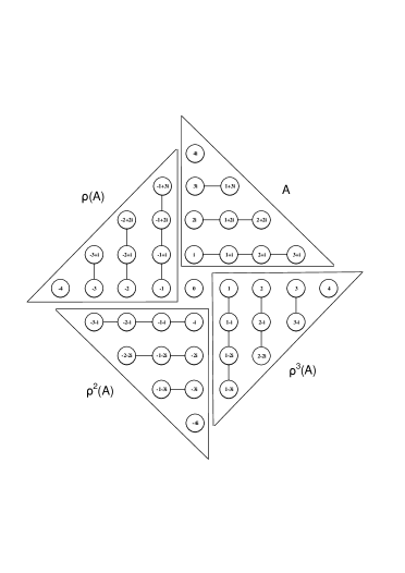
(a) Array graphs

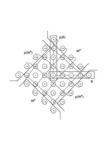
(b) Baseline and $B_{4}$-specific wrap-around graphs

Figure 2: $B_{4}$ components ($k=4$)

$$B_{k}=A\cup\rho\left(A\right)\cup\rho^{2}\left(A\right)\cup\rho^{3}\left(A\right)\cup B\cup\rho\left(B\right)\cup W^{B}\cup\rho\left(W^{B}\right)$$ (1)

Fig. 2 depicts the components of $B_{4}$.

The subgraph $R_{k}$ is defined as:

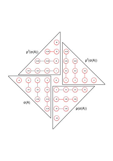
(a) Array graphs

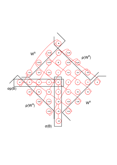
(b) Baseline and $R_{4}$-specific wrap-around graphs

Figure 3: $R_{4}$ components ($k=4$)

$$R_{k}=\sigma\left(A\right)\cup\rho\sigma\left(A\right)\cup\rho^{2}\sigma\left(A\right)\cup\rho^{3}\sigma\left(A\right)\cup\sigma\left(B\right)\cup\sigma\rho\left(B\right)\cup W^{R}\cup\rho\left(W^{R}\right)$$ (2)

Fig. 3 shows the components of $R_{4}$, and Fig. 4 limns $B_{4}$ and $R_{4}$.

Proposition 2

$B_{k}$ and $R_{k}$ have the following basic properties:
1. The vertex set of each of the graphs $B_{k}$ and $R_{k}$ is $V_{k}$.
2. The edge sets of all components of $B_{k}$, as stated in $(\ref{BU})$ are pairwise disjoint. The edge sets of all components of $R_{k}$, as stated in $(\ref{RU})$ are pairwise disjoint.
3. Each of the graphs $B_{k}$ and $R_{k}$ consists of $2k^{2}+2k$ edges.
4. The edge sets of $B_{k}$ and $R_{k}$ are disjoint.

Proof:

1. The following can be observed from the construction of the subgraphs $B_{k}$ and $R_{k}$:

$$V_{k} =V\left(A\right)\cup V\left(\rho\left(A\right)\right)\cup V\left(\rho^{2}\left(A\right)\right)\cup V\left(\rho^{3}\left(A\right)\right)\cup V\left(B\right)$$

$$V_{k} =V\left(\sigma\left(A\right)\right)\cup V\left(\rho\sigma\left(A\right)\right)\cup V\left(\rho^{2}\sigma\left(A\right)\right)\cup V\left(\rho^{3}\sigma\left(A\right)\right)\cup V\left(\sigma\left(B\right)\right)$$

2. Let $C_{1},C_{2}$ be two distinct components of $B_{k}$. If $C_{1},C_{2}$ are not node-disjoint then all edges in one of these components are horizontal and all edges in the other one are vertical. A similar argument is valid for $R_{k}$.

3. Since the components of $B_{k}$ are edge-disjoint, the edge-size of $B_{k}$ is the sum of the edge-sizes of the components. The mappings $\rho,\sigma$ preserve the edge-size of a graph. The same argument applies to $R_{k}$. Therefore, a summation of the edge-disjoint component sizes yields:

$$\left|E\left(B_{k}\right)\right| =4\left|E\left(A\right)\right|+2\left|E\left(B\right)\right|+2\left|E\left(W^{B}\right)\right|$$

$$=4\Big{[}\frac{k\left(k-1\right)}{2}\Big{]}+2k+2k=2k^{2}+2k$$

$$\left|E\left(R_{k}\right)\right| =4\left|E\left(A\right)\right|+2\left|E\left(B\right)\right|+2\left|E\left(W^{R}\right)\right|$$

$$=4\Big{[}\frac{k\left(k-1\right)}{2}\Big{]}+2k+2k=2k^{2}+2k\text{.}$$

4. Comparing any component of $B_{k}$ to any component of $R_{k}$, one can observe that such pair of components either does not contain a common pair of vertices or the direction of the edges in the two components are different. Hence, $B_{k}$ and $R_{k}$ are edge-disjoint. ∎

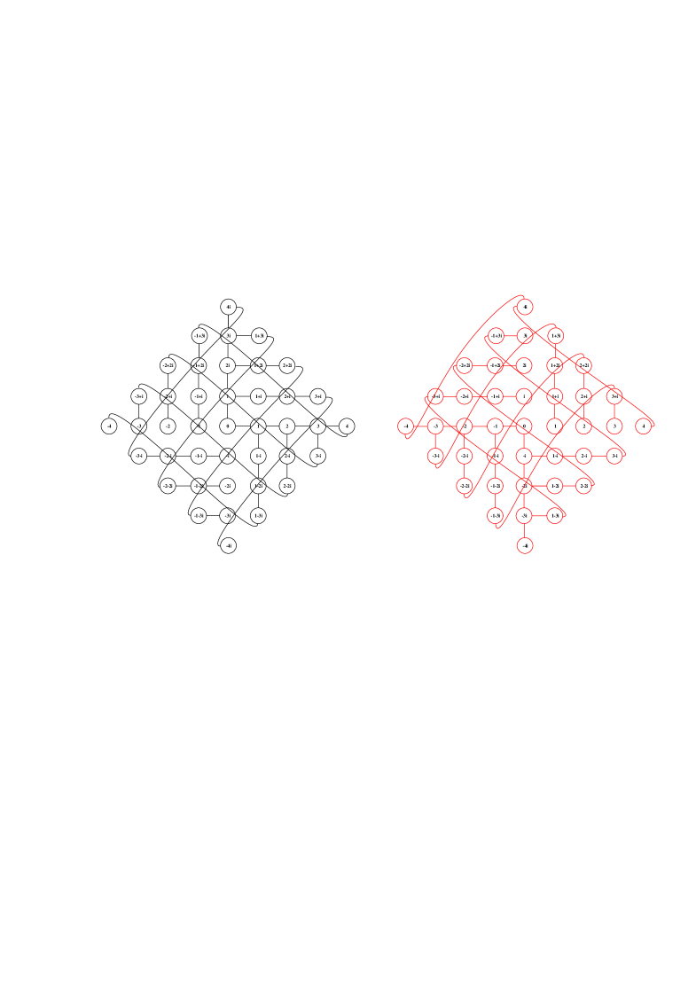
Figure 4: The trees $B_{4}$ and $R_{4}$

Lemma 3

Each of the graphs $B_{k}$ and $R_{k}$ is a connected graph.

Proof:

First, we will show that $B_{k}$ is connected. $B$ is connected by construction. $\rho(B)$ is a rotation of B, and hence, it is connected. $B\cup\rho(B)$ is connected since $B\cap\rho(B)=\left\{0\right\}\neq\phi$. There exist paths between: every node in $A$ and some node in $\rho(B)\subset A$, every node in $\rho^{3}(A)$ and some node in $B\subset\rho^{3}(A)$, every node in $\rho(A)$ and some node in $\rho^{3}(A)$ through $\rho(W^{B})$, and every node in $\rho^{2}(A)$ and some node in $A$ through $W^{B}$. Thus, $B_{k}$ is connected. A similar argument can be used to show that $R_{k}$ is connected. ∎

Corollary 4

$B_{k}$ and $R_{k}$ are edge-disjoint spanning trees in $G_{k}$.

Proof:

Following Lemma 3 and Proposition 2, $B_{k}$ and $R_{k}$ are connected, edge-disjoint, and the edge size of each of them is $\left|V_{k}\right|-1$. Therefore, they are edge-disjoint spanning trees in $G_{k}$. ∎

In the remaining text we will assume that the spanning trees $B_{k}$ and $R_{k}$ are rooted at node $0$. The following three lemmata will be useful in proving our main result expounded in Theorem 8 and Theorem 11.

Let $H^{B}=A\cup W^{B}\cup\rho^{2}\left(A\right)$, and $H^{R}=\rho\sigma\left(A\right)\cup W^{R}\cup\rho^{3}\sigma\left(A\right)$.

Lemma 5

Each path in $H^{B}$ or in $H^{R}$ is horizontal and not longer than $k$ or $(k+1)$, respectively.

Proof:

The paths being horizontal or vertical follow from the definition of the sets $A,B$ and $W^{B},W^{R}$. Each path in $A$ or $\rho^{2}\left(A\right)$ is of some length $i$, $i\in\left\{0,\ldots,k-1\right\}$. Any path in $W^{B}$ is of length one. A path of length $i$ in $A$ is connected by an edge in $W^{B}$ to a single path in $\rho^{2}\left(A\right)$ of length $k-i-1$. The maximum length of a path in $H^{B}$ is therefore $i+1+\left(k-i-1\right)=k$. Fig. 5 illustrates $H^{B}$ paths when $k=4$.

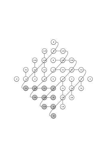
(a) $W^{B}$ wrapped-around edges

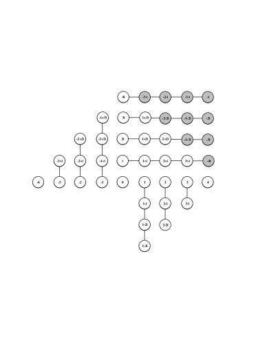
(b) $W^{B}$ straightened edges

Figure 5: $H^{B}$ paths in $B_{4}$

Each path in $\rho\sigma\left(A\right)$ or in $\rho^{3}\sigma\left(A\right)$ is of some length $i$, $i\in\left\{0,\ldots,k-1\right\}$. Any path in $W^{R}$ is of length one. A path of length $i$ in $\rho\sigma\left(A\right)$ is connected by an edge in $W^{R}$ to a single path in $\rho^{3}\sigma\left(A\right)$ of length $k-i$. The maximum length of a path in $H^{B}$ is therefore $i+1+\left(k-i\right)=k+1$. Fig. 6 illustrates $H^{R}$ paths when $k=4$.

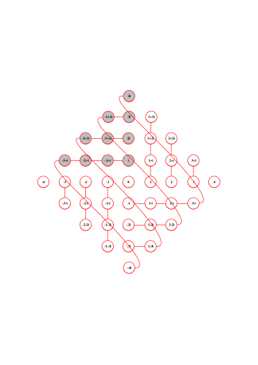
(a) $W^{R}$ wrapped-araound edges

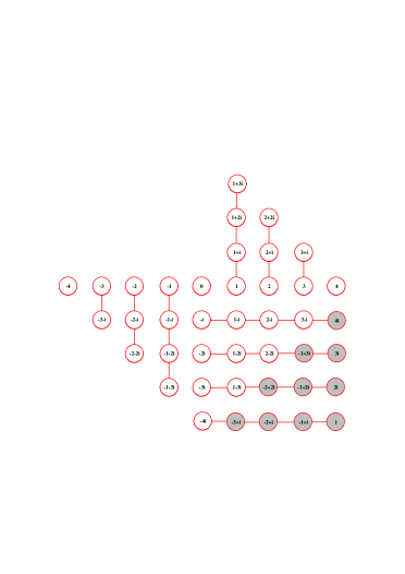
(b) $W^{R}$ straightened edges

Figure 6: $H^{R}$ paths in $R_{4}$

∎

Lemma 6

The longest path in $B_{k}$ or in $R_{k}$ starting at node $0$ is of length $2k$, $k\geq 2$.

Proof:

It is useful to observe that the properties of the mapping $\rho$ and Lemma 5 imply that the length of a path is at most $k$ in $\rho\left(H^{B}\right)$ and at most $(k+1)$ in $\rho\left(H^{R}\right)$.
The longest path in $\rho\left(B\right)$ is of length $k$. Any path in $B_{k}$ starting at node $0$ having an initial segment in $\rho\left(B\right)$ may continue through $H^{B}$ only. Following Lemma 5, the length of such path is at most $k+k=2k$. This may happen only if the initial segment is of length $k$ and, consequently, the path leads to node $-\mathbf{i}$.
Similar reasoning applies to $B$ and $\rho\left(H^{B}\right)$. Any path in $B_{k}$ starting at node $0$ having an initial segment in $B$ may continue through $\rho\left(H^{B}\right)$ only. The longest path of this kind is, therefore, of length $2k$ and leads to node $-1$.
The longest path in $\sigma\left(B\right)$ starting at node $0$ is of length $k$ and cannot be extended. Any other path in $\sigma\left(B\right)$ is of length $k-1$ or less. Any path in $R_{k}$ starting at node $0$ having an initial segment in $\sigma\left(B\right)$ may continue through $H^{R}$ only. Following Lemma 5, the length of such path is at most $\left(k-1\right)+\left(k+1\right)=2k$. This may happen only if the initial segment is of length $(k-1)$, and thus, the path leads to node $\mathbf{i}$.
The longest path in $\sigma\rho\left(B\right)$ starting at node $0$ is of length $k$ and may continue in $R_{k}$ by a path of length two or less. The total length is then not larger than $k+2\leq 2k$, since $k\geq 2$; the equality takes place for a path leading to node $k$ only if $k=2$. Any path in $R_{k}$ starting at node $0$ having an initial segment shorter than $k$ in $\sigma\rho\left(B\right)$ may continue through $\rho\left(H^{R}\right)$ only. Accordingly, The longest path of this kind is of length $\left(k-1\right)+\left(k+1\right)=2k$. This may happen only if the initial segment is of length $k-1$, and hence, the path leads to node $1$. ∎

Lemma 7

A horizontal path and a vertical path in $G_{k}$, each being of length $k+1$ or less, can have at most two common nodes. This may happen only if one of the paths is of length $k+1$ and the two common nodes are its starting and ending nodes.

Proof:

Assume a horizontal and a vertical paths, each being of length $k+1$ or less, having at least one node in common. Since $G_{k}$ is vertex-transitive, we can assume, without loss of generality, that the common node is $0$. The paths initial segments of size $k$ starting from $0$ are line segments and cannot intersect in more than one node. Therefore, another common node may exist only if one of the paths is of length $k+1$ and $0$ is its starting node, the last edge of such path is a wrap-around edge, and the other common node is the ending node of the path. ∎

Theorem 8

$B_{k}$ and $R_{k}$ are edge-disjoint node-independent spanning trees in $G_{k}$ each of depth $2k$, $k\geq 2$.

Proof:

Let $k\geq 2$. Then $B_{k}$ and $R_{k}$ are edge-disjoint spanning trees in $G_{k}$ by Corollary 4. Since both trees are rooted in $0$ and following Lemma 6, the depth of each tree is $2k$. To complete the proof of this theorem, we need to prove that $B_{k}$ and $R_{k}$ are node independent. Let $v\in V_{k}$. Assume, in contrary, a node $u$ being an intermediate node of both: the path from $0$ to $v$ in $B_{k}$, and the path from $0$ to $v$ in $R_{k}$. Then $u$ is of degree two in both trees. The node $v$ cannot belong to $V\left(X\right)$, where $X=B\cup\rho(B)\cup\sigma(B)\cup\sigma\rho(B)$, since otherwise in one of the trees the path to $v$ leads exclusively through nodes of degree three. Let $v\in V\left(G_{k}\right)-V(X)$. The path from $0$ to $v$ starts in both trees by a segment in $X$ and then continues by a segment in one of $H^{B},H^{R},\rho\left(H^{B}\right),\rho\left(H^{R}\right)$. The node $u$ cannot belong to $V\left(X\right)$, since the only such $u$ being of degree two in both trees is $u=k\mathbf{i}$; the only path in $R_{k}$ with intermediate node $k\mathbf{i}$ leads to node $k$, while the path to $k$ in $B_{k}$ does not contain $k\mathbf{i}$. Hence, $u$ belongs to one of $H^{B}\cap\rho\left(H^{R}\right)$ or $\rho\left(H^{B}\right)\cap H^{R}$. It follows by Lemma 5 and the $\rho$ mapping that $u$ belongs to an intersection of a horizontal and a vertical paths, each being of length $k+1$ or less. Lemma 7 implies that one of these paths is of length $(k+1)$ and its starting and ending nodes are $u$ and $v$. This leads to a contradiction since such a path may exist only if $u,v\in V(X)$. ∎

Remark 9

The only two edges in $E_{k}$ not belonging to the graphs $B_{k}$ or $R_{k}$ are the edges $\left(-k,-k\mathbf{i}\right)$ and $\left(k,-k\mathbf{i}\right)$.

$B_{1}$ and $R_{1}$ are depicted in Fig. 7. As it can be seen, $B_{1}$ is of depth two; however, $R_{1}$ is of depth three. We can define $R^{\prime}_{k}=(V(R_{k}),E(R_{k})-\{(k,i)\}+\{(k,-i)\})$. $R^{\prime}_{1}$ is illustrated in Fig. 7(c), and its depth is clearly two.

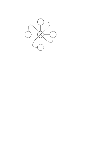
(a) $B_{1}$

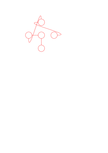
(b) $R_{1}$

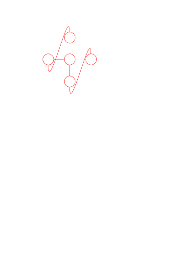
(c) $R^{\prime}_{1}$

Figure 7: $B_{1}$, $R_{1}$, and $R^{\prime}_{1}$

Remark 10

The path $P_{R^{\prime}_{k}}(0,k)$ is shorter than $P_{R_{k}}(0,k)$ by one, and the only two edges in $E_{k}$ not belonging to the graphs $B_{k}$ or $R^{\prime}_{k}$ are $\left(-k,-k\mathbf{i}\right)$ and $\left(k,k\mathbf{i}\right)$.

Theorem 11 below extends Theorem 8 to prove that $B_{k}$ and $R^{\prime}_{k}$ are edge-disjoint node-independent spanning trees in $G_{k}$, $k\geq 1$.

Theorem 11

$B_{k}$ and $R^{\prime}_{k}$ are edge-disjoint node-independent spanning trees in $G_{k}$ each of depth $2k$, $k\geq 1$.

Proof:

By Theorem 8, $B_{k}$ and $R_{k}$ are edge-disjoint node-independent spanning trees in $G_{k}$, $k\geq 2$. Disconnecting a leaf node from $R_{k}$ and reconnecting it to another node results again in a connected graph. This implies that $R^{\prime}_{k}$ is a spanning tree in $G_{k}$.
Only one edge in $R^{\prime}_{k}$ does not belong to $R_{k}$, and this edge is unused in $B_{k}$. Thus, $B_{k}$ and $R^{\prime}_{k}$ are edge-disjoint spanning trees in $G_{k}$.
All paths in $R^{\prime}_{k}$ are identical to those in $R_{k}$ except for the path that leads to $k$. To prove that $B_{k}$ and $R^{\prime}_{k}$ are node-independent spanning trees, we only need to verify that the paths lead to $k$ in $B_{k}$ and in $R^{\prime}_{k}$ are node-disjoint. In $B_{k}$, the path form $0$ to $k$ leads exclusively through nodes of degree three. These nodes must be leaves in $R^{\prime}_{k}$ and cannot be intermediate nodes in any path. Hence, $B_{k}$ and $R^{\prime}_{k}$ are edge-disjoint node-independent spanning trees in $G_{k}$, $k\geq 2$.
The distance from $0$ to $k$ in $R^{\prime}_{k}$ equals the distance from $0$ to $-k\mathbf{i}$ plus one = $k+1<2k$, $k\geq 2$. Therefore, $B_{k}$ and $R^{\prime}_{k}$ are of depth $2k$, $k\geq 2$.
The theorem can be easily verified for $k=1$, and this concludes the theorem proof. ∎

$B_{4}$ and $R^{\prime}_{4}$ are depicted in Fig. 8.

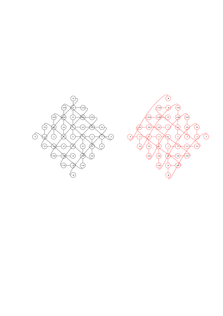
Figure 8: The trees $B_{4}$ and $R^{\prime}_{4}$

5 Routing in $G_{k}$ using edge-disjoint node-independent trees

The existence of two edge-disjoint node-independent spanning trees in $G_{k}$ makes it possible to tolerate either one node or one edge failure. Sending a message along both trees guarantees the message delivery in case of a single failure of either a node or an edge. The trees also can be utilized to securely distribute a message by splitting it into two packages each of which is sent to the destination along a different tree. Since the trees are node independents, the paths to the destinations in those trees are disjoint. This guarantees that only the destination will receive all the packages. Note that in both of the above applications the communications must be initiated from the root. However, it is possible for each node $v$ to implicitly construct two edge-disjoint node-independent spanning trees rooted in $v$ itself.

We present routing algorithms for such usage when the source node $s_{1}+s_{2}\mathbf{i}$ sends a message to a destination node $d_{1}+d_{2}\mathbf{i}$ along $B_{k}$ or $R^{\prime}_{k}$, $k\geq 1$. The algorithms are based on the vertex-transitive property of $G_{k}$. The source node is mapped to node $0$. The destination node and every transient node are mapped accordingly. Algorithm 1 outlines the routing in the source node. The tree type and the destination mapped location determine the message direction from the source node. Table I summarizes all possible directions form the source node and the exclusive condition associated with each direction.

Algorithm 2 describes the routing in a non-source node. If a receiving node is the destination, then no further routing is required. Otherwise the receiving node is a transient node and the message is rerouted after deciding its new direction. By default, a message keeps flowing in the same direction unless it needs to make a turn. A message makes a turn only if the transient node lays on the horizontal axis or the vertical axis, and the destination lays on a continuing path in $H^{B}$ or $H^{R}$. Table II shows the two exclusive possible conditions in which a message needs to make a turn, and it associates each condition with the message new direction. If non of these conditions holds, then the default case applies.

Algorithm 1 Routing algorithm for a source node $s_{1}+s_{2}\mathbf{i}$ to send a message to a destination node $d_{1}+d_{2}\mathbf{i}$ through $B_{k}$ or $R^{\prime}_{k}$

1:  Compute the mapped location of the destination:      $d_{1}^{m}+d_{2}^{m}\mathbf{i=}\left(\left(d_{1}+d_{2}\mathbf{i}\right)-\left(s_{1}+s_{2}\mathbf{i}\right)\right)\operatorname{mod}\alpha_{k}$

2:  Use Table I to determine the message direction Dir

3:  Create the message header: $\left(\left\langle s_{1},s_{2}\right\rangle,\left\langle d_{1}^{m},d_{2}^{m}\right\rangle,\textbf{Dir}\right)$ and send the message

Algorithm 2 Routing algorithm for a non-source node $t_{1}+t_{2}\mathbf{i}$

1:  Read the message header $\left(\left\langle s_{1},s_{2}\right\rangle,\left\langle d_{1}^{m},d_{2}^{m}\right\rangle,\textbf{Dir}\right)$

2:  Compute the current node mapped location:      $t_{1}^{m}+t_{2}^{m}\mathbf{i=}\left(\left(t_{1}+t_{2}\mathbf{i}\right)-\left(s_{1}+s_{2}\mathbf{i}\right)\right)\operatorname{mod}\alpha_{k}$

3:  if $\left\langle d_{1}^{m},d_{2}^{m}\right\rangle=\left\langle t_{1}^{m},t_{2}^{m}\right\rangle$ then

4:     Accept the message and exit

5:  else

6:     Use Table II to decide the message direction NewDir

7:     Create the new message header: $\left(\left\langle s_{1},s_{2}\right\rangle,\left\langle d_{1}^{m},d_{2}^{m}\right\rangle,\textbf{NewDir}\right)$ and send the message

8:  end if

Condition	$B_{k}$ Direction	$R^{\prime}_{k}$ Direction	$d_{1}^{m}+d_{2}^{m}\mathbf{i}$ Location
$d_{1}^{m}\times d_{2}^{m}>0$	$+\mathbf{i}$	$-1$	Quadrant 1 or 3
$d_{1}^{m}\times d_{2}^{m}<0$	$+1$	$-\mathbf{i}$	Quadrant 2 or 4
$d_{2}^{m}=0$	$+1$	$-1$	Horizontal Axis
$d_{1}^{m}=0$	$+\mathbf{i}$	$-\mathbf{i}$	Vertical Axis

TABLE I: The source node routing table

Condition	NewDir	Location
		$t_{1}^{m}+t_{2}^{m}\mathbf{i}$	$d_{1}^{m}+d_{2}^{m}\mathbf{i}$
			$B_{k}$	$R^{\prime}_{k}$
$(t_{2}^{m}=0)$ AND		On Horizontal Axis	Quadrant 2 or 4	Quadrant 1 or 3
$(t_{1}^{m}=d_{1}^{m}$ OR $t_{1}^{m}=d_{1}^{m}+k+1$ OR $t_{1}^{m}=d_{1}^{m}-k)$	$-\mathbf{i}$
$\left(t_{1}^{m}=0\right)$ AND		On Vertical Axis	Quadrant 1 or 3	Quadrant 2 or 4
$(t_{2}^{m}=d_{2}^{m}$ OR $t_{2}^{m}=d_{2}^{m}+k+1$ OR $t_{2}^{m}=d_{2}^{m}-k)$	$+1$
Default	Dir	Keep the message flowing in the same direction.

TABLE II: A transient node routing table

6 Conclusions

We introduced two constructions of edge-disjoint node-independent spanning trees in dense Gaussian networks. By taking advantage of the node-transitivity in dense Gaussian networks, we defined a limited number of subgraphs and deployed a rotation technique to construct the first pair of trees. The depth of each tree in the first construction is $2k$, $k\geq 2$, where $k$ is the network diameter. We extended the first construction to construct the second pair of trees. The depth of each tree in the second construction is $2k$, $k\geq 1$. Based on the second construction, we designed algorithms that can be used in fault-tolerant routing or secure message distribution. The source node in these algorithms is not restricted to a specific node; it could be any node in $G_{k}$.

In our future work we intend to investigate constructing independent spanning trees and completely independent spanning trees in dense Gaussian networks. Our initial investigations indicate that applying similar techniques to those deployed in this paper could lead to fruitful outcomes.

References

- [1] O. Alsaleh, B. Bose, and B. Hamdaoui, “One-to-many node-disjoint paths routing in dense gaussian networks,” The Computer Journal, vol. 58, no. 2, pp. 173–187, 2015.
- [2] F. Bao, Y. Igarashi, and S. R. Öhring, “Reliable broadcasting in product networks,” Discrete Applied Mathematics, vol. 83, no. 1-3, pp. 3–20, 1998.
- [3] G. H. Barnes, R. M. Brown, M. Kato, D. J. Kuck, D. L. Slotnick, and R. Stokes, “The ILLIAC IV computer,” IEEE Trans. Comput., vol. C-17, no. 8, pp. 746–757, 1968.
- [4] R. Beivide, E. Herrada, J. L. Balcázar, and A. Arruabarrena, “Optimal distance networks of low degree for parallel computers,” IEEE Trans. Comput., vol. 40, no. 10, pp. 1109–1124, 1991.
- [5] B. Bose, B. Broeg, Y. Kwon, and Y. Ashir, “Lee distance and topological properties of k-ary n-cubes,” Computers, IEEE Transactions on, vol. 44, no. 8, pp. 1021–1030, 1995.
- [6] Y.-H. Chang, J.-S. Yang, J.-M. Chang, and Y.-L. Wang, “A fast parallel algorithm for constructing independent spanning trees on parity cubes,” Applied Mathematics and Computation, vol. 268, pp. 489 – 495, 2015.
- [7] B. Cheng, J. Fan, and X. Jia, “Dimensional-permutation-based independent spanning trees in bijective connection networks,” Parallel and Distributed Systems, IEEE Transactions on, vol. 26, no. 1, pp. 45–53, 2015.
- [8] W. J. Dally and B. P. Towles, Principles and practices of interconnection networks. Elsevier, 2004.
- [9] R. Esser and R. Knecht, Intel Paragon XP/S-Architecture and software environment. Springer, 1993.
- [10] M. Flahive and B. Bose, “The topology of Gaussian and Eisenstein-Jacobi interconnection networks,” IEEE Trans. Parallel Distrib. Syst., vol. 21, no. 8, pp. 1132–1142, Aug. 2010.
- [11] P. Fragopoulou and S. G. Akl, “Edge-disjoint spanning trees on the star network with applications to fault tolerance,” IEEE Trans. Computers, vol. 45, no. 2, pp. 174–185, 1996.
- [12] A. Itai and M. Rodeh, “The multi-tree approach to reliability in distributed networks,” Information and Computation, vol. 79, no. 1, pp. 43–59, 1988.
- [13] J. Jordan and C. Potratz, “Complete residue systems in the Gaussian integers,” Mathematics Magazine, vol. 38, no. 1, pp. 1–12, 1965.
- [14] L. Kong, M. Ali, and J. S. Deogun, “Building redundant multicast trees for preplanned recovery in WDM optical networks,” J. High Speed Netw., vol. 15, no. 4, pp. 379–398, Oct. 2006.
- [15] F. T. Leighton, Introduction to parallel algorithms and architectures: Arrays· trees· hypercubes. Morgan Kauffman, 1992.
- [16] J.-C. Lin, J.-S. Yang, C.-C. Hsu, and J.-M. Chang, “Independent spanning trees vs. edge-disjoint spanning trees in locally twisted cubes,” Information Processing Letters, vol. 110, no. 10, pp. 414 – 419, 2010.
- [17] C. Martinez, R. Beivide, E. Stafford, M. Moreto, and E. M. Gabidulin, “Modeling toroidal networks with the Gaussian integers,” IEEE Transactions on Computers, vol. 57, no. 8, pp. 1046–1056, 2008.
- [18] C. Martínez, E. Vallejo, R. Beivide, C. Izu, and M. Moretó, “Dense Gaussian networks: suitable topologies for on-chip multiprocessors,” International Journal of Parallel Programming, vol. 34, no. 3, pp. 193–211, 2006.
- [19] C. Ncube, “The ncube family of high-performance parallel computer systems,” in Proceedings of the Third Conference on Hypercube Concurrent Computers and Applications: Architecture, Software, Computer Systems, and General Issues - Volume 1, ser. C3P. New York, NY, USA: ACM, 1988, pp. 847–851.
- [20] I. C. Research, “Cray T3D system architecture overview manual.”
- [21] S. L. Scott et al., “The cray T3E network: adaptive routing in a high performance 3D torus,” 1996.
- [22] C. L. Seitz, “The cosmic cube,” Communications of the ACM, vol. 28, no. 1, pp. 22–33, 1985.
- [23] A. Shamaei, B. Bose, and M. Flahive, “Higher dimensional Gaussian networks,” in Proceedings of the 2014 IEEE International Parallel & Distributed Processing Symposium Workshops, ser. IPDPSW ’14. Washington, DC, USA: IEEE Computer Society, 2014, pp. 1438–1447.
- [24] D. L. Slotnick, W. C. Borck, and R. C. McReynolds, “The solomon computer,” in Proceedings of the December 4-6, 1962, Fall Joint Computer Conference, ser. AFIPS ’62 (Fall). New York, NY, USA: ACM, 1962, pp. 97–107.
- [25] A. Touzene, “Edges-disjoint spanning trees on the binary wrapped butterfly network with applications to fault tolerance,” Parallel Comput., vol. 28, no. 4, pp. 649–666, Apr. 2002.
- [26] ——, “On all-to-all broadcast in dense Gaussian network on-chip,” Parallel and Distributed Systems, IEEE Transactions on, vol. 26, no. 4, pp. 1085–1095, 2015.
- [27] A. Touzene, K. Day, and B. Monien, “Edge-disjoint spanning trees for the generalized butterfly networks and their applications,” J. Parallel Distrib. Comput., vol. 65, no. 11, pp. 1384–1396, 2005.
- [28] Y.-C. Tseng, S. yuan Wang, and C.-W. Ho, “Efficient broadcasting in wormhole-routed multicomputers: A network-partitioning approach,” IEEE Transactions on Parallel and Distributed Systems, vol. 10, pp. 44–61, 1996.
- [29] H. Wang and D. M. Blough, “Multicast in wormhole-switched torus networks using edge-disjoint spanning trees,” J. Parallel Distrib. Comput., vol. 61, no. 9, pp. 1278–1306, 2001.
- [30] S. Williams, A. Waterman, and D. Patterson, “Roofline: an insightful visual performance model for multicore architectures,” Communications of the ACM, vol. 52, no. 4, pp. 65–76, 2009.
- [31] J.-S. Yang, H.-C. Chan, and J.-M. Chang, “Broadcasting secure messages via optimal independent spanning trees in folded hypercubes,” Discrete Applied Mathematics, vol. 159, no. 12, pp. 1254 – 1263, 2011.
- [32] J.-S. Yang and J.-M. Chang, “Optimal independent spanning trees on cartesian product of hybrid graphs,” The Computer Journal, vol. 57, no. 1, pp. 93–99, 2014.
- [33] J.-S. Yang, J.-M. Chang, and H.-C. Chan, “Independent spanning trees on folded hypercubes,” in Proceedings of the 2009 10th International Symposium on Pervasive Systems, Algorithms, and Networks, ser. ISPAN ’09. Washington, DC, USA: IEEE Computer Society, 2009, pp. 601–605.
- [34] J.-S. Yang, J.-M. Chang, K.-J. Pai, and H.-C. Chan, “Parallel construction of independent spanning trees on enhanced hypercubes,” Parallel and Distributed Systems, IEEE Transactions on, vol. 26, no. 11, pp. 3090–3098, Nov 2015.
- [35] J.-S. Yang, M.-R. Wu, J.-M. Chang, and Y.-H. Chang, “A fully parallelized scheme of constructing independent spanning trees on Mobius cubes,” The Journal of Supercomputing, vol. 71, no. 3, pp. 952–965, 2015.
- [36] Z. Zhang, Z. Guo, and Y. Yang, “Efficient all-to-all broadcast in Gaussian on-chip networks,” Computers, IEEE Transactions on, vol. 62, no. 10, pp. 1959–1971, 2013.