Hidden and self-excited attractors
in electromechanical systems with and without equilibria.

Abstract

This paper studies hidden oscillations appearing in electromechanical systems with and without equilibria. Three different systems with such effects are considered: translational oscillator-rotational actuator, drilling system actuated by a DC-motor and drilling system actuated by induction motor. We demonstrate that all three systems experience hidden oscillations in sense of mathematical definition. But from physical point of view in certain cases it is quite easy to localize there oscillations.

1 Introduction

An oscillation in a dynamical system is either self-excited or hidden. Study of stability and oscillations in electromechanical systems requires construction of mathematical model and its analysis. Stability corresponds to normal operation of the system, oscillations are localized in case the initial conditions from their open neighbourhood lead to long-time behaviour that approaches the oscillation. Depending on simplicity of finding the basin of attraction in the phase space it is natural to suggest the following classification of attractors [1, 2, 3, 4, 5]: An attractor is called a hidden attractor if its basin of attraction does not intersect with small neighborhoods of equilibria, otherwise it is called a self-excited attractor. Self-excited attractor’s basin of attraction is connected with an unstable equilibrium. Therefore, self-excited attractors can be localized numerically by the standard computational procedure, in which a trajectory, which starts from a point of an unstable manifold in a neighbourhood of an unstable equilibrium, after a transient process is attracted to the state of oscillation and traces it. In contrast, hidden attractor’s basin of attraction is not connected with unstable equilibria. For example, hidden attractors are attractors in the systems with no equilibria or with only one stable equilibrium (a special case of multistable systems and coexistence of attractors). Recent examples of hidden attractors can be found in The European Physical Journal Special Topics: Multistability: Uncovering Hidden Attractors, 2015 (see [6, 7, 8, 9, 10, 11, 12, 13, 14, 15, 16, 17, 18]). See also [19, 20, 21, 22, 23, 24, 25, 26, 27, 28, 29, 30, 31, 32, 33, 34, 35, 36].

Hidden oscillations appear naturally in systems without equilibria, describing various mechanical and electromechanical models with rotation. One of the first examples of such models was described by Arnold Sommerfeld in 1902 [37]. He studied vibrations caused by a motor driving an unbalanced mass and discovered the resonance capture (Sommerfeld effect). The Sommerfeld effect represents the failure of a rotating mechanical system to be spun up by a torque-limited rotor to a desired rotational velocity due to its resonant interaction with another part of the system [38, 39]. Relating this phenomenon to the real world Sommerfeld wrote, “This experiment corresponds roughly to the case in which a factory owner has a machine set on a poor foundation running at 30 horsepower. He achieves an effective level of just 1/3, however, because only 10 horsepower are doing useful work, while 20 horsepower are transferred to the foundational masonry” [39]. Another well-known chaotic physical system with no equilibrium points is the Nosè–Hoover oscillator [40, 41, 42, 43], also an example of hidden chaotic attractor in electromechanical model with no equilibria was reported in a power system in 2001 [44].

In this work we will consider three different systems which experience hidden oscillations in sense of mathematical definition of this term. But we will also show that some of these oscillations can be easily localized if physical nature of the process in such systems is taken into account.

2 Translational oscillator–rotational actuator

Following the works [38, 45] let us consider the electromechanical system “translational oscillator–rotational actuator” (TORA) - see Fig. 1. It consists of DC motor which actuates the eccentric mass $m$ with eccentricity $l$ connected to the cart $M$. The cart is elastically connected to the wall with help of a string and moves only horizontally. The equations of the system are as follows:

$$\begin{array}[]{l}(M+m)\ddot{x}+k_{1}\dot{x}+ml(\ddot{\theta}\cos\theta-\dot{\theta}^{2}\sin\theta)+kx=0,\\ J\ddot{\theta}+k_{\theta}\dot{\theta}+ml\ddot{x}\cos\theta=u,\end{array}$$ (1)

Here $\theta$ is rotational angle of the rotor, $x$ is the displacement of the cart from its equilibrium position, $u$ is motor torque and $k$ is stiffness of the string, $k_{1}$ and $k_{\theta}$ are damping coefficients, $I$ is moment of inertia.

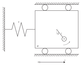
Figure 1: Translational oscillator-rotational actuator scheme

Note that for $u\neq 0$ this system has no equilibria. Consider the following parameters of the system [45]: $J=0.014$, $M=10.5$, $m_{0}=1.5$, $l=0.04$, $k_{\theta}=0.005$, $k=5300$, $k_{1}=5$. For $u=0.48$ the Sommerfeld effect may be observed for initial data $\dot{x}=x=\theta=\dot{\theta}=0$ (zero initial data correspond to typical start of the system, so it was easy to find this effect). But for other initial data $\dot{x}=x=\theta=0,\dot{\theta}=40$ we observe normal operation – the achievement of desired rotational velocity of our mechanical system. In Fig. 2 the transient process for both initial data is shown, in Fig. 2 we observe the attractors which are obtained after the transient process. Note that if we compare this situation to experiment of Sommerfeld we see that an effective level of about 1/4 (comparing to normal operation) is achieved here when Sommerfeld effect takes place.

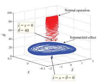
Figure 2: Sommerfeld effect and normal operation in TORA

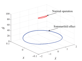
Figure 3: Sommerfeld effect and normal operation in TORA – localization after transient process

3 Drilling systems

Let us consider now another electromechanical system – drilling system. Drilling systems are widely used in oil and gas industry for drilling wells. The failures of drilling systems cause considerable time and expenditure loss for drilling companies, so the understanding of these failures is a very important task. Here we will consider two mathematical models of drilling systems and study their behaviour after operation start. For drilling systems two different ways of operation start are possible: no-load start and start with load. No-load start means that in initial moment of time there is no friction torque acting on the lower disc. Start with load implies start of the drilling with friction torque acting on the lower disc in initial moment of time (this case also corresponds to a sudden change of rock type). In contrast to TORA system these systems have stable equilibrium states which correspond to their normal operation.

3.1 Drilling system actuated by DC motor

The first model of a drilling system was studied in [46, 47]. In these works the scientific group from Eindhoven University of Technology constructed and studied an experimental setup shown in Fig. 4. The configuration of it can be recognised in the structure of drilling systems. The setup consists of two discs connected with a steel string. The upper disc represents rotary table of the drilling system and is actuated by a DC-motor. The lower disc represents bottom hole assembly. It is also assumed that the drill string in massless ad experiences only torsional deformation. The system is described by the following equations:

$$\begin{array}[]{l}J_{u}\ddot{\theta}_{u}+k_{\theta}\left(\theta_{u}-\theta_{l}\right)+b\left(\dot{\theta}_{u}-\dot{\theta}_{l}\right)+T_{fu}\left(\dot{\theta}_{u}\right)-k_{m}v=0,\\ J_{l}\ddot{\theta}_{l}-k_{\theta}\left(\theta_{u}-\theta_{l}\right)-b\left(\dot{\theta}_{u}-\dot{\theta}_{l}\right)+T_{fl}\left(\dot{\theta}_{l}\right)=0.\end{array}$$ (2)

where $\theta_{u}(t)$ and $\theta_{l}(t)$ are angular displacements of the upper and lower discs with respect to the earth, $J_{u}$ and $J_{l}$ are constant inertia torques, $b$ is rotational friction, $k_{\theta}$ is the torsional spring stiffness, $k_{m}$ is the motor constant, $v$ is the constant input voltage. $T_{fu}$ and $T_{fl}$ are friction torques acting on the upper and on the lower disc respectively. Both friction torques $T_{fu}$ and $T_{fl}$ are obtained experimentally.

$$T_{fu}(\dot{\theta}_{u})\in\left\{\begin{array}[]{ll}T_{cu}(\dot{\theta}_{u}){\rm sign}(\dot{\theta}_{u}),&\dot{\theta}_{u}\neq 0\\ \left[-T_{su}+\Delta T_{su},T_{su}+\Delta T_{su}\right],&\dot{\theta}_{u}=0,\end{array}\right.$$ (3)

where

$$T_{cu}(\dot{\theta}_{u})=T_{su}+\Delta T_{su}{\rm sign}(\dot{\theta}_{u})+b_{u}|\dot{\theta}_{u}|+\Delta b_{u}\dot{\theta}_{u}.$$ (4)

and

$$T_{fl}(\dot{\theta}_{l})\in\left\{\begin{array}[]{ll}T_{cl}(\dot{\theta}_{l}){\rm sign}(\dot{\theta}_{l}),&\dot{\theta}_{l}\neq 0\\ \left[-T_{0},T_{0}\right],&\dot{\theta}_{l}=0,\end{array}\right.$$ (5)

where

$$T_{cl}(\dot{\theta}_{l})=\frac{T_{0}}{T_{sl}}(T_{pl}+(T_{sl}-T_{pl})e^{-|\frac{\dot{\theta}_{l}}{\omega_{sl}}|^{\delta_{sl}}}+b_{|}\dot{\theta}_{l}).$$ (6)

Here $T_{su}$, $\Delta T_{su}$, $b_{u}$, $\Delta b_{u}$, $T_{0}$, $T{sl}$, $T_{pl}$, $\omega_{sl}$, $\delta_{sl}$, $b_{l}$ are constant parameters. Note that $T_{fu}$ and $T_{fl}$ are multi-valued functions, so special methods for numerical modelling of (2) are needed (see [48, 49]).

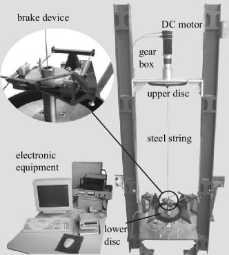
Figure 4: Drilling system setup [46]

Normal operation of the drilling system corresponds to rotation of both upper and lower discs with the same angular velocity with constant angular speed (i.e. the system reaches stable equilibrium state). Instead normal operation system may experience unwanted oscillations which lead to its failures. For modelling (2) we use the following parameters [46]: $k_{m}=4.3228$, $J_{u}=0.4765$, $T_{su}=0.37975$, $\Delta T_{su}=-0.00575$, $b_{u}=2.4245$, $\Delta b_{u}=-0.0084$, $k_{\theta}=0.075$, $b=0$, $J_{l}=0.035$, $T_{sl}=0.26$, $T_{pl}=0.05$, $\omega_{sl}=2.2$, $\delta_{sl}=1.5$, $b_{l}=0.09$. For initial data $\theta_{u}-\theta_{l}=0$, $\dot{\theta}_{u}=\dot{\theta}_{l}=6.1$ (both upper and lower discs rotate with the same angular speed without angular displacement) after transient process the system enters normal operation mode (see Fig. 5). But for same parameters and initial data $\theta_{u}-\theta_{l}=\dot{\theta}_{u}=\dot{\theta}_{l}=0$ (initially discs don’t rotate and there is no angular displacement between them) after transient process the system starts to experience stable hidden oscillations.

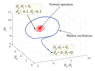
Figure 5: Hidden oscillations and normal operation (corresponds to stable equilibrium state) in drilling system with DC motor

3.2 Drilling system actuated by induction motor

Consider now the modification of the drilling system studied above. Suppose it is driven by an induction motor (see schematic view of the system on Fig. 7). In order to take into account the dynamics of the motor we write the equations in the following form [50, 23, 49]:

$$\begin{array}[]{l}J_{u}\ddot{\theta}_{u}+k_{\theta}\left(\theta_{u}-\theta_{l}\right)+b\left(\dot{\theta}_{u}-\dot{\theta}_{l}\right)\\ -nBS\sum\limits_{k=1}^{3}i_{k}\sin\left(\theta_{u}+\frac{2(k-1)\pi}{3}\right)=0,\cr J_{l}\ddot{\theta_{l}}-k_{\theta}\left(\theta_{u}-\theta_{l}\right)-b\left(\dot{\theta}_{u}-\dot{\theta}_{l}\right)+T_{fl}\left(\omega+\dot{\theta_{l}}\right)=0,\cr L\dot{i}_{1}+(R+r)i_{1}=-nBS\dot{\theta}_{u}\sin\theta_{u},\cr L\dot{i}_{2}+(R+r)i_{2}=-nBS\dot{\theta}_{u}\sin\left(\theta_{u}+\frac{2\pi}{3}\right),\cr L\dot{i}_{3}+(R+r)i_{3}=-nBS\dot{\theta}_{u}\sin\left(\theta_{u}+\frac{4\pi}{3}\right),\end{array}$$ (7)

where $\theta_{u}(t)$ and $\theta_{l}(t)$ are angular displacements of the upper and lower discs with respect to the magnetic field rotating with constant speed $\omega=2\pi f/p$, where $f$ is the motor supply frequency, $p$ is the number of pairs of poles (usually not less than 8 pairs) [51]; $n$ is the number of turns in each coil; $B$ is an induction of magnetic field; $S$ is an area of one turn of coil; $i_{k}$ are currents in coils; $R$ is resistance of each coil; $r$ – variable external resistance; $L$ – inductance of each coil; $J$ – the moment of inertia of the rotor. Note that here angular displacements of the upper and lower discs with respect to the earth are $\theta_{u}(t)+\omega t$ and $\theta_{l}(t)+\omega t$. Friction torque $T_{fl}$ acting on the lower disc is defined in the same way as in the previous model:

$$T_{fl}(\dot{\theta}_{l}+\omega)\in\left\{\begin{array}[]{ll}T_{cl}(\dot{\theta}_{l}+\omega){\rm sign}(\dot{\theta}_{l}+\omega),&\dot{\theta}_{l}+\omega\neq 0\\ \left[-T_{0},T_{0}\right],&\dot{\theta}_{l}+\omega=0,\end{array}\right.$$ (8)

where

$$T_{cl}(\dot{\theta}_{l}+\omega)=\frac{T_{0}}{T_{sl}}(T_{pl}+(T_{sl}-T_{pl})e^{-|\frac{\dot{\theta}_{l}+\omega}{\omega_{sl}}|^{\delta_{sl}}}+b_{l}(\dot{\theta}_{l}+\omega)).$$ (9)

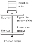
Figure 6: Mathematical model of drilling system actuated by induction motor

Let us model the system (7) with the following parameters: $T_{0}=0.25$, $c=10$, $\omega=8$, $J_{u}=0.4765$, $J_{l}=0.035$, $k=0.075$, $a=2.1$, $b=0$, $T_{sl}=0.26$, $T_{pl}=0.05$, $\omega_{sl}=2.2$, $\delta_{sl}=1.5$, $b_{l}=0.009$. For initial data $\theta$=$\theta_{u}-\theta_{l}$=0, $\omega_{u}=-\dot{\theta}_{u}=0$ and $\omega_{l}=-\dot{\theta}_{l}=0$ (rotation of both discs with the same speed without angular displacement) after the transient process the drilling system enters normal operation mode (see Fig. 7). But for initial data $\theta$=0, $\omega_{u}=8$ and $\omega_{l}=8$ (initially discs don’t rotate and there is no angular displacement) after the transient process the system starts to experience hidden oscillations, which may lead to break-down.

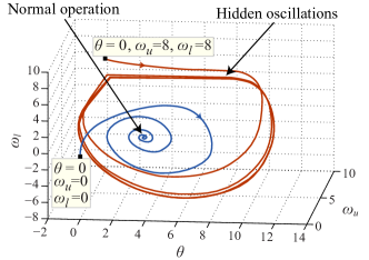
Figure 7: Hidden oscillations and normal operation (corresponds to stable equilibrium state) in drilling system actuated by induction motor

4 Conclusions

We modelled three different electromechanical systems. All of them have hidden oscillations in sense of mathematical definition. But from physical point of view some of these oscillations are easily localized, thus are not actually hidden. For example, for TORA system zero initial data correspond to typical start of the system, so Sommerfeld effect can be easily localized. In our examples for drilling systems no-load start leads to normal operation and start with load (or change of rock type) leads to unwanted hidden oscillations. Hence better understanding of physical nature of operation of electromechanical models may make it easier to find hidden attractors.

References

- [1] N. V. Kuznetsov, G. A. Leonov, V. I. Vagaitsev, Analytical-numerical method for attractor localization of generalized Chua’s system, IFAC Proceedings Volumes (IFAC-PapersOnline) 4 (1) (2010) 29–33. doi:10.3182/20100826-3-TR-4016.00009.
- [2] G. A. Leonov, N. V. Kuznetsov, V. I. Vagaitsev, Localization of hidden Chua’s attractors, Physics Letters A 375 (23) (2011) 2230–2233. doi:10.1016/j.physleta.2011.04.037.
- [3] G. A. Leonov, N. V. Kuznetsov, V. I. Vagaitsev, Hidden attractor in smooth Chua systems, Physica D: Nonlinear Phenomena 241 (18) (2012) 1482–1486. doi:10.1016/j.physd.2012.05.016.
- [4] G. A. Leonov, N. V. Kuznetsov, Hidden attractors in dynamical systems. From hidden oscillations in Hilbert-Kolmogorov, Aizerman, and Kalman problems to hidden chaotic attractors in Chua circuits, International Journal of Bifurcation and Chaos 23 (1), art. no. 1330002. doi:10.1142/S0218127413300024.
- [5] G. Leonov, N. Kuznetsov, T. Mokaev, Homoclinic orbits, and self-excited and hidden attractors in a Lorenz-like system describing convective fluid motion, Eur. Phys. J. Special Topics 224 (8) (2015) 1421–1458. doi:10.1140/epjst/e2015-02470-3.
- [6] M. Shahzad, V.-T. Pham, M. Ahmad, S. Jafari, F. Hadaeghi, Synchronization and circuit design of a chaotic system with coexisting hidden attractors, European Physical Journal: Special Topics 224 (8) (2015) 1637–1652.
- [7] S. Brezetskyi, D. Dudkowski, T. Kapitaniak, Rare and hidden attractors in van der Pol-Duffing oscillators, European Physical Journal: Special Topics 224 (8) (2015) 1459–1467.
- [8] S. Jafari, J. Sprott, F. Nazarimehr, Recent new examples of hidden attractors, European Physical Journal: Special Topics 224 (8) (2015) 1469–1476.
- [9] Z. Zhusubaliyev, E. Mosekilde, A. Churilov, A. Medvedev, Multistability and hidden attractors in an impulsive Goodwin oscillator with time delay, European Physical Journal: Special Topics 224 (8) (2015) 1519–1539.
- [10] P. Saha, D. Saha, A. Ray, A. Chowdhury, Memristive non-linear system and hidden attractor, European Physical Journal: Special Topics 224 (8) (2015) 1563–1574.
- [11] V. Semenov, I. Korneev, P. Arinushkin, G. Strelkova, T. Vadivasova, V. Anishchenko, Numerical and experimental studies of attractors in memristor-based Chua’s oscillator with a line of equilibria. Noise-induced effects, European Physical Journal: Special Topics 224 (8) (2015) 1553–1561.
- [12] Y. Feng, Z. Wei, Delayed feedback control and bifurcation analysis of the generalized Sprott B system with hidden attractors, European Physical Journal: Special Topics 224 (8) (2015) 1619–1636.
- [13] C. Li, W. Hu, J. Sprott, X. Wang, Multistability in symmetric chaotic systems, European Physical Journal: Special Topics 224 (8) (2015) 1493–1506.
- [14] Y. Feng, J. Pu, Z. Wei, Switched generalized function projective synchronization of two hyperchaotic systems with hidden attractors, European Physical Journal: Special Topics 224 (8) (2015) 1593–1604.
- [15] J. Sprott, Strange attractors with various equilibrium types, European Physical Journal: Special Topics 224 (8) (2015) 1409–1419.
- [16] V. Pham, S. Vaidyanathan, C. Volos, S. Jafari, Hidden attractors in a chaotic system with an exponential nonlinear term, European Physical Journal: Special Topics 224 (8) (2015) 1507–1517.
- [17] S. Vaidyanathan, V.-T. Pham, C. Volos, A 5-D hyperchaotic Rikitake dynamo system with hidden attractors, European Physical Journal: Special Topics 224 (8) (2015) 1575–1592.
- [18] P. Sharma, M. Shrimali, A. Prasad, N. Kuznetsov, G. Leonov, Control of multistability in hidden attractors, Eur. Phys. J. Special Topics 224 (8) (2015) 1485–1491.
- [19] N. V. Kuznetsov, O. A. Kuznetsova, G. A. Leonov, Visualization of four normal size limit cycles in two-dimensional polynomial quadratic system, Differential equations and dynamical systems 21 (1-2) (2013) 29–34. doi:10.1007/s12591-012-0118-6.
- [20] G. A. Leonov, N. V. Kuznetsov, Algorithms for searching for hidden oscillations in the Aizerman and Kalman problems, Doklady Mathematics 84 (1) (2011) 475–481. doi:10.1134/S1064562411040120.
- [21] V. O. Bragin, V. I. Vagaitsev, N. V. Kuznetsov, G. A. Leonov, Algorithms for finding hidden oscillations in nonlinear systems. The Aizerman and Kalman conjectures and Chua’s circuits, Journal of Computer and Systems Sciences International 50 (4) (2011) 511–543. doi:10.1134/S106423071104006X.
- [22] B. R. Andrievsky, N. V. Kuznetsov, G. A. Leonov, A. Y. Pogromsky, Hidden oscillations in aircraft flight control system with input saturation, IFAC Proceedings Volumes (IFAC-PapersOnline) 5 (1) (2013) 75–79. doi:10.3182/20130703-3-FR-4039.00026.
- [23] G. A. Leonov, N. V. Kuznetsov, M. A. Kiseleva, E. P. Solovyeva, A. M. Zaretskiy, Hidden oscillations in mathematical model of drilling system actuated by induction motor with a wound rotor, Nonlinear Dynamics 77 (1-2) (2014) 277–288. doi:10.1007/s11071-014-1292-6.
- [24] N. Kuznetsov, G. Leonov, Hidden attractors in dynamical systems: systems with no equilibria, multistability and coexisting attractors, IFAC Proceedings Volumes (IFAC-PapersOnline) 19 (2014) 5445–5454. doi:10.3182/20140824-6-ZA-1003.02501.
- [25] G. Bianchi, N. Kuznetsov, G. Leonov, M. Yuldashev, R. Yuldashev, Limitations of PLL simulation: hidden oscillations in MATLAB and SPICE, in: 2015 7th International Congress on Ultra Modern Telecommunications and Control Systems and Workshops (ICUMT), 2015, pp. 79–84, http://arxiv.org/pdf/1506.02484.pdf, http://www.mathworks.com/matlabcentral/fileexchange/52419-hidden-oscillations-in-pll.
- [26] G. Leonov, M. Kiseleva, N. Kuznetsov, O. Kuznetsova, Discontinuous differential equations: comparison of solution definitions and localization of hidden Chua attractors, IFAC-PapersOnLine 48 (11) (2015) 408–413. doi:10.1016/j.ifacol.2015.09.220.
- [27] N. Kuznetsov, Hidden attractors in fundamental problems and engineering models. A short survey., AETA 2015: Recent Advances in Electrical Engineering and Related Sciences, Lecture Notes in Electrical Engineering 371 (2016) 13–25. doi:0.1007/978-3-319-27247-4\_2.
- [28] S. Kingni, S. Jafari, H. Simo, P. Woafo, Three-dimensional chaotic autonomous system with only one stable equilibrium: Analysis, circuit design, parameter estimation, control, synchronization and its fractional-order form, The European Physical Journal Plus 129 (5).
- [29] I. Burkin, N. Khien, Analytical-numerical methods of finding hidden oscillations in multidimensional dynamical systems, Differential Equations 50 (13) (2014) 1695–1717.
- [30] V.-T. Pham, F. Rahma, M. Frasca, L. Fortuna, Dynamics and synchronization of a novel hyperchaotic system without equilibrium, International Journal of Bifurcation and Chaos 24 (06), art. num. 1450087.
- [31] D. Cafagna, G. Grassi, Fractional-order systems without equilibria: The first example of hyperchaos and its application to synchronization, Chinese Physics B 24 (8) (2015) 080502.
- [32] Z. Wang, W. Sun, Z. Wei, S. Zhang, Dynamics and delayed feedback control for a 3d jerk system with hidden attractor, Nonlinear Dynamicsdoi:10.1007/s11071-015-2177-z.
- [33] A. Kuznetsov, S. Kuznetsov, E. Mosekilde, N. Stankevich, Co-existing hidden attractors in a radio-physical oscillator system, Journal of Physics A: Mathematical and Theoretical 48 (2015) 125101.
- [34] I. Zelinka, Evolutionary identification of hidden chaotic attractors, Engineering Applications of Artificial Intelligence10.1016/j.engappai.2015.12.002.
- [35] G. Chen, Chaotic systems with any number of equilibria and their hidden attractors (plenary lecture), in: 4th IFAC Conference on Analysis and Control of Chaotic Systems, 2015, http://www.ee.cityu.edu.hk/gchen/pdf/CHEN_IFAC2015.pdf.
- [36] B. Bao, F. Hu, M. Chen, Q. Xu, Y. Yu, Self-excited and hidden attractors found simultaneously in a modified Chua’s circuit, International Journal of Bifurcation and Chaos 25 (05) (2015) 1550075. doi:10.1142/S0218127415500753.
- [37] A. Sommerfeld, Beitrage zum dynamischen ausbau der festigkeitslehre, Zeitschrift des Vereins deutscher Ingenieure 46 (1902) 391–394.
- [38] R. Evan-Iwanowski, Resonance Oscillations in Mechanical Systems, Elsevier, 1976.
- [39] M. Eckert, Arnold Sommerfeld: Science, Life and Turbulent Times 1868-1951, Springer, 2013.
- [40] S. Nose, A molecular dynamics method for simulations in the canonical ensemble, Molecular Physics 52 (2) (1984) 255–268.
- [41] W. Hoover, Canonical dynamics: Equilibrium phase-space distributions, Phys. Rev. A 31 (1985) 1695–1697.
- [42] J. Sprott, Some simple chaotic flows, Physical Review E 50 (2) (1994) R647–R650.
- [43] X.-S. Y. Lei Wang, The invariant tori of knot type and the interlinked invariant tori in the nose-hoover oscillator, The European Physical Journal B 88, art. num. 78.
- [44] V. Venkatasubramanian, Stable operation of a simple power system with no equilibrium points, in: Proceedings of the 40th IEEE Conference on Decision and Control, Vol. 3, 2001, pp. 2201–2203.
- [45] A. Fradkov, O. Tomchina, D. Tomchin, Controlled passage through resonance in mechanical systems, Journal of Sound and Vibration 330 (6) (2011) 1065–1073.
- [46] J. de Bruin, A. Doris, N. van de Wouw, W. Heemels, H. Nijmeijer, Control of mechanical motion systems with non-collocation of actuation and friction: A Popov criterion approach for input-to-state stability and set-valued nonlinearities, Automatica 45 (2) (2009) 405–415.
- [47] N. Mihajlovic, A. van Veggel, N. van de Wouw, H. Nijmeijer, Analysis of friction-induced limit cycling in an experimental drill-string system, J. Dyn. Syst. Meas. Control 126 (4) (2004) 709–720.
- [48] P. T. Piiroinen, Y. A. Kuznetsov, An event-driven method to simulate filippov systems with accurate computing of sliding motions, ACM Transactions on Mathematical Software (TOMS) 34 (3) (2008) 13.
- [49] M. Kiseleva, Oscillations of Dynamical Systems Applied in Drilling Analytical and Numerical Methods, Jyväskylä University Printing House, 2013.
- [50] M. Kiseleva, N. Kondratyeva, N. Kuznetsov, G. Leonov, E. Solovyeva, Hidden periodic oscillations in drilling system driven by induction motor, IFAC Proceedings Volumes (IFAC-PapersOnline) 19 (2014) 5872–5877.
- [51] W. Leonhard, Control of electrical drives, Springer, 2001.