Stability of the superconducting $d_{x^{2}-y^{2}}$-wave pairing towards the intersite Coulomb repulsion… Stability of the superconducting $d_{x^{2}-y^{2}}$-wave pairing towards the intersite Coulomb repulsion between oxygen holes in high-T_c superconductors V. V. Val’kov, D. M. Dzebisashvili, M. M. Korovushkin, and A. F. Barabanov

Stability of the superconducting $d_{x^{2}-y^{2}}$-wave pairing towards the intersite Coulomb repulsion between oxygen holes in high-T_c superconductors

Abstract

It is shown that an account for the space separatedness of the two-orbital subsystem of the oxygen holes and the subsystem of the localized spins of copper ions in high-T_c cuprate superconductors leads to the stability of the superconducting $d_{x^{2}-y^{2}}$-wave pairing towards the strong Coulomb repulsion between holes located at the nearest oxygen ions. This effect is due to the fact that the Coulomb potential slips out of the equation for the Cooper pairing in the $d_{x^{2}-y^{2}}$-wave channel owing to the properties of symmetry.

71.10.Fd, 71.27.+a, 74.20.Mn, 74.20.-z, 74.72.Gh

1. Introduction

It is known that the Cooper pairing of the fermions resulting from the kinematic [1], exchange and spin-fluctuation [2, 3] mechanisms, which are considered in the framework of the Hubbard model [4, 5, 6], $t-J$ model [2, 3, 7], and $t-J^{*}$ model [8, 9, 10], is suppressed with regard to the intersite Coulomb interaction $V$ between the carriers located at the nearest sites of the lattice. This effect manifests itself most strongly in the $d$-wave channel [12], so at the values $V\sim 1-2~{}\mathrm{eV}$ [11] the Cooper instability is turned out to be totally suppressed. The $s$-wave pairing caused by the stronger kinematic mechanism [1] is more stable and, as a result, the Cooper pairing is robust even with regard to $V$ [4, 5, 6]. Thus, the contradiction between the theoretical and experimental results arises: an account for the Coulomb repulsion leads to the suppression of the $d$-wave pairing, which is experimentally observed, but maintains the $s$-wave pairing, which is not realized in the experiment. This fact significantly restricts the capabilities of the above-mentioned theories of high-T_c superconductors.

In this paper, it is shown that an account for the real structure of CuO₂ plane in the framework of the Emery model [13, 14] removes the above-mentioned contradiction. In our theory, the Fourier transform corresponding to the Coulomb repulsion between the holes located at the nearest oxygen sites slips out of the equation for the Cooper pairing in the $d$-wave channel owing to the properties of symmetry. At the same time, the self-consistent equation for the $s$-wave pairing contains the contribution of the Coulomb interaction and, as a result, this pairing is suppressed. Thus, our theory answers the question of why the superconducting $d$-wave pairing survives with regard to the intersite Coulomb repulsion between oxygen holes, as well as why the $d_{x^{2}-y^{2}}$-wave pairing instead of the $s$-wave pairing occurs in cuprate superconductors.

2. The spin-fermion model

In the regime of the strong electron correlations, in which the Hubbard repulsion between holes $U_{d}$ is large, i.e., $U_{d}>\Delta_{pd}\gg t_{pd}$, the Emery model can be reduced to the spin-fermion model [15, 16] with the Hamiltonian

$$\hat{H}=\hat{H}_{0}+\hat{J}+\hat{V}+\hat{I},$$ (1)

$$\hat{H}_{0}=\sum_{k\alpha}\Bigl{(}\xi_{0}(k_{x})a_{k\alpha}^{\dagger}a_{k\alpha}+\xi_{0}(k_{y})b_{k\alpha}^{\dagger}b_{k\alpha}+$$

$$\qquad+t_{k}(a_{k\alpha}^{\dagger}b_{k\alpha}+b_{k\alpha}^{\dagger}a_{k\alpha})\Bigr{)},$$

$$\hat{J}=\frac{J}{N}\sum_{\begin{subarray}{c}fkq\\ \alpha\beta\end{subarray}}e^{if(q-k)}u_{k\alpha}^{{\dagger}}(\textbf{S}_{f}\boldsymbol{\sigma}_{\alpha\beta})u_{q\beta},$$

$$\hat{V}=V\sum_{f\Delta}\hat{n}_{f+\frac{x}{2}}\hat{n}_{f+\frac{x}{2}+\Delta},\qquad\hat{I}=\frac{I}{2}\sum_{\langle fm\rangle}\textbf{S}_{f}\textbf{S}_{m},$$

which describes the subsystem of the oxygen holes interacting with the localized spins in copper ions. Here

$$\xi_{0}(k_{x(y)})=\varepsilon_{p}-\mu+\tau(1+\cos k_{x(y)}),$$

$$t_{k}=(2\tau-4t)\cos\frac{k_{x}}{2}\cos\frac{k_{y}}{2},$$

$$u_{k\beta}=\cos\frac{k_{x}}{2}a_{k\beta}+\cos\frac{k_{y}}{2}b_{k\beta},$$

$$\tau=\frac{t_{pd}^{2}}{\Delta_{pd}}\biggl{(}1-\frac{\Delta_{pd}}{U_{d}-\Delta_{pd}-2V_{pd}}\biggr{)},$$

$$J=\frac{4t_{pd}^{2}}{\Delta_{pd}}\biggl{(}1+\frac{\Delta_{pd}}{U_{d}-\Delta_{pd}-2V_{pd}}\biggr{)},$$

$$I=\frac{4t_{pd}^{4}}{(\Delta_{pd}+V_{pd})^{2}}\biggl{(}\frac{1}{U_{d}}+\frac{2}{2\Delta_{pd}+U_{p}}\biggr{)}.$$ (2)

The Hamiltonian $\hat{H}_{0}$ describes the subsystem of oxygen holes in the momentum representation. The operators $a_{k\alpha}^{\dagger}(a_{k\alpha})$ create (annihilate) the holes with spin $\alpha=\pm 1/2$ in the oxygen subsystem with the $p_{x}$-orbitals. Similarly, the operators $b_{k\alpha}^{\dagger}(b_{k\alpha})$ operate in the oxygen subsystem with the $p_{y}$-orbitals. The initial one-site energy of holes is $\varepsilon_{p}$; $\mu$ is the chemical potential; $t$ is hopping parameter of the oxygen holes. The exchange interaction between the oxygen subsystem and the subsystem of the localized spins is described by the operator $\hat{J}$. Here, $\textbf{S}_{f}$ is the vector operator of the spin moment on the copper ion in the site with index $f$ and $\boldsymbol{\sigma}=(\sigma^{x},\,\sigma^{y},\,\sigma^{z})$ is the vector that consists of the Pauli matrices. The Coulomb interaction between holes located at the nearest oxygen ions is described by the operator $\hat{V}$. Here, $\hat{n}_{f+x(y)/2}=\sum_{\sigma}\hat{n}_{f+x(y)/2,\sigma}$ is the operator of the number of holes at the oxygen ion with index $f+x(y)/2$ ; $\textbf{x}=(1,0)$ and $\textbf{y}=(0,1)$ are lattice basis vectors in the units of the lattice parameter; $\Delta$ is a vector connecting the nearest oxygen ions. The last term of the Hamiltonian describes the exchange interaction between the nearest spins of copper ions. The intensity of this interaction is giving by the parameter $I$.

Below we use the following commonly accepted parameter values: $t_{pd}=1.3\,\textrm{eV}$, $\Delta_{pd}=3.6\,\textrm{eV}$, $U_{d}=10.5\,\textrm{eV}$, $V_{pd}=1.2\,\textrm{eV}$, $V=1-2\,\textrm{eV}$ [17, 18, 11]. For these values the parameter of exchange interaction $I~{}=~{}0.136\,\textrm{eV}\,(1570\,\textrm{K})$ agrees well with the available experimental data [18]. For the hopping parameter of the oxygen holes, we use the value $t=0.1\,\textrm{eV}$.

Note that the value of the exchange interaction between the oxygen subsystem and the subsystem of the localized spins calculated using the expression (Stability of the superconducting $d_{x^{2}-y^{2}}$-wave pairing towards the intersite Coulomb repulsion between oxygen holes in high-T_c superconductors) is turned out to be large: $J=3.4\,\textrm{eV}\gg\tau\approx 0.1\,\textrm{eV}$. Thus, the dynamics of the oxygen holes should be described taking into account their correlation with the subsystem of spins of copper ions. This problem can be solved using the basis set of operators [19, 20]

$$a_{k\alpha},\quad b_{k\alpha},\quad L_{k\alpha}=\frac{1}{N}\sum_{fq\beta}e^{if(q-k)}(\textbf{S}_{f}\boldsymbol{\sigma}_{\alpha\beta})u_{q\beta},$$ (3)

where the third operator couples both the spin and the fermion dynamics.

3. Equations for Green’s functions

To consider the conditions for the Cooper instability, let us add the operators ($\bar{\alpha}=-\alpha$)

$$a_{-k\bar{\alpha}}^{{\dagger}},\quad b_{-k\bar{\alpha}}^{{\dagger}},\quad L_{-k\bar{\alpha}}^{{\dagger}}$$ (4)

to the basis set (3). The system of equations for the normal $G_{ij}$ and the anomalous $F_{ij}$ Green’s functions obtained in the framework of the method [21, 22] can be written as follows ($j=1,2,3$)

$$(\omega-\xi_{x})G_{1j}=\delta_{1j}+t_{k}G_{2j}+J_{x}G_{3j}+\Delta_{1k}F_{2j},$$

$$(\omega-\xi_{y})G_{2j}=\delta_{2j}+t_{k}G_{1j}+J_{y}G_{3j}+\Delta_{2k}F_{1j},$$

$$(\omega-\xi_{3})G_{3j}=\delta_{3j}K_{k}+(J_{x}G_{1j}+J_{y}G_{2j})K_{k}+\Delta_{3k}F_{3j},$$

$$(\omega+\xi_{x})F_{1j}=\Delta_{2k}^{*}G_{2j}-t_{k}F_{2j}-J_{x}F_{3j},$$

$$(\omega+\xi_{y})F_{2j}=\Delta_{1k}^{*}G_{1j}-t_{k}F_{1j}-J_{y}F_{3j},$$

$$(\omega+\xi_{3})F_{3j}=\Delta^{*}_{3k}G_{3j}-(J_{x}F_{1j}+J_{y}F_{2j})K_{k}.$$ (5)

Here the defenitions

$$G_{11}=\langle\langle a_{k\uparrow}|a_{k\uparrow}^{{\dagger}}\rangle\rangle,~{}G_{21}=\langle\langle b_{k\uparrow}|a_{k\uparrow}^{{\dagger}}\rangle\rangle,~{}G_{31}=\langle\langle L_{k\uparrow}|a_{k\uparrow}^{{\dagger}}\rangle\rangle.$$

are used. The functions $G_{i2}$ and $G_{i3}$ are defined similarly, with the difference that instead $a^{{\dagger}}_{k\uparrow}$ the operators $b^{{\dagger}}_{k\uparrow}$ and $L^{{\dagger}}_{k\uparrow}$ stand, respectively. The anomalous Green’s functions are

$$F_{11}=\langle\langle a_{-k\downarrow}^{{\dagger}}|a_{k\uparrow}^{{\dagger}}\rangle\rangle,\,F_{21}=\langle\langle b_{-k\downarrow}^{{\dagger}}|a_{k\uparrow}^{{\dagger}}\rangle\rangle,\,F_{31}=\langle\langle L_{-k\downarrow}^{{\dagger}}|a_{k\uparrow}^{{\dagger}}\rangle\rangle.$$

At that, for $F_{i2}$ and $F_{i3}$ the same definitions regarding the second index are used. The functions in (Stability of the superconducting $d_{x^{2}-y^{2}}$-wave pairing towards the intersite Coulomb repulsion between oxygen holes in high-T_c superconductors) are

$$\xi_{x(y)}=\xi_{0}({k_{x(y)}})+4n_{p}V,$$

$$J_{x(y)}=J\cos\frac{k_{x(y)}}{2},\quad K_{k}=3/4+C_{1}\gamma_{1k},$$

$$\xi_{3}=\varepsilon_{p}-\mu-2t+5\tau/2-J+n_{p}V+$$

$$\quad+\left[(\tau-2t)(C_{1}\gamma_{1k}+C_{2}\gamma_{2k})+\tau(C_{1}\gamma_{1k}+C_{3}\gamma_{3k})/2\right.+$$

$$\quad\left.+JC_{1}(1-4\gamma_{1k})/4+IC_{1}(\gamma_{1k}-4)\right]K_{k}^{-1}.$$ (6)

Here, the number of holes per one oxygen ion is $n_{p}$, $\gamma_{jk}$ are the square lattice invariants: $\gamma_{1k}=(\cos k_{x}+\cos k_{y})/2,\quad\gamma_{2k}=\cos k_{x}\,\cos k_{y},\quad\gamma_{3k}=(\cos 2k_{x}+\cos 2k_{y})/2$. To obtain (Stability of the superconducting $d_{x^{2}-y^{2}}$-wave pairing towards the intersite Coulomb repulsion between oxygen holes in high-T_c superconductors), we assume that the subsystem of the localized spins is in the quantum spin liquid state. In this case, the spin correlation functions $C_{j}=\langle\textbf{S}_{0}\textbf{S}_{r_{j}}\rangle$ satisfy the relations

$$C_{j}=3\langle S^{x}_{0}S^{x}_{r_{j}}\rangle=3\langle S^{y}_{0}S^{y}_{r_{j}}\rangle=3\langle S^{z}_{0}S^{z}_{r_{j}}\rangle,$$ (7)

where $r_{j}$ is a coordinate of the copper ion in the coordination sphere $j$. At that, $\langle S^{x}_{f}\rangle=\langle S^{y}_{f}\rangle=\langle S^{z}_{f}\rangle=0$.

Using system (Stability of the superconducting $d_{x^{2}-y^{2}}$-wave pairing towards the intersite Coulomb repulsion between oxygen holes in high-T_c superconductors), one can obtain that the fermionic spectrum in the normal phase can be obtained from the dispersion equation

$$\mathrm{det}_{k}(\omega)=(\omega-\xi_{x})(\omega-\xi_{y})(\omega-\xi_{3})-2J_{x}J_{y}t_{k}K_{k}-$$

$$-(\omega-\xi_{y})J_{x}^{2}K_{k}-(\omega-\xi_{x})J_{y}^{2}K_{k}-(\omega-\xi_{3})t_{k}^{2}=0.$$ (8)

The spectrum consists of the three branches $\epsilon_{1k}$, $\epsilon_{2k}$ and $\epsilon_{3k}$ [23]. The appearing of the branch $\epsilon_{1k}$ with the minimum near ($\pi/2$, $\pi/2$) is caused by the strong spin-fermionic correlation which initiates both the exchange interaction between the hole and the nearest copper ions and the spin-correlated hoppings. At the low number $n_{p}$, the dynamics of holes is mainly defined by the lower band $\epsilon_{1k}$, which is significantly separated from the upper bands $\epsilon_{2k}$ and $\epsilon_{3k}$ [23].

The superconducting order parameters $\Delta_{j,k}$ are connected with the anomalous averages by means the following expressions ($C_{1x(1y)}=C_{1}\cos^{2}(q_{x(y)}/2)$):

$$\Delta_{1k}=-\frac{4V}{N}\sum_{q}\phi_{k-q}\langle a_{q\uparrow}b_{-q\downarrow}\rangle,~{}~{}~{}\phi_{k}=\displaystyle\cos\frac{k_{x}}{2}\cos\frac{k_{y}}{2},$$

$$\Delta_{2k}=-\frac{4V}{N}\sum_{q}\phi_{k-q}\langle b_{q\uparrow}a_{-q\downarrow}\rangle,$$ (9)

$$\Delta_{3k}=\frac{1}{N}\sum_{q}\biggl{\{}I_{k-q}\Bigl{[}\langle L_{q\uparrow}L_{-q\downarrow}\rangle-$$

$$\quad-C_{1x}\langle a_{q\uparrow}a_{-q\downarrow}\rangle-C_{1y}\langle b_{q\uparrow}b_{-q\downarrow}\rangle\Bigr{]}K_{k}^{-1}+$$

$$\quad+(\widetilde{V}_{k}-C_{1}I_{k-q}K_{k}^{-1})\phi_{q}\bigl{(}\langle a_{q\uparrow}b_{-q\downarrow}\rangle+\langle b_{q\uparrow}a_{-q\downarrow}\rangle\bigr{)}\biggr{\}}.$$

Here $\widetilde{V}_{k}=V\left(1+(C_{1}\gamma_{1k}+C_{2}\gamma_{2k})K_{k}^{-1}\right)$.

4. The system of equations for the superconducting order parameters

To analyze the conditions for the Cooper instability, let us express in the linear approximation the anomalous Green’s functions in terms of the parameters $\Delta^{*}_{jk}$

$$F_{nm}(k,\omega)=\sum_{j=1}^{3}S^{(j)}_{nm}(k,\omega)\Delta_{jk}^{*}/\textrm{Det}_{k}(\omega),$$ (10)

where the following notations are used:

$$\textrm{Det}_{k}(\omega)=-\textrm{det}_{k}(\omega)\textrm{det}_{k}(-\omega),$$

$$S^{(1)}_{12}(k,\omega)~{}=~{}S^{(2)}_{21}(k,\omega)~{}=~{}Q_{3}(k,-\omega)Q_{3}(k,\omega),$$

$$S^{(2)}_{12}(k,\omega)=Q_{3y}(k,-\omega)Q_{3x}(k,\omega),$$

$$S^{(3)}_{12}(k,\omega)=K_{k}Q_{y}(k,-\omega)Q_{x}(k,\omega),$$

$$S^{(1)}_{21}(k,\omega)~{}=~{}S^{(2)}_{12}(k,-\omega),~{}~{}S^{(3)}_{21}(k,\omega)~{}=~{}S^{(3)}_{12}(k,-\omega),$$

$$S^{(1)}_{11}(k,\omega)~{}=~{}Q_{3}(k,-\omega)Q_{3y}(k,\omega),$$

$$S^{(2)}_{33}(k,\omega)=K_{k}S^{(3)}_{12}(k,\omega),~{}S^{(2)}_{11}(k,\omega)~{}=~{}S^{(1)}_{11}(k,-\omega),$$

$$S^{(3)}_{11}(k,\omega)=K_{k}Q_{y}(k,-\omega)Q_{y}(k,\omega),$$

$$S^{(1)}_{22}(k,\omega)=Q_{3x}(k,-\omega)Q_{3}(k,\omega),$$

$$S^{(1)}_{33}(k,\omega)=K_{k}S^{(3)}_{21}(k,\omega),~{}S^{(2)}_{22}(k,\omega)=S^{(1)}_{22}(k,-\omega),$$

$$S^{(3)}_{22}(k,\omega)=K_{k}Q_{x}(k,-\omega)Q_{x}(k,\omega),$$

$$S^{(3)}_{33}(k,\omega)=K_{k}Q_{xy}(k,-\omega)Q_{xy}(k,\omega).$$

These expressions include the functions

$$Q_{x(y)}(k,\omega)=(\omega-\xi_{x(y)})J_{y(x)}+t_{k}J_{x(y)},$$

$$Q_{3}(k,\omega)=(\omega-\xi_{3})t_{k}+J_{x}J_{y}K_{k},$$

$$Q_{3x(3y)}(k,\omega)=(\omega-\xi_{3})(\omega-\xi_{x(y)})-J_{x(y)}^{2}K_{k},$$

$$Q_{xy}(k,\omega)=(\omega-\xi_{x})(\omega-\xi_{y})-t_{k}^{2}.$$ (11)

Using the spectral theorem [24], we obtain the expressions for the anomalous averages and the closed system of homogenous integral equations for the superconducting order parameters

$$\Delta_{1k}^{*}=\frac{4V}{N}\sum_{jq}\phi_{k-q}M^{(j)}_{21}(q)\Delta_{jq}^{*},$$

$$\Delta_{2k}^{*}=\frac{4V}{N}\sum_{jq}\phi_{k-q}M^{(j)}_{12}(q)\Delta_{jq}^{*},$$

$$\Delta_{3k}^{*}=\frac{1}{N}\sum_{jq}\left\{\frac{I_{k-q}}{K_{k}}\left[C_{1x}M^{(j)}_{11}(q)+C_{1y}M^{(j)}_{22}(q)-M^{(j)}_{33}(q)\right]\right.$$

$$\qquad\left.+(I_{k-q}C_{1}K_{k}^{-1}-\widetilde{V}_{k})\phi_{q}\left[M^{(j)}_{12}(q)+M^{(j)}_{21}(q)\right]\right\}\Delta_{jq}^{*},$$ (12)

where

$$M^{(j)}_{nm}(q)=\frac{S^{(j)}_{nm}(q,E_{1q})+S^{(j)}_{nm}(q,-E_{1q})}{4E_{1q}(E_{1q}^{2}-E_{2q}^{2})(E_{1q}^{2}-E_{3q}^{2})}\tanh\left(\frac{E_{1q}}{2T}\right).$$

Below, we use the system (Stability of the superconducting $d_{x^{2}-y^{2}}$-wave pairing towards the intersite Coulomb repulsion between oxygen holes in high-T_c superconductors) to find the critical temperature of the transition to the superconducting phase with the assigned type of symmetry of the order parameter.

5. The critical temperature of the superconducting $d_{x^{2}-y^{2}}$-wave pairing

For the superconducting $d_{x^{2}-y^{2}}$-wave pairing, when

$$\Delta_{3k}=\Delta_{0}\cdot(\cos k_{x}-\cos k_{y}),$$ (13)

it follows from the system (Stability of the superconducting $d_{x^{2}-y^{2}}$-wave pairing towards the intersite Coulomb repulsion between oxygen holes in high-T_c superconductors) that $\Delta_{1k}=0$ and $\Delta_{2k}=0$. It is easily seen if one takes into account that the kernels of the integral equations for $\Delta^{*}_{1k}$ and $\Delta^{*}_{2k}$ contain the function $\phi_{k-q}$. As a result, the integration over $q$ vanishes these superconducting order parameters.

It follows from the integral equation for the third superconducting order parameter $\Delta^{*}_{3k}$ that the contribution of the intersite Coulomb potential to the kernel of the integral equation is equal to zero. This is due to the symmetry properties of the integrands and manifests itself after summation over the internal variable. As a result, we find that the Coulomb repulsion between the holes located at the nearest oxygen ions does not suppress the superconducting $d_{x^{2}-y^{2}}$-wave pairing. Thus, we arrive at the equation for the concentration dependence of the critical temperature

$$1=\frac{I}{N}\sum_{q}\frac{(\cos q_{x}-\cos q_{y})^{2}}{2E_{1q}}\Psi_{q}\tanh\biggl{(}\frac{E_{1q}}{2T_{c}}\biggr{)},$$ (14)

where

$$\Psi_{q}=\biggl{\{}S_{33}^{(3)}(E_{1q})-C_{1x}S_{11}^{(3)}(E_{1q})-C_{1y}S_{22}^{(3)}(E_{1q})-$$

$$\quad-C_{1}\phi_{q}\left(S_{12}^{(3)}(E_{1q})+S_{21}^{(3)}(E_{1q})\right)\Bigr{]}\biggr{\}}\times$$ (15)

$$\quad\times\left[K_{q}(E_{1q}^{2}-E_{2q}^{2})(E_{1q}^{2}-E_{3q}^{2})\right]^{-1}.$$

Figure 1 shows the dependencies of the superconducting critical temperature on doping obtained by solving Eq. (14). A comparison of the curves shows that an account for the intersite Coulomb repulsion leads to insignificant and nonuniform in doping modification of the dependence $T_{c}(n)$. Note that these insignificant modifications are caused by the renormalization of the one-site energy of holes owing to the intersite Coulomb repulsion, but not the renormalization of the coupling constant.

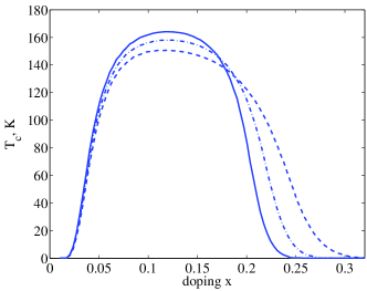
Figure 1: Fig. 1. Concentration dependence of the critical temperature of the transition to the superconducting $d_{x^{2}-y^{2}}$-wave phase calculated for $V=0$ (dotted curve), $V=1\,\textrm{eV}$ (dashed-dotted curve) and $V=2\,\textrm{eV}$ (solid curve).

4. Conclusion

The main result of the paper is connected with the answer to the question of why the superconducting $d$-wave pairing survives with regard to the intersite Coulomb repulsion between oxygen holes, as well as why the $d_{x^{2}-y^{2}}$-wave pairing instead of the $s$-wave pairing occurs in cuprate superconductors despite the strong coupling constant which corresponds to the kinematic mechanism. For the analysis of the conditions for the Cooper instability in cuprate superconductors in the framework of the exchange, kinematic and spin-fluctuation mechanisms, the effective models (the Hubbard model, $t-J$, $t-J^{*}$ models) on the lattice with a primitive cell were mainly used. An account for the intersite Coulomb interaction in these models led to the suppression of the $d_{x^{2}-y^{2}}$-wave pairing, whereas the superconducting $s$-wave pairing initiated by the kinematic mechanism survived. As a result, the contradiction between theoretical and experimental results arised: the experiment demonstrated the superconducting $d_{x^{2}-y^{2}}$-wave pairing, whereas theoretically this pairing has been suppressed.

We established that the key to the resolving of the above-mentioned contradiction is connected with an account for the real structure of CuO₂ plane. It appears to be that the Fourier transform of the Coulomb potential slips out of the system of the integral equations for the superconducting order parameters, as soon as the solution corresponding to the $d_{x^{2}-y^{2}}$-wave pairing is considered. Therefore, the Coulomb repulsion between holes located at the nearest oxygen ions does not suppress the Cooper pairing in the $d$-wave channel. And conversely, the equation for the $s$-wave pairing contains the Coulomb potential which leads to the suppression of superconductivity. Note that the different contributions of the Coulomb repulsion to the conditions of realization of the superconducting phases with the different types of the symmetry of the order parameter also manifest itself in the Kohn-Luttinger theory of superconductivity [25]. In our case, the space separatedness of the two-orbital subsystem of the oxygen holes and the subsystem of the localized spins of copper ions plays a leading role. It is now apparent that the theories based on the models which use the lattices with a primitive cell, instead of the real structure, are inappropriate for realistic theoretical consideration of the properties of cuprate superconductors.

In conclusion, let us dwell on the uncovered property of symmetry which leads to the absence of the contribution of the Coulomb repulsion between the nearest oxygen holes to the $d$-wave pairing. In traditional superconductors, the contribution of the Coulomb potential is renormalized due to the electron-phonon interaction, whereas in high-temperature superconductors the neutralization of the Coulomb repulsion for the $d_{x^{2}-y^{2}}$-wave pairing is due to a non-primitive unit cell and a specific character of the Fourier transform of the Coulomb potential. Hence, an important principle is emerges that allows to realize the goal-oriented search of new high-T_c superconducting systems. Such systems should have the lattice with a non-primitive unit cell and the lattice should possess the structure for which the contribution of the Fourier transform of the intersite Coulomb interaction to the integral equation for the superconducting gap vanishes. This is the situation that occurs in cuprate superconductors.

The work was supported by the Russian Foundation for Basic Research (project nos. 16-02-00073 and 16-02-00304). The work of D. D. M. and M. M. K. was supported by the Dynasty Foundation.

References

[1]
R. O. Zaitsev and V. A. Ivanov, Sov. Phys. Solid State 29,
1475 (1987).