Fundamental stellar parameters and age–metallicity relation of Kepler red giants in comparison with theoretical evolutionary tracks

Abstract

Spectroscopic parameters (effective temperature, metallicity, etc) were determined for a large sample of $\sim 100$ red giants in the Kepler field, for which mass, radius, and evolutionary status had already been asteroseismologically established. These two kinds of spectroscopic and seismic information suffice to define the position on the “luminosity versus effective temperature” diagram and to assign an appropriate theoretical evolutionary track to each star. Making use of this advantage, we examined whether the stellar location on this diagram really matches the assigned track, which would make an interesting consistency check between theory and observation. It turned out that satisfactory agreement was confirmed in most cases ($\sim 90$%, though appreciable discrepancies were seen for some stars such as higher-mass red-clump giants), suggesting that recent stellar evolution calculations are practically reliable. Since the relevant stellar age could also be obtained by this comparison, we derived the age–metallicity relation for these Kepler giants and found the following characteristics: (1) The resulting distribution is quite similar to what was previously concluded for FGK dwarfs. (2) The dispersion of metallicity progressively increases as the age becomes older. (3) Nevertheless, the maximum metallicity at any stellar age remains almost flat, which means the existence of super/near-solar metallicity stars in a considerably wide age range from $\sim$ (2–3) $\times 10^{8}$ yr to $\sim 10^{10}$ yr.

1 Introduction

Thanks to the recent asteroseismological technique combined with very precise photometric continuous observations from satellites such as Kepler or CoRoT, it has become possible to clearly discriminate the evolutionary status of red giants (shell H-burning phase before He-ignition or He-burning phase after He-ignition; cf. Bedding et al. 2011) and to accurately determine the stellar mass ($M$) as well as radius ($R$) by making use of the scaling relations (e.g., Pinsonneault et al. 2014, Casagrande et al. 2014, and references therein).

Following this line, Takeda & Tajitsu (2015; hereinafter referred to as Paper I) conducted our first study based on high-dispersion spectra of 58 stars taken from Mosser et al.’s (2012) 218 sample of red giants in the Kepler field with asteroseismologically established parameters, where they spectroscopically derived four atmospheric parameters for these 58 giant stars: effective temperature ($T_{\rm eff}$), logarithmic surface gravity ($\log g$), microturbulent velocity ($v_{\rm t}$), and metallicity ([Fe/H]; logarithmic Fe abundance relative to the Sun). Since their main purpose was to assess the accuracy of the stellar mass estimated from evolutionary tracks ($M_{\rm trk}$) as well as of the spectroscopic gravity ($\log g_{\rm spec}$) previously published by Takeda, Sato, & Murata (2008) for a large number of field GK giants, they compared such conventionally determined parameters of these Kepler sample with the corresponding seismic ones, and arrived at the following conclusions:
— (i) A satisfactory agreement was confirmed between $\log g_{\rm spec}$ and $\log g_{\rm seis}$, which may suggest that Takeda et al.’s (2008) gravity results are well reliable.
— (ii) Meanwhile, Takeda et al.’s (2008) $M_{\rm trk}$ values for He-burning red-clump (RC) giants must have been considerably (typically by $\sim 50$%) overestimated (presumably due to the ignorance of evolutionary status along with the use of incomplete set of evolutionary tracks), though those of H-burning red giants (RG) do not suffer such a problem.

Now that the compatibility as well as reliability of seismic and spectroscopic parameters has been confirmed, we can make use of them together in combination with recent theoretically evolutionary tracks computed in very fine grids of stellar parameters (cf. Appendix A in Paper I). This situation provides us with a good opportunity to examine the consistency between the observed locations and theoretically computed evolutionary tracks of giant stars in the Hertzsprung–Russell (HR) diagram (i.e., $\log L$ vs. $\log T_{\rm eff}$ relation). That is, seismic $R_{\rm seis}$ and spectroscopic $T_{\rm eff,spec}$ suffice to define the location of each star on this diagram, while asteroseismologically established stellar mass ($M_{\rm seis}$) and distinction of evolutionary status (RG or RC) [coupled with spectroscopically determined metallicity ([Fe/H]_spec)] are sufficient to assign an appropriate evolutionary track to each star. “Does the observed location on the $\log L$–$\log T_{\rm eff}$ diagram well matches the allocated evolutionary track?” We thus decided to carry out this consistency check for a large number of Kepler giants, which have eventually added up to 106 stars (in combination with the previous 58 stars in Paper I) since we newly observed 48 stars for the present study. This is the primary purpose of this paper.

An important by-product resulting from such comparison with theoretical tracks is the age, which is mainly determined by the stellar mass in the present case of giant stars (see, e.g., Casagrande et al. 2016). Thanks to the reliably known $M_{\rm seis}$, we can expect fairly precise age-evaluation for each star, by which the age–metallicity relation for these Kepler giant sample is finally accomplished, since the metallicity ([Fe/H]_spec) is spectroscopically known. “How can such established age–metallicity distribution for giants be compared with that derived for dwarfs?” This examination is another aim of this investigation.

The remainder of this paper is organized as follows. The new observational data of 48 Kepler giants (to be combined with the previous 58 stars in Paper I) and derivation of their spectroscopic parameters are described in Sect. 3. We examine in Sect. 4 whether the location for each star on the HR diagram is consistent with the assigned evolutionary track. The age–metallicity relation resulting from comparison with theoretical tracks is presented and discussed in Sect. 4, followed by Sect. 5 where the conclusions are summarised.

Besides, given that new data have been accumulated compared to the previous case in Paper I and up-to-date theoretical tracks have become available, we revisited the subjects treated in Paper I and found some new enlightening results, which are described in supplementary Appendices A (comparison of spectroscopic and seismic $\log g$) and B (mass-determination from theoretical tracks).

2 Stellar parameters of new 48 Kepler giants

2.1 Observational data and spectroscopic parameter determination

Our new spectroscopic observations for 48 giants in the Kepler field, which were selected from Mosser et al.’s (2012) list, were carried out on 2015 July 3 (UT) by using Subaru/HDS and the data reduction was done by using IRAF in the same manner (i.e., with the same setting/procedure) as in Paper I (cf. Sect. 2 therein for more details). The S/N ratios of the resulting spectra (covering 5100–7800 $\rm\AA$) for these 48 stars turned out to be $\sim 100$ on the average, being similar to (or slightly worse than) the previous case of 42 stars in Paper I.

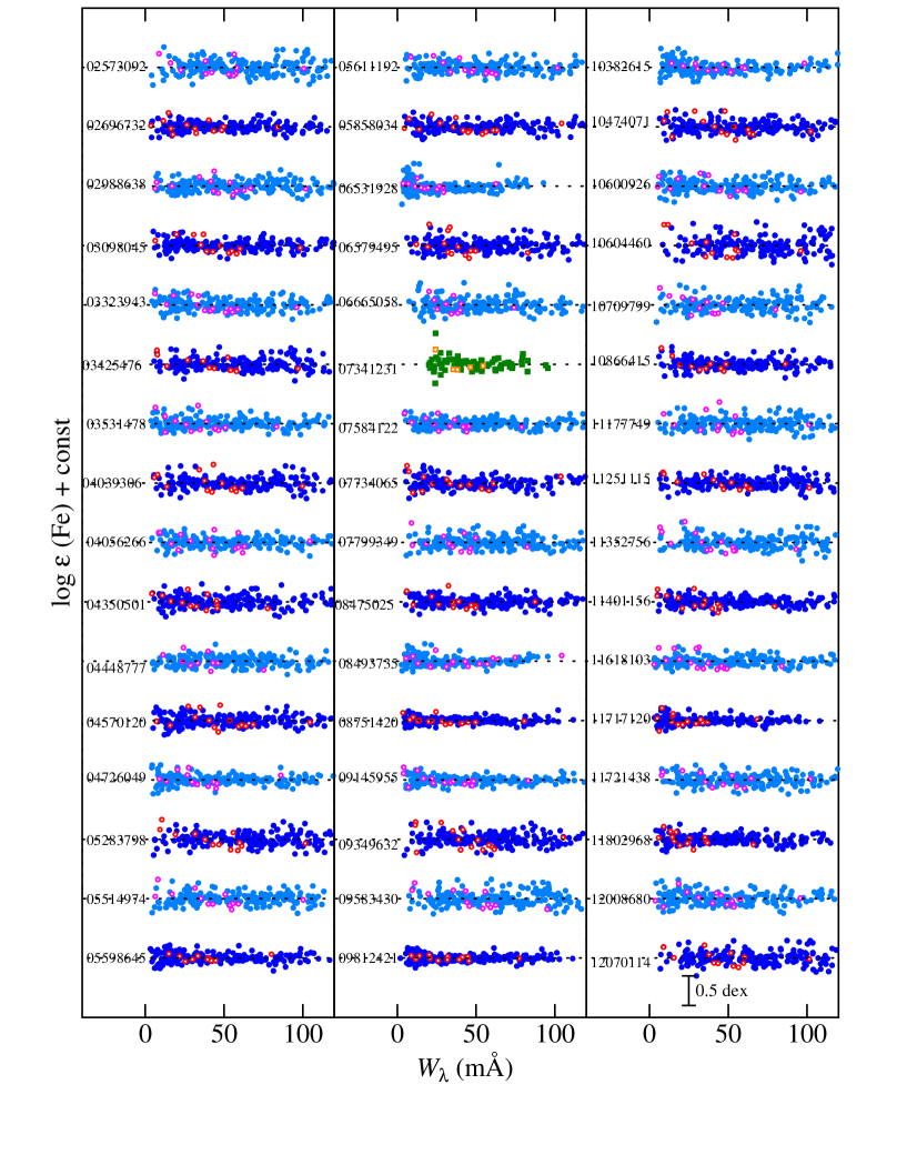
Figure 1: Fe abundance vs. equivalent width relations corresponding to the finally established atmospheric parameters of $T_{\rm eff}$, $\log g$, and $v_{\rm t}$ for each of the new 48 stars, being arranged in the increasing order of KIC number as in Table 1. The filled and open symbols correspond to Fe i and Fe ii lines, respectively. The results for each star are shown relative to the mean abundance (indicated by the horizontal dotted line), and vertically shifted by 1.0 relative to the adjacent ones. Note that a different line-set was adopted for KIC 07341231 (very metal-poor subgiant) as explained in Sect. 2.2.

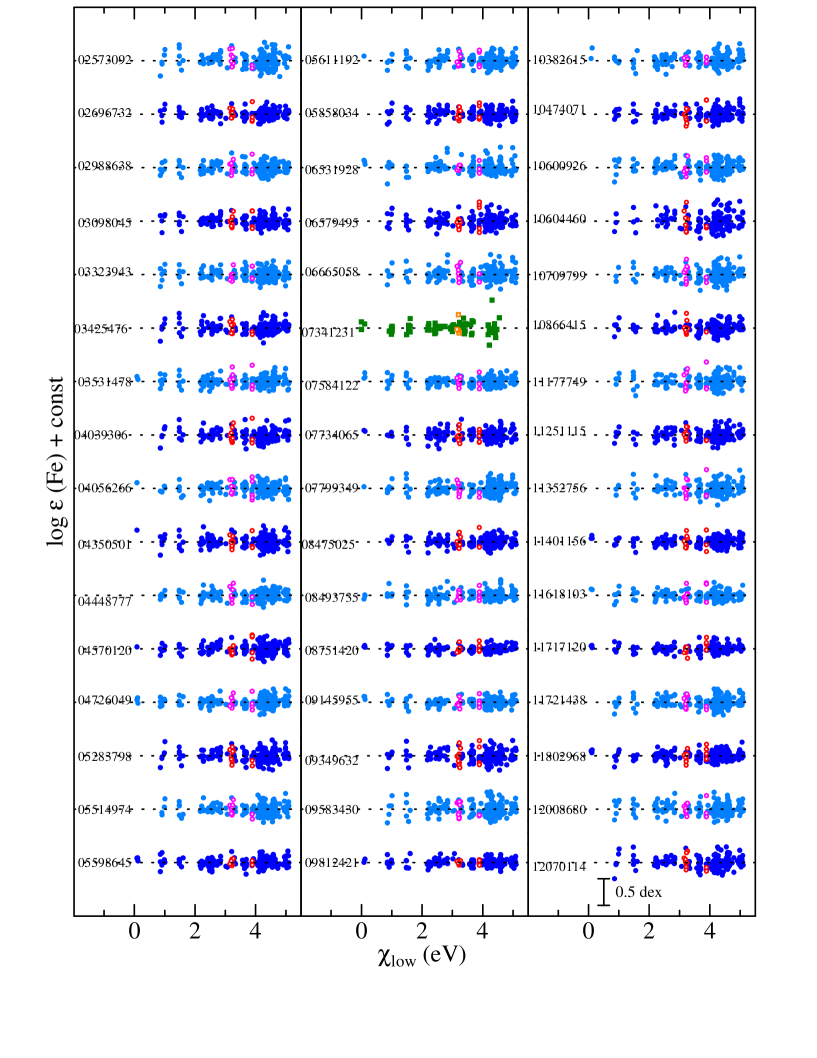
Figure 2: Fe abundance vs. lower excitation potential relations corresponding to the finally established atmospheric parameters for each of the new 48 stars. Otherwise, the same as in Fig. 1.

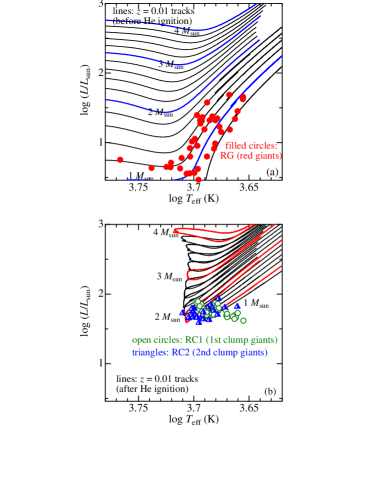
Figure 4: All the 106 program stars plotted on the $\log T_{\rm eff}$–$\log L/{\rm L}_{\odot}$ diagram. The upper panel (a) is for red giants in the shell-H-burning phase before He ignition (RG) while the lower panel (b) is for red-clump giants in the He-burning phase after He ignition (RC1 for $M<1.8$ M_⊙, RC2 for $M>1.8$ M_⊙). Symbols are discriminated according to the evolutionary status: Red filled circles $\cdots$ RG, green open circles $\cdots$ RC1, and blue triangles $\cdots$ RC2. The PARSEC tracks corresponding to each evolutionary phase (either RG tracks or RC tracks) computed for $z=0.01$ (slightly metal-deficient case by $\sim 0.2$ dex lower than the solar metallicity) and various representative mass values are overplotted for comparison.

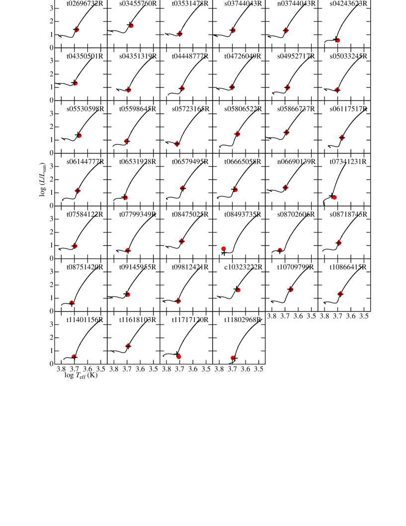
Figure 5: Comparison of the observed ($\log T_{\rm eff}$, $\log L/{\rm L}_{\odot}$) with the assigned theoretical evolutionary track for 40 RG-class stars. In each panel, the actual stellar location is indicated by a red filled circle, while the corresponding proximate point on the track is expressed by a black Greek cross. See Table 2 for the detailed data related to these figures.

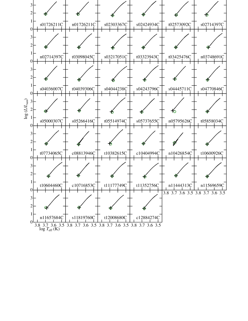
Figure 6: Comparison of the observed ($\log T_{\rm eff}$, $\log L/{\rm L}_{\odot}$) with the assigned theoretical evolutionary track for 40 RC1-class stars. In each panel, the actual stellar location is indicated by a green open circle. Otherwise, the same as in Fig. 5.

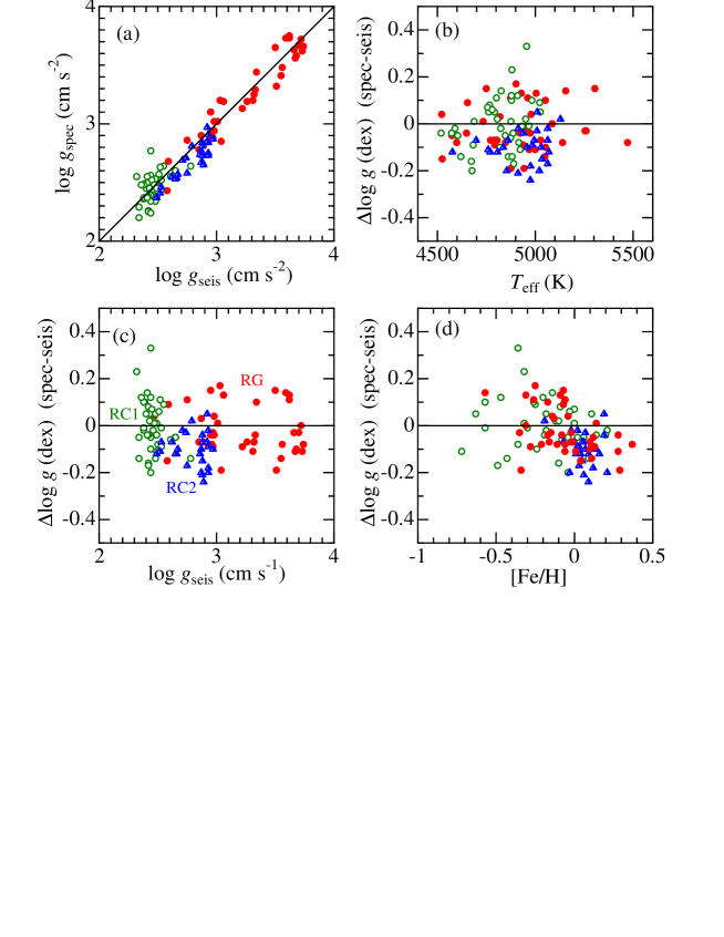
Figure 1: (a) Comparison between spectroscopic $\log g_{\rm spec}$ and seismic $\log g_{\rm seis}$ for 106 stars based the combined results of Paper I and this study. (b) Plot of the $\log g$ difference [$\Delta\log g(\equiv\log g_{\rm spec}-\log g_{\rm seis})$] against $T_{\rm eff}$. (c) Plot of $\Delta\log g$ against $\log g_{\rm seis}$. (d) $\Delta\log g$ plotted against [Fe/H]. The meanings of the symbols (discriminating the evolutionary status of RG/RC1/RC2) are the same as in Fig. 4.

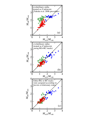
Figure 1: Comparison of asteroseismologically determined massses ($M_{\rm seis}$) for 106 Kepler giants with those estimated from evolutionary tracks ($M_{\rm trk}$), where three different kinds of tracks were tried. (a) Combined RG+RC tracks of Lejeune & Schaerer’s (2001) data were used as if the evolutionary status of each star were unknown, just as was done by Takeda et al. (2008). (b) Combined RG+RC tracks of PARSEC data (for $z_{\rm grid}$ closest to actual stellar metallicity) were used as if the evolutionary status of each star were unknown. (c) Either RG or RC tracks of PARSEC data (for $z_{\rm grid}$ closest to actual stellar metallicity) were appropriately used depending on the known evolutionary status of each star. See the caption of Fig. 4 for the meanings of the symbols.

The atmospheric parameters ($T_{\rm eff}$, $\log g$, $v_{\rm t}$, and [Fe/H]) were determined by using the measured equivalent widths of Fe i and Fe ii lines in the same way as in Paper I (see Sect. 3.1 therein). Also, the projected rotational velocity ($v_{\rm e}\sin i$) was evaluated by spectrum-fitting analysis applied to the 6080–6089 $\rm\AA$ region. The final results for these 48 Kepler giants are summarised in Table 1, where the data are arranged in the same manner as in Table 1 of Paper I. The equivalent-width data of Fe i and Fe ii lines along with the corresponding Fe abundances, and the detailed broadening/abundance results of the 6080–6089 $\rm\AA$ fitting are also presented as supplementary online material (tableE1.dat and tableE2.dat). In analogy with Paper I, Fig. 1 (Fe abundance vs. equivalent width), Fig. 2 (Fe abundance vs. excitation potential), and Fig. 3 (spectrum-fitting in 6080–6089 $\rm\AA$) are presented here (each corresponding to Fig. 4, Fig. 5, and Fig. 6 of Paper I, respectively).

2.2 Special treatment for KIC 7341231

Although the spectroscopic parameters of almost all newly observed stars were derived by exactly following the procedures of Paper I as mentioned in Sect. 2.1, only one star (KIC 7341231 = BD +42 3187) was exceptional. Actually, this is a very metal-poor ([Fe/H] = $-1.7$) subgiant of comparatively higher $T_{\rm eff}$ ($\sim 5300$ K), belonging to the halo population characterized by considerably large heliocentric radial velocity ($V_{\rm r}^{\rm hel}=-270$ km s^-1). Because of its conspicuously low metallicity along with higher $T_{\rm eff}$, the metallic lines of this star are markedly weaker compared to other giants (cf. Fig. 3), which makes it neither possible to determine the atmospheric parameters based on the adopted list of Fe i/Fe ii lines (Takeda et al. 2005), nor to accomplish a reliable fitting analysis in the 6080–6089 $\rm\AA$ region for $v_{\rm e}\sin i$ evaluation. Accordingly, we employed a different set of stronger Fe i/Fe ii lines (see “tableE1p.dat” presented as online material), which were used by Takeda et al. (2006) for their study of RR Lyr stars, in order to derive $T_{\rm eff}$, $\log g$, $v_{\rm t}$, and [Fe/H] of this star. Similarly, its $v_{\rm e}\sin i$ derivation was done by fitting in the 5200–5212 $\rm\AA$ region comprising strong lines of Cr i, Fe i, Ti i and Y i (see the inset in Fig. 3).

3 Comparison on the HR diagram

3.1 Location of each star

Our total sample consists of 106 stars (42 stars from 2014 September observation along with 16 stars from Thygesen et al.’s data as described in Paper I, and 48 stars from 2015 July observation newly presented in this paper), although the essential net number reduces to 103 because of the overlapping of 3 stars in 2014 September and Thygesen et al. samples. Since all these stars are taken from Mosser et al. (2012), their seismic radius ($R_{\rm seis}$) and mass ($M_{\rm seis}$) as well as the evolutionary stage (RG or RC1 or RC2) are already established. In addition, spectroscopically determined effective temperature ($T_{\rm eff,spec}$) and metallicity ([Fe/H]_spec) are available from our study.

In this paper, we use the term “HR diagram” indicating a plot where stellar logarithmic effective temperature [$\log T_{\rm eff}$ ($\equiv X$), where $T_{\rm eff}$ is expressed in K] and logarithmic luminosity [$\log L/{\rm L}_{\odot}$ ($\equiv Y$)] are taken as the abscissa and ordinate, respectively. We can naturally define the location of each star on this diagram, since $T_{\rm eff}$ is known and $L$ can be evaluated by the relation

$$\log(L/{\rm L}_{\odot})=4\log(T_{\rm eff,spec}/{\rm T}_{{\rm eff},\odot})+2\log(R_{\rm seis}/{\rm R}_{\odot}),$$ (1)

where quantities with $\odot$ are the reference solar values. Such determined locations in the HR diagram for all the 106 stars are plotted (separated according to whether before or after He ignition) in Fig. 4a (RG) and Fig. 4b (RC1/RC2), where representative theoretical tracks corresponding to $z=0.01$ (see the next Sect. 3.2 for more details) are also drawn for comparison.

3.2 Theoretical tracks

Our next task is to assign an appropriate theoretical track to each star in order to see whether it is consistent with the actual position. We use an extensive set of theoretical evolutionary tracks computed by the Padova–Trieste group based on their PARSEC code (Bressan et al. 2012, 2013). These tracks are provided with very fine grids in terms of $z$ (metallicity defined as the mass fraction of heavy elements) and $M$ (initial mass); i.e., $z_{\rm grid}$ = 0.06, 0.04, 0.03, 0.02, 0.017, 0.014, 0.01, 0.008, 0.006, 0.004, 0.002, 0.001, 0.0005, 0.0002, and 0.0001, while the mesh of $M_{\rm grid}$ is 0.05 M_⊙ step (for 1–2.3 M_⊙) or 0.1 M_⊙ step (for 2.3–5 M_⊙). Since these parameter grids are sufficiently fine, we assign to each star the track corresponding to ($z_{\rm grid}$, $M_{\rm grid}$) being nearest to the actual ($z_{\rm star}$, $M_{\rm star}$), where $M_{\rm star}\equiv M_{\rm seis}$ and $z_{\rm star}\equiv 0.014\times 10^{\rm[Fe/H]_{spec}}$ (z${}_{\odot}=0.014$ is the solar value; cf. Asplund et al. 2009). The actual ($z_{\rm star}$, $M_{\rm star}$) as well as the adopted ($z_{\rm grid}$, $M_{\rm grid}$) for each star are presented in Table 2. Since the evolutionary stage is known for all the targets, we naturally allocate “RG tracks” (track portion from the point of “end of core H-burning” through the point of “He ignition”) to RG-class stars, and “RC tracks” (track portion from the point of “He ignition” through the point of “asymptotic giant branch tip”) to RC1/RC2-class stars.

3.3 Matching check

Comparison of the position on the HR diagram with the assigned track for each star is graphically depicted in Fig. 5 (RG stars), Fig. 6 (RC1 stars), and Fig. 7 (RC2 stars). We indicate in each panel the “proximate point” ($X^{*}_{\rm track}$, $Y^{*}_{\rm track}$) on the track by a Greek cross, where the distance-measure $d^{2}(t)$ ($t$ is the age variable of a track) defined by

$$d^{2}(t)\equiv[(10X_{\rm star}-10X_{\rm track}(t)]^{2}+[(Y_{\rm star}-Y_{\rm track}(t)]^{2}$$ (2)

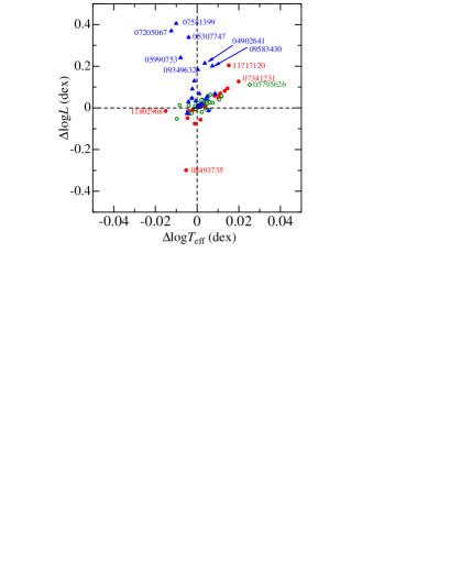
Figure 8: $\Delta\log L$ vs. $\Delta\log T_{\rm eff}$ (or $\Delta Y$ vs. $\Delta X$) plot based on the data given in Table 2, showing the behavior of theory$-$observation difference in the HR diagram for each star. The meanings of the symbols are the same as in Fig. 4. Stars showing rather large discrepancies are indicated in the figure.

becomes minimum. These figures suggest that the agreement between ($X_{\rm star}$, $Y_{\rm star}$) and ($X^{*}_{\rm track}$, $Y^{*}_{\rm track}$) is satisfactory in most cases, though appreciably discrepant cases sometimes show up (e.g., in RG and RC2 classes). In order to clarify this situation quantitatively, the coordinate differences between the two points ($\Delta X\equiv X^{*}_{\rm track}-X_{\rm star}$, $\Delta Y\equiv Y^{*}_{\rm track}-Y_{\rm star}$) were computed (cf. Table 2) and the $\Delta Y$ vs. $\Delta X$ plot is displayed in Fig. 8, from which the following consequences can be extracted.
— Generally, a reasonable consistency to a level of $\Delta X\la 0.01$ dex (i.e., $\Delta T_{\rm eff}\la 100$ K) and $\Delta Y\la 0.1$ dex (i.e., $\la 0.2$ mag in magnitude) is accomplished for a majority ($\sim$ 90%) of our targets, indicating reasonable reliability of recent stellar evolution calculations in the sense that theoretical tracks can satisfactorily reproduce the observed positions of red giant stars on the HR diagram.
— However, appreciable discrepancies are sometimes seen especially in a group of RC2 stars (e.g., KIC 07581399, 07205067, 05307747, 05990753, 04902641, 09583430, 09349632), the observed lumonosities of which are by $\sim$ 0.2–0.4 dex lower than the theoretically predicted red-clump luminosities (cf. the corresponding panels in Fig. 7). A closer inspection in reference to Table 2 revealed that these stars have apparently higher mass values (2.5 ${\rm M}_{\odot}\la M\la$ 3.5 ${\rm M}_{\odot}$) even among RC2 stars (RC stars of $M>1.8$ ${\rm M}_{\odot}$). Actually, we can recognize from Fig. 4b that the luminosities of all RC2 stars (tiangles) tightly cluster at $\log(L/{\rm L}_{\odot})\sim$ 1.6–1.9 almost irrespective of their masses (1.8 ${\rm M}_{\odot}\la M\la$ 3.5 ${\rm M}_{\odot}$), which apparently contradicts the theoretical RC2 tracks ($\log L$ increases by $\sim 0.5$ dex for a mass change from $\sim 2$ ${\rm M}_{\odot}$ to $\sim 3$ ${\rm M}_{\odot}$). We can not find any reasonable explanation for this inconsistency seen in higher-mass RC2 stars; it may be worthwhile to reexamine whether their assigned evolutionary tracks as well as $M$ and/or $R$ determination procedures are really valid.
— Regarding RC1 and RG stars, the agreement is satisfactory in most cases, excepting that appreciable differences are seen in several stars; e.g., KIC 05795626 for RC1, KIC 11717120, 07341231, and 08493735 for RG (note that these RG stars are not so much on the ascending track of red-giants as rather subgiants). We also notice a tendency of weak (positive) correlation between $\Delta\log L$ and $\Delta\log T_{\rm eff}$ (cf. Fig. 8).

4 Age–metallicity relation of giants

4.1 Derivation of age

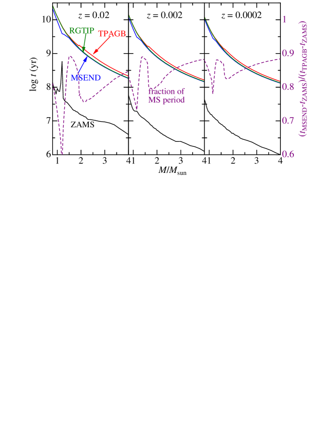
Figure 9: Elapsed times (measured from the beginning of star formation; expressed in logarithmic scale in unit of yr) of PARSEC stellar evolutionary tracks at four critical phases are plotted against the stellar mass. Black line, blue line, green line, and red line correspond to (i) zero-age main-sequence (ZAMS), (ii) main-sequence end (MSEND), (iii) red-giant tip at He-ignition (RGTIP), and (iv) beginning of thermally-pulsing asymptotic giant-branch (TPAGB), respectively. The fraction of main-sequence period, which is defined as $(t_{\rm MSEND}-t_{\rm ZAMS})/(t_{\rm TPAGB}-t_{\rm ZAMS})$, is also shown in purple dashed lines (its scale is given at the rightmost ordinate). Each panel displays results for models of different metallicity: $z=0.02$ (left), $z=0.002$ (middle), and $z=0.0002$ (right).

As a natural by-product of determining the proximate point on the track ($X^{*}_{\rm track}$, $Y^{*}_{\rm track}$) described in Sect. 3.3, we can derive the stellar age as the corresponding $t$ value ($t^{*}$). Note, however, that the age is mainly determined by the stellar mass in the present case of giant stars (see, e.g., Fig. 3c in Takeda et al. 2008), since it restricts the predominantly long lifetime on the main sequence, compared to which the period of post-main-sequence phase is insignificant. So, pinpointing the location on the giant track is not necessarily very important in this respect. In order to clarify this situation, the elapsed times at the track points of several critical evolutionary phases as well as the corresponding fraction of main-sequence period are plotted against the stellar mass in Fig. 9, where we can see that these giants have spent a major fraction ($\sim$ 60–90%) of their past life on the main sequence.

In order to maintain the consistency with the previous work, we define “$age$” as the time elapsed from the zero-age main sequence (ZAMS) as $age\equiv t^{*}-t({\rm ZAMS})$. Such derived $age$ values are given in Table 2.

4.2 Result and implication

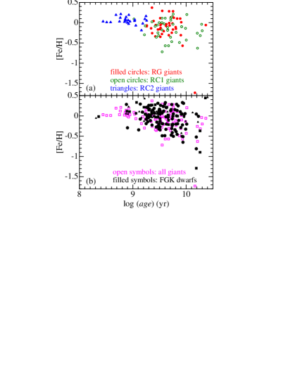
Figure 10: (a) Metallicity ([Fe/H]) vs. $age$ ($\equiv t-t_{\rm ZAMS}$) relation derived for 106 Kepler giants, where stars for each evolutionary phases are discriminated by symbols as in Fig. 4. (b) Comparison of the [Fe/H] vs. $age$ relation of 106 Kepler giants (pink open squares) with that of 160 FGK dwarfs (black filled symbols) derived by Takeda (2007). In the latter diagram, reliability classes (see Sect. 2 of Takeda 2007) are discriminated by its type and size. (A: reliable) $\cdots$ large circles, (B: less reliable) $\cdots$ medium-size squares, (C: unreliable) $\cdots$ small triangles.

The resulting $age$ vs. [Fe/H] distribution for our 106 Kepler giants is depicted in Fig. 10a, and the comparison with the relation derived for field FGK dwarfs (Takeda 2007) is shown in Fig. 10b. We can recognize from Fig. 10b that both results of giants and dwarfs are quite consistent with each other, without any systematic discrepancy such as that Takeda et al. (2008) once claimed (which is evidently due to erroneous overestimation of mass for many giants as pointed out in Paper I).

Regarding the observational study of galactic age–metallicity relation, not a few papers have been published so far (see, e.g., Sect. 1 of Bergemann et al. 2014 and the references therein). Although any consensus has not yet been accomplished concerning the detailed characteristics, it is no doubt that the metallicity at a given age is by no means single-valued but more or less diversified. Our result implies that the [Fe/H] dispersion tends to progressively increase with $age$ (from several $\times 10^{8}$ yr to $\sim 10^{10}$ yr) while the maximum metallicity does not change much (i.e., near/super-solar level is retained over this large span of $age$), resulting in a “right triangle-like” shape.

Especially, the existence of very old ($age$ $\sim 10^{10}$ yr) metal-rich ($0.0\la$ [Fe/H] $\la 0.4$) stars may be regarded as a significant consequence. How should we interpret their origin? Were they born in the galactic bulge and migrated to the present position over the long passage of time? From this point of view, it would be interesting and worthwhile to study the chemical abundances of key elements (e.g., $\alpha$-group) of these old stars of high metallicity and to compare them with those of younger meta-rich stars.

5 Summary and conclusion

Recent very high-precision photometric observations from satellites have enabled discrimination of the evolutionary status (RG/RC1/RC2) as well as determinations of $M$ and $R$ for a large number of red giant stars by exploiting the asteroseimological technique.

Following the same manner in Paper I where our first pilot study was done for 58 stars, we determined in this study the atmospheric parameters ($T_{\rm eff}$, $\log g$, $v_{\rm t}$, and [Fe/H]) for additional 48 giants in the Kepler field by using Fe i and Fe ii lines.

Given that spectroscopic and seismic information is now available for these 106 red giants in total, we could readily define the position on the $\log L$ vs. $\log T_{\rm eff}$ diagram and to assign an appropriate theoretical evolutionary track to each star.

Our first aim was to examine whether the observed stellar location on this diagram really matches the assigned theoretical track. We could confirm that the assigned track is mostly consistent with the actual position (to a level of $\la 100$ K in $T_{\rm eff}$ and $\la 0.2$ mag in $M_{\rm bol}$) for a majority ($\sim 90$%) of our targets. Accordingly, we may state that recent stellar evolution calculations are reasonably reliable.

However, appreciable inconsistencies are seen for $\sim 10$% of the sample stars. Especially noteworthy is that the luminosities of several RC2 stars with higher-$M$ (2.5 ${\rm M}_{\odot}\la M\la$ 3.5 ${\rm M}_{\odot}$) do not agree with the corresponding theorerical tracks, because they tend to tightly cluster at $\log(L/{\rm L}_{\odot})\sim$ 1.6–1.9 irrespective of their masses, which apparently contradicts the theoretical prediction. It may be worthwhile to reexamine the validity of assigned evolutionary tracks and of the $M$ as well as $R$ values for these stars.

Our second purpose was to establish the age–metallicity relation based on these giant stars, since the stellar age could be as a natural by-product of location–track comparison on the HR diagram. The resulting distribution for giants turned out to be in good agreement with that for FGK dwarfs derived by Takeda (2007), which is characterized by growing metallicity dispersion with an increase in age while the maximum metallicity remains almost flat at the near/super-solar level over the wide age range from $\sim$ (2–3) $\times 10^{8}$ yr to $\sim 10^{10}$ yr.

The fact that very old ($age$ $\sim 10^{10}$ yr) metal-rich ($0.0\la$ [Fe/H] $\la 0.4$) stars do exist may be regarded as a significant consequence from the viewpoint of galactic chemical evolution. Studying the chemical abundance characteristics of these stars in detail would be worthwhile toward clarifying their origin.

Table 1: Basic data and the resulting parameters of the newly observed 48 stars.

KIC#	$Kepler$	$T_{\rm eff}$	$\log g$	$v_{\rm t}$	[Fe/H]	$\nu_{\rm max}$	$\Delta\nu$	$\Delta\Pi_{1}$	$R_{\rm seis}$	$M_{\rm seis}$	$\log g_{\rm seis}$	$v_{\rm e}\sin i$	class
(1)	(2)	(3)	(4)	(5)	(6)	(7)	(8)	(9)	(10)	(11)	(12)	(13)	(14)
02573092	11.58	4689	2.48	1.38	+0.00	35.9	4.08	293.80	11.60	1.43	2.47	2.1	RC1
02696732	11.50	4821	2.90	1.04	$-$0.13	90.4	8.39	66.55	7.01	1.33	2.87	1.9	RG
02988638	12.16	4912	2.67	1.22	+0.06	91.4	7.42	178.12	9.14	2.31	2.88	2.2	RC2
03098045	11.83	4820	2.34	1.29	$-$0.24	33.3	4.15	281.10	10.54	1.11	2.44	2.1	RC1
03323943	11.61	4826	2.55	1.26	$-$0.14	31.0	4.03	286.02	10.41	1.01	2.41	2.1	RC1
03425476	11.68	4780	2.57	1.30	$-$0.03	39.0	4.42	303.60	10.84	1.37	2.51	2.2	RC1
03531478	11.64	5000	3.20	0.98	$-$0.06	243.5	17.35	87.60	4.49	1.50	3.31	1.8	RG
04039306	11.55	4806	2.45	1.30	$-$0.10	32.5	4.15	312.20	10.27	1.03	2.43	2.2	RC1
04056266	11.78	5021	2.67	1.17	$-$0.03	89.0	7.38	270.80	9.09	2.25	2.87	2.1	RC2
04350501	11.74	4929	3.19	1.01	$-$0.09	139.0	11.10	69.30	6.22	1.63	3.06	2.0	RG
04448777	11.56	4805	3.19	0.95	+0.10	220.4	17.02	89.90	4.14	1.13	3.26	1.5	RG
04570120	11.64	5035	2.73	1.20	+0.05	90.8	7.35	277.10	9.37	2.44	2.88	2.6	RC2
04726049	11.83	5029	3.25	0.97	$-$0.16	248.0	18.03	89.40	4.25	1.37	3.32	1.8	RG
05283798	11.71	4770	2.53	1.30	+0.09	54.8	5.33	268.98	10.46	1.79	2.65	2.2	RC2
05514974	11.36	4674	2.26	1.30	$-$0.10	32.2	4.07	327.10	10.44	1.03	2.42	2.0	RC1
05598645	11.69	5052	3.44	0.86	$-$0.17	260.1	19.59	91.18	3.78	1.14	3.34	2.0	RG
05611192	11.82	5064	2.91	1.20	+0.02	101.1	7.99	216.70	8.85	2.43	2.93	3.0	RC2
05858034	11.74	4887	2.45	1.28	$-$0.19	37.6	4.42	268.60	10.56	1.27	2.49	2.1	RC1
06531928	10.70	5156	3.73	0.69	$-$0.57	458.2	31.58	115.80	2.59	0.95	3.59	2.0	RG
06579495	11.86	4772	2.78	1.03	$-$0.02	85.6	8.19	73.80	6.92	1.22	2.85	1.2	RG
06665058	11.49	4750	3.10	0.86	$-$0.07	107.6	9.79	77.40	6.08	1.18	2.95	2.0	RG
07341231	9.91	5305	3.65	1.31	$-$1.73	368.0	28.95	112.75	2.51	0.73	3.50	1.2	RG
07584122	11.69	4974	3.29	0.93	$-$0.08	252.4	18.57	91.66	4.05	1.26	3.33	1.9	RG
07734065	11.71	4882	2.20	1.28	$-$0.43	26.6	3.68	318.40	10.78	0.93	2.34	1.9	RC1
07799349	9.47	4969	3.56	0.94	+0.28	562.7	33.53	109.80	2.77	1.31	3.67	2.1	RG
08475025	11.71	4848	2.88	1.02	$-$0.06	110.9	9.66	74.80	6.50	1.41	2.96	1.9	RG
08493735	10.07	5842	3.62	1.14	+0.01	586.1	38.86	113.12	2.33	1.05	3.73	3.9	RG
08751420	6.91	5260	3.63	0.95	$-$0.15	536.4	34.70	135.40	2.54	1.08	3.66	2.1	RG
09145955	9.78	4943	2.85	1.05	$-$0.34	130.0	11.00	77.01	5.93	1.39	3.04	1.7	RG
09349632	11.85	4976	2.75	1.12	+0.12	100.8	7.79	226.80	9.20	2.60	2.93	2.6	RC2
09583430	11.60	4854	2.73	1.19	+0.21	102.2	7.78	166.30	9.24	2.62	2.93	2.2	RC2
09812421	10.19	5140	3.48	0.87	$-$0.21	427.5	27.85	112.00	3.10	1.27	3.56	2.0	RG
10382615	11.68	4890	2.25	1.27	$-$0.49	31.6	4.12	301.01	10.22	1.00	2.42	2.4	RC1
10474071	11.70	4975	2.65	1.17	+0.09	93.1	7.50	266.80	9.17	2.38	2.89	2.1	RC2
10600926	11.64	4879	2.48	1.29	$-$0.20	27.7	3.91	329.40	9.94	0.82	2.36	2.3	RC1
10604460	10.92	4573	2.37	1.30	+0.14	31.7	3.80	308.30	11.66	1.26	2.41	3.6	RC1
10709799	10.82	4522	2.51	1.11	$-$0.04	36.9	4.21	57.20	10.99	1.29	2.47	1.7	RG
10866415	11.02	4791	2.82	0.93	$-$0.01	94.4	8.78	67.70	6.66	1.25	2.89	2.0	RG
11177749	10.90	4677	2.24	1.26	$-$0.04	33.6	4.05	304.00	11.00	1.20	2.44	2.0	RC1
11251115	7.88	4837	2.57	1.29	+0.07	56.7	5.08	295.20	12.00	2.45	2.67	2.2	RC2
11352756	10.96	4604	2.29	1.31	$-$0.04	27.0	3.71	300.30	10.45	0.86	2.34	2.3	RC1
11401156	9.89	5053	3.58	0.90	+0.10	571.0	35.78	115.00	2.49	1.09	3.68	1.8	RG
11618103	7.70	4922	2.91	1.10	$-$0.17	106.0	9.38	74.40	6.64	1.41	2.95	1.6	RG
11717120	9.27	5087	3.72	0.75	$-$0.31	623.2	37.80	130.50	2.44	1.14	3.72	1.7	RG
11721438	11.75	4959	2.87	1.12	+0.14	111.0	8.53	177.60	8.44	2.40	2.97	2.4	RC2
11802968	10.89	4962	3.73	0.75	$-$0.06	498.9	34.50	116.10	2.32	0.81	3.62	1.5	RG
12008680	11.21	4881	2.55	1.31	$-$0.32	25.1	3.65	321.80	10.34	0.81	2.32	2.7	RC1
12070114	10.86	4698	2.46	1.30	+0.05	41.2	4.28	237.70	12.10	1.78	2.53	2.1	RC2

The data of these new 48 stars are arranged in the same manner as in Table 1 of Paper I. Following the serial number and the $Kepler$ magnitude (in mag) of the Kepler Input Catalogue (KIC; cf. Brown et al. 2011) in Columns (1) and (2), the atmospheric parameters (effective temperature $T_{\rm eff}$ in K, logarithmic surface gravity $\log g$ in cm s^-2/dex, microturbulent velocity dispersion $v_{\rm t}$ in km s^-1, and metallicity [Fe/H] in dex) spectroscopically determined from Fe i and Fe ii lines are presented in Columns (3)–(6). Columns (7)–(9) give the asteroseismic quantities taken from Mosser et al. (2012): the central frequency of the oscillation power excess ($\nu_{\rm max}$ in $\mu$Hz), the large frequency separation ($\Delta\nu$ in $\mu$Hz), and the gravity-mode spacing ($\Delta\Pi_{1}$ in unit of s; good indicator for discriminating between RG and RC1/RC2). Presented in Columns (10)–(12) are the seismic radius (in R_⊙), seismic mass (in M_⊙), and the corresponding seismic surface gravity (in cm s^-2/dex), which were evaluated from $\nu_{\rm max}$ and $\Delta\nu$ by using the scaling relations as in Paper I. In Columns (13) and (14) are given the projected rotational velocity (in km s^-1; derived from spectrum-fitting analysis) and the evolutionary class determined by Mosser et al. (2012) (RG: red giant, RC1: 1st clump giant, RC2: 2nd clump giant).

Table 2: Matching results between stellar positions on the HR diagram and assigned evolutionary tracks.

star code	[Fe/H]	$z_{\rm star}$	$z_{\rm grid}$	$M_{\rm star}$	$M_{\rm grid}$	$X_{\rm star}$	$Y_{\rm star}$	$\Delta X$	$\Delta Y$	$\log age$	Figure
(1)	(2)	(3)	(4)	(5)	(6)	(7)	(8)	(9)	(10)	(11)	(12)
[RG-class stars]
t02696732R	$-$0.13	0.0104	0.0100	1.33	1.35	3.6831	1.376	+0.0037	+0.020	9.521	Fig.5(1,1)
s03455760R	$-$0.07	0.0119	0.0100	1.63	1.65	3.6678	1.686	+0.0111	+0.070	9.263	Fig.5(1,2)
t03531478R	$-$0.06	0.0122	0.0140	1.50	1.50	3.6990	1.053	+0.0022	+0.019	9.429	Fig.5(1,3)
s03744043R	$-$0.35	0.0063	0.0060	1.31	1.30	3.6943	1.321	+0.0058	+0.028	9.516	Fig.5(1,4)
n03744043R	$-$0.28	0.0073	0.0080	1.31	1.30	3.6936	1.317	+0.0006	+0.004	9.545	Fig.5(1,5)
s04243623R	$-$0.31	0.0069	0.0060	0.99	1.00	3.6994	0.566	+0.0146	+0.094	9.900	Fig.5(1,6)
t04350501R	$-$0.09	0.0114	0.0100	1.63	1.65	3.6928	1.311	+0.0089	+0.060	9.260	Fig.5(2,1)
s04351319R	+0.29	0.0273	0.0300	1.45	1.45	3.6881	0.800	+0.0044	+0.031	9.552	Fig.5(2,2)
t04448777R	+0.10	0.0176	0.0170	1.13	1.15	3.6817	0.913	+0.0040	+0.009	9.830	Fig.5(2,3)
t04726049R	$-$0.16	0.0097	0.0100	1.37	1.35	3.7015	1.015	+0.0018	+0.006	9.509	Fig.5(2,4)
s04952717R	+0.13	0.0189	0.0200	1.24	1.25	3.6806	0.987	+0.0026	+0.011	9.713	Fig.5(2,5)
s05033245R	+0.11	0.0180	0.0170	1.41	1.40	3.7032	0.800	$-$0.0009	$-$0.008	9.513	Fig.5(2,6)
s05530598R	+0.37	0.0328	0.0300	1.68	1.67	3.6627	1.340	+0.0108	+0.061	9.359	Fig.5(3,1)
t05598645R	$-$0.17	0.0095	0.0100	1.14	1.15	3.7035	0.921	$-$0.0044	$-$0.016	9.752	Fig.5(3,2)
s05723165R	$-$0.02	0.0134	0.0140	1.36	1.35	3.7206	0.710	$-$0.0005	+0.004	9.541	Fig.5(3,3)
s05806522R	+0.12	0.0185	0.0170	1.18	1.20	3.6603	1.451	+0.0034	+0.018	9.768	Fig.5(3,4)
s05866737R	$-$0.26	0.0077	0.0080	1.52	1.50	3.6879	1.577	+0.0014	+0.005	9.363	Fig.5(3,5)
s06117517R	+0.28	0.0267	0.0300	1.26	1.25	3.6674	1.187	$-$0.0008	$-$0.003	9.754	Fig.5(3,6)
s06144777R	+0.14	0.0193	0.0200	1.18	1.20	3.6752	1.153	+0.0000	+0.000	9.745	Fig.5(4,1)
t06531928R	$-$0.57	0.0038	0.0040	0.95	0.95	3.7123	0.628	+0.0084	+0.059	9.932	Fig.5(4,2)
t06579495R	$-$0.02	0.0134	0.0140	1.22	1.20	3.6787	1.347	$-$0.0033	$-$0.016	9.743	Fig.5(4,3)
t06665058R	$-$0.07	0.0119	0.0100	1.18	1.20	3.6767	1.227	+0.0102	+0.045	9.689	Fig.5(4,4)
n06690139R	$-$0.14	0.0101	0.0100	1.56	1.55	3.6971	1.396	$-$0.0010	$-$0.005	9.343	Fig.5(4,5)
t07341231R	$-$1.73	0.0003	0.0002	0.73	0.75	3.7247	0.650	+0.0199	+0.127	10.164	Fig.5(4,6)
t07584122R	$-$0.08	0.0116	0.0100	1.26	1.25	3.6967	0.954	+0.0042	+0.017	9.622	Fig.5(5,1)
t07799349R	+0.28	0.0267	0.0300	1.31	1.30	3.6963	0.622	$-$0.0039	$-$0.027	9.679	Fig.5(5,2)
t08475025R	$-$0.06	0.0122	0.0140	1.41	1.40	3.6856	1.320	$-$0.0012	$-$0.006	9.519	Fig.5(5,3)
t08493735R	+0.01	0.0143	0.0140	1.05	1.05	3.7666	0.753	$-$0.0053	$-$0.299	9.908	Fig.5(5,4)
s08702606R	$-$0.11	0.0109	0.0100	1.09	1.10	3.7381	0.636	+0.0016	$-$0.057	9.803	Fig.5(5,5)
s08718745R	$-$0.25	0.0079	0.0080	1.17	1.15	3.6904	1.190	+0.0033	+0.011	9.730	Fig.5(5,6)
t08751420R	$-$0.15	0.0099	0.0100	1.08	1.10	3.7210	0.646	$-$0.0011	$-$0.075	9.808	Fig.5(6,1)
t09145955R	$-$0.34	0.0064	0.0060	1.39	1.40	3.6940	1.274	+0.0117	+0.055	9.423	Fig.5(6,2)
t09812421R	$-$0.21	0.0086	0.0080	1.27	1.25	3.7110	0.779	+0.0036	+0.024	9.580	Fig.5(6,3)
c10323222R	+0.04	0.0154	0.0140	1.55	1.55	3.6556	1.624	+0.0133	+0.082	9.390	Fig.5(6,4)
t10709799R	$-$0.04	0.0128	0.0140	1.29	1.30	3.6553	1.656	+0.0051	+0.032	9.630	Fig.5(6,5)
t10866415R	$-$0.01	0.0137	0.0140	1.25	1.25	3.6804	1.321	$-$0.0021	$-$0.011	9.682	Fig.5(6,6)
t11401156R	+0.10	0.0176	0.0170	1.09	1.10	3.7035	0.559	$-$0.0046	$-$0.049	9.888	Fig.5(7,1)
t11618103R	$-$0.17	0.0095	0.0100	1.41	1.40	3.6921	1.365	$-$0.0013	$-$0.006	9.471	Fig.5(7,2)
t11717120R	$-$0.31	0.0069	0.0060	1.14	1.15	3.7065	0.553	+0.0152	+0.204	9.675	Fig.5(7,3)
t11802968R	$-$0.06	0.0122	0.0140	0.81	0.80	3.6957	0.466	$-$0.0151	$-$0.015	10.368	Fig.5(7,4)
[RC1-class stars]
s01726211C	$-$0.57	0.0038	0.0040	1.19	1.20	3.6975	1.873	+0.0028	+0.033	9.608	Fig.6(1,1)
n01726211C	$-$0.57	0.0038	0.0040	1.17	1.15	3.6931	1.851	+0.0052	+0.057	9.670	Fig.6(1,2)
s02303367C	+0.06	0.0161	0.0170	1.23	1.25	3.6629	1.695	+0.0052	+0.037	9.712	Fig.6(1,3)
s02424934C	$-$0.18	0.0092	0.0100	1.36	1.35	3.6805	1.813	+0.0019	+0.017	9.547	Fig.6(1,4)
t02573092C	+0.00	0.0140	0.0140	1.43	1.45	3.6711	1.766	+0.0060	$-$0.009	9.495	Fig.6(1,5)
s02714397C	$-$0.47	0.0047	0.0040	1.12	1.10	3.6911	1.766	+0.0105	+0.040	9.729	Fig.6(1,6)
n02714397C	$-$0.36	0.0061	0.0060	1.14	1.15	3.6951	1.787	+0.0000	+0.002	9.708	Fig.6(2,1)
t03098045C	$-$0.24	0.0081	0.0080	1.11	1.10	3.6830	1.730	+0.0023	+0.019	9.811	Fig.6(2,2)
s03217051C	+0.21	0.0227	0.0200	1.22	1.20	3.6618	1.662	+0.0025	+0.040	9.758	Fig.6(2,3)
t03323943C	$-$0.14	0.0101	0.0100	1.01	1.00	3.6836	1.722	$-$0.0008	$-$0.005	9.988	Fig.6(2,4)
t03425476C	$-$0.03	0.0131	0.0140	1.37	1.35	3.6794	1.740	$-$0.0010	+0.009	9.589	Fig.6(2,5)
n03748691C	+0.11	0.0180	0.0170	1.37	1.35	3.6778	1.758	$-$0.0039	$-$0.020	9.607	Fig.6(2,6)
s04036007C	$-$0.36	0.0061	0.0060	1.38	1.40	3.6916	1.798	+0.0048	+0.021	9.441	Fig.6(3,1)
t04039306C	$-$0.10	0.0111	0.0100	1.03	1.05	3.6818	1.703	+0.0005	+0.024	9.915	Fig.6(3,2)
s04044238C	+0.20	0.0222	0.0200	1.06	1.05	3.6550	1.616	+0.0063	+0.064	10.012	Fig.6(3,3)
s04243796C	+0.11	0.0180	0.0170	1.26	1.25	3.6646	1.676	+0.0044	+0.043	9.712	Fig.6(3,4)
s04445711C	$-$0.32	0.0067	0.0060	1.35	1.35	3.6881	1.789	+0.0075	+0.025	9.484	Fig.6(3,5)
s04770846C	+0.02	0.0147	0.0140	1.58	1.60	3.6855	1.684	$-$0.0026	+0.047	9.359	Fig.6(3,6)
s05000307C	$-$0.25	0.0079	0.0080	1.41	1.40	3.7010	1.794	$-$0.0083	+0.013	9.470	Fig.6(4,1)
s05266416C	$-$0.09	0.0114	0.0100	1.51	1.50	3.6782	1.858	+0.0032	+0.029	9.418	Fig.6(4,2)
t05514974C	$-$0.10	0.0111	0.0100	1.03	1.05	3.6697	1.668	+0.0086	+0.067	9.913	Fig.6(4,3)
s05737655C	$-$0.63	0.0033	0.0040	0.78	0.80	3.7012	1.688	+0.0045	+0.032	10.213	Fig.6(4,4)
n05795626C	$-$0.72	0.0027	0.0020	1.21	1.20	3.6922	1.751	+0.0253	+0.111	9.549	Fig.6(4,5)
t05858034C	$-$0.19	0.0090	0.0100	1.27	1.25	3.6890	1.756	$-$0.0040	+0.011	9.651	Fig.6(4,6)
t07734065C	$-$0.43	0.0052	0.0060	0.93	0.95	3.6886	1.772	+0.0022	$-$0.020	10.001	Fig.6(5,1)
c08813946C	+0.09	0.0172	0.0170	2.09	2.10	3.6868	1.678	+0.0014	+0.004	9.022	Fig.6(5,2)
t10382615C	$-$0.49	0.0045	0.0040	1.00	1.00	3.6893	1.728	+0.0118	+0.058	9.873	Fig.6(5,3)
c10404994C	$-$0.06	0.0122	0.0140	1.50	1.50	3.6815	1.774	$-$0.0004	$-$0.002	9.459	Fig.6(5,4)
n10426854C	$-$0.30	0.0070	0.0080	1.78	1.80	3.6962	1.892	$-$0.0034	$-$0.027	9.218	Fig.6(5,5)
t10600926C	$-$0.20	0.0088	0.0080	0.82	0.80	3.6883	1.700	+0.0005	+0.006	10.300	Fig.6(5,6)

Table 2: (Continued.)

star code	[Fe/H]	$z_{\rm star}$	$z_{\rm grid}$	$M_{\rm star}$	$M_{\rm grid}$	$X_{\rm star}$	$Y_{\rm star}$	$\Delta X$	$\Delta Y$	$\log age$	Figure
(1)	(2)	(3)	(4)	(5)	(6)	(7)	(8)	(9)	(10)	(11)	(12)
[RC1-class stars]
t10604460C	+0.14	0.0193	0.0200	1.26	1.25	3.6602	1.726	+0.0039	$-$0.004	9.731	Fig.6(6,1)
c10716853C	$-$0.08	0.0116	0.0100	1.75	1.75	3.6879	1.780	+0.0049	+0.047	9.233	Fig.6(6,2)
t11177749C	$-$0.04	0.0128	0.0140	1.20	1.20	3.6700	1.715	+0.0023	+0.018	9.753	Fig.6(6,3)
t11352756C	$-$0.04	0.0128	0.0140	0.86	0.85	3.6631	1.643	+0.0060	+0.026	10.290	Fig.6(6,4)
n11444313C	+0.00	0.0140	0.0140	1.39	1.40	3.6773	1.797	$-$0.0005	$-$0.005	9.547	Fig.6(6,5)
n11569659C	$-$0.26	0.0077	0.0080	0.85	0.85	3.6883	1.689	+0.0001	+0.003	10.209	Fig.6(6,6)
n11657684C	$-$0.12	0.0106	0.0100	1.27	1.25	3.6947	1.824	$-$0.0097	$-$0.052	9.652	Fig.6(7,1)
s11819760C	$-$0.18	0.0092	0.0100	1.25	1.25	3.6834	1.843	$-$0.0026	$-$0.026	9.654	Fig.6(7,2)
t12008680C	$-$0.32	0.0067	0.0060	0.81	0.80	3.6885	1.735	+0.0029	+0.035	10.264	Fig.6(7,3)
c12884274C	+0.11	0.0180	0.0170	1.39	1.40	3.6705	1.689	+0.0021	+0.038	9.548	Fig.6(7,4)
[RC2-class stars]
s02013502S	$-$0.02	0.0134	0.0140	1.94	1.95	3.6913	1.740	+0.0013	+0.014	9.187	Fig.7(1,1)
s02448225S	+0.16	0.0202	0.0200	1.87	1.85	3.6606	1.818	+0.0087	+0.067	9.248	Fig.7(1,2)
t02988638S	+0.06	0.0161	0.0170	2.31	2.30	3.6913	1.639	+0.0048	+0.054	8.911	Fig.7(1,3)
s03730953S	$-$0.07	0.0119	0.0100	1.97	1.95	3.6867	1.815	+0.0006	+0.008	9.057	Fig.7(1,4)
s03758458S	+0.07	0.0164	0.0170	2.18	2.20	3.6998	1.792	$-$0.0045	$-$0.024	9.038	Fig.7(1,5)
t04056266S	$-$0.03	0.0131	0.0140	2.25	2.25	3.7008	1.673	+0.0005	+0.004	8.922	Fig.7(1,6)
t04570120S	+0.05	0.0157	0.0170	2.44	2.40	3.7020	1.704	$-$0.0041	+0.029	8.860	Fig.7(2,1)
s04902641S	+0.03	0.0150	0.0140	2.56	2.60	3.6978	1.662	+0.0037	+0.214	8.751	Fig.7(2,2)
s05088362S	+0.03	0.0150	0.0140	2.22	2.20	3.6776	1.933	+0.0005	+0.009	8.946	Fig.7(2,3)
s05128171S	+0.04	0.0154	0.0140	2.03	2.05	3.6820	1.763	+0.0025	+0.017	9.034	Fig.7(2,4)
t05283798S	+0.09	0.0172	0.0170	1.79	1.80	3.6785	1.705	+0.0055	$-$0.014	9.226	Fig.7(2,5)
s05307747S	+0.01	0.0143	0.0140	2.91	3.00	3.7017	1.791	$-$0.0040	+0.339	8.585	Fig.7(2,6)
t05611192S	+0.02	0.0147	0.0140	2.43	2.40	3.7045	1.664	$-$0.0023	+0.091	8.845	Fig.7(3,1)
s05990753S	+0.19	0.0217	0.0200	2.70	2.80	3.6999	1.707	$-$0.0079	+0.241	8.685	Fig.7(3,2)
s06276948S	+0.19	0.0217	0.0200	2.35	2.30	3.6936	1.655	+0.0002	+0.008	8.926	Fig.7(3,3)
s07205067S	+0.03	0.0150	0.0140	3.49	3.40	3.7045	2.007	$-$0.0124	+0.369	8.443	Fig.7(3,4)
s07581399S	+0.01	0.0143	0.0140	3.13	3.20	3.7050	1.850	$-$0.0100	+0.405	8.511	Fig.7(3,5)
s08378462S	+0.06	0.0161	0.0170	2.47	2.40	3.6985	1.700	$-$0.0007	+0.033	8.860	Fig.7(3,6)
s09173371S	+0.00	0.0140	0.0140	2.32	2.30	3.7045	1.653	$-$0.0025	+0.046	8.896	Fig.7(4,1)
t09349632S	+0.12	0.0185	0.0170	2.60	2.60	3.6969	1.667	+0.0004	+0.183	8.765	Fig.7(4,2)
t09583430S	+0.21	0.0227	0.0200	2.62	2.60	3.6861	1.628	+0.0074	+0.201	8.775	Fig.7(4,3)
n09705687S	$-$0.19	0.0090	0.0100	1.92	1.90	3.7100	1.728	$-$0.0049	$-$0.028	9.162	Fig.7(4,4)
t10474071S	+0.09	0.0172	0.0170	2.38	2.40	3.6968	1.664	+0.0011	+0.069	8.860	Fig.7(4,5)
t11251115S	+0.07	0.0164	0.0170	2.45	2.40	3.6846	1.849	+0.0014	+0.009	8.857	Fig.7(4,6)
t11721438S	+0.14	0.0193	0.0200	2.40	2.40	3.6954	1.587	$-$0.0013	+0.130	8.874	Fig.7(5,1)
t12070114S	+0.05	0.0157	0.0170	1.78	1.80	3.6719	1.806	+0.0043	+0.041	9.260	Fig.7(5,2)

Column (1) — The first lower-case character denotes the data source (“s” $\cdots$ our 2014 September observation, “t” $\cdots$ our 2015 July observation, “n” $\cdots$ Thygesen et al.’s NOT spectra, “c” $\cdots$ Thygesen et al.’s CFHT/TBL spectra). followed by the KIC number (8 characters). The last upper-case character indicates the evolutionary status (“R” $\cdots$ RG, “C” $\cdots$ RC1, “S” $\cdots$ RC2). Column (2) — Observed logarithmic Fe abundance ratio relative to the Sun. Column (3) — Observed stellar metallicity (mass fraction of heavier elements) defined as $0.014\times 10^{\rm[Fe/H]}$. Column (4) — Metallicity of the evolutionary track assigned to each star. Column (5) — Asteroseismologically evaluated stellar mass (in unit of ${\rm M}_{\odot}$). Column (6) — Mass of the evolutionary track assigned to each star. Column (7) — Stellar $\log T_{\rm eff}[\equiv X_{\rm star}]$ (dex) where $T_{\rm eff}$ is in K. Column (8) — Stellar $\log L/{\rm L}_{\odot}[\equiv Y_{\rm star}]$ (dex). Column (9) — Difference of ($X^{*}_{\rm track}-X_{\rm star}$), where $X^{*}_{\rm track}$ is the $X$ value of the proximate point on the assigned theoretical track closest to $(X_{\rm star},Y_{\rm star})$. Column (10) — Difference of ($Y^{*}_{\rm track}-Y_{\rm star}$), where $Y^{*}_{\rm track}$ is the $Y$ value of the proximate point on the assigned theoretical track closest to $(X_{\rm star},Y_{\rm star})$. Column (11) — Logarithmic stellar $age$ (dex) (measured from zero-age main-sequence) where $age$ is expressed in yr. Column (12) — Guide to the relevant figure panel, where Fig.$n(i,j)$ denotes that the corresponding panel is at ($i$-th row, $j$-th column) of Fig. $n$.

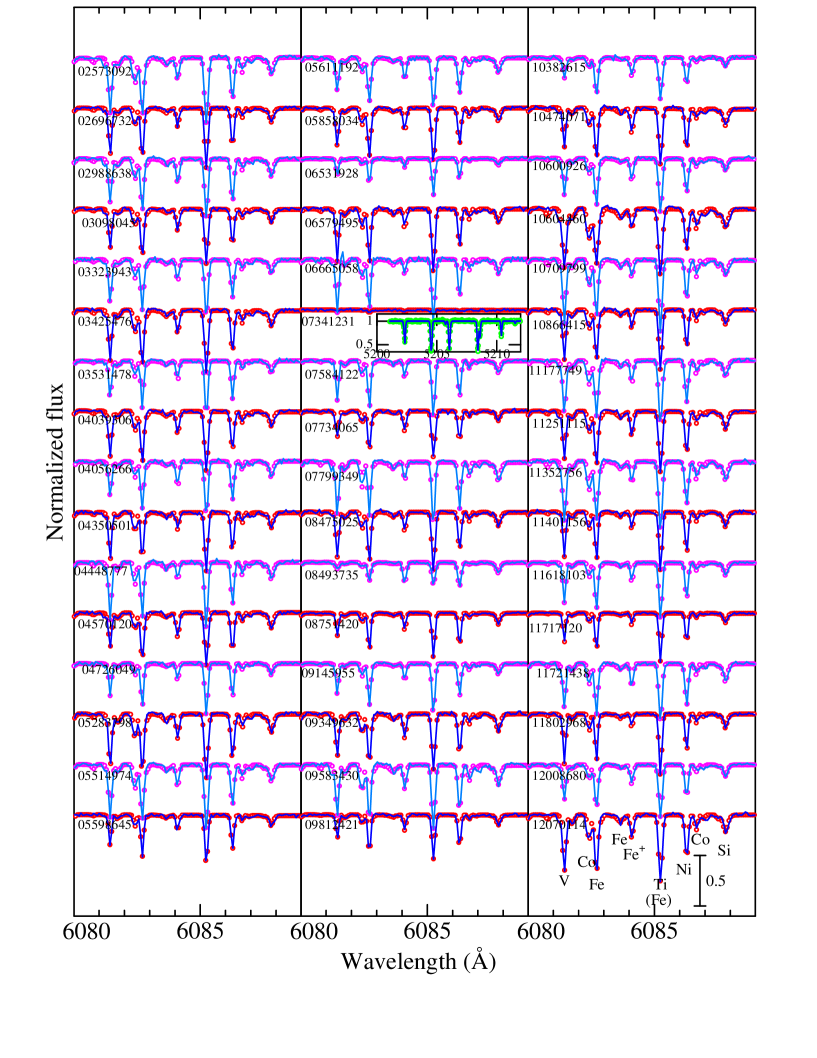
Figure 3: Synthetic spectrum fitting in the 6080–6089 $\rm\AA$ region accomplished by varying the abundances of Si, Ti, V, Fe, Co, and Ni, along with the macrobroadening parameter and the wavelength shift (radial velocity). The best-fit theoretical spectra are shown by solid lines, while the observed data are plotted by symbols, where the wavelength scale of the stellar spectrum has been adjusted to the laboratory frame. Each spectrum is vertically shifted by 0.5 relative to the adjacent one. Note that spectrum fitting at the 5200–5212 $\rm\AA$ region was specially applied to KIC 07341231 (as shown in the inset), since the lines in the 6080–6089 $\rm\AA$ region are too weak. The spectra are arranged in the same order as in Fig. 1.

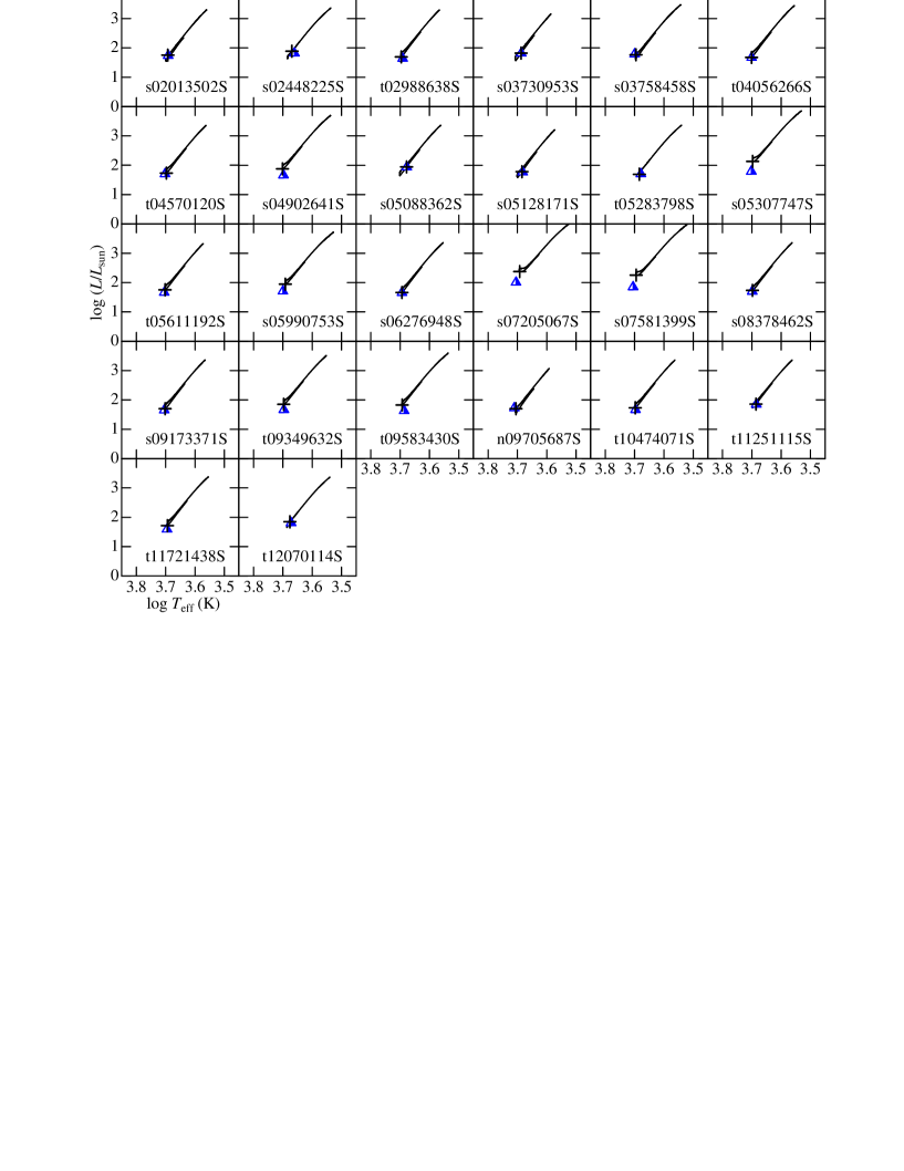
Figure 7: Comparison of the observed ($\log T_{\rm eff}$, $\log L/{\rm L}_{\odot}$) with the assigned theoretical evolutionary track for 26 RC2-class stars. In each panel, the actual stellar location is indicated by a blue triangle. Otherwise, the same as in Fig. 5.

Appendix A Metallicity-dependence in the scaling relation?

One of the aims in Paper I was to examine the consistency between the spectroscopic $\log g_{\rm spec}$ and the seismic $\log g_{\rm seis}$. Now that the sample size has been almost doubled, it would be worthwhile to recheck this matter again. The correlation between $\log g_{\rm spec}$ and $\log g_{\rm seis}$ is shown in Fig. A1a, while the $\Delta\log g$(spec$-$seis) difference is plotted against $T_{\rm eff}$, $\log g$, and [Fe/H] in Fig. A1b, A1c, and A1d, respectively. We can confirm from these figures the same characteristics as concluded in Paper I; i.e., (i) $\log g_{\rm spec}$ and $\log g_{\rm seis}$ satisfactorily agree with each other (with the standard deviation of $\sigma\sim 0.1$ dex) and (ii) $\Delta\log g$(spec$-$seis) difference does not show any systematic dependence upon $T_{\rm eff}$ and $\log g$.

We also point out that this conclusion for $\Delta\log g$(spec$-$seis) holds regardless of the evolutionary status (RG/RC1/RC2). Although Pinsonneault et al. (2014) recently carried out an extensive analysis on the stellar parameters of a large number of red giants in the Kepler field and reported a systematic disagreement in $\Delta\log g$(spec$-$seis) between RG and RC1/RC2 (i.e., negative for the former while positive for the latter; cf. Fig. 3 of their paper), such a trend can not be observed in our results.

Interestingly, however, we newly noticed a slight metallicity-dependent trend in $\Delta\log g$(spec$-$seis), in the sense that $\Delta\log g$(spec$-$seis) tends to increase with a decrease in [Fe/H], as shown in Fig. A1d. It is hard to consider that such a [Fe/H]-dependence exists in spectroscopic gravities for the following reasons:
— The difference in the metallicity for each star, which affects the opacity, is properly taken into account in model atmospheres in our analysis.
— It is unlikely that the non-LTE effect (non-LTE overionization of Fe i) is responsible, because it should lead to an underestimation of $\log g_{\rm spec}$ which becomes more conspicuous as the metallicity is lowered. That is, if this effect appreciably exists, $\Delta\log g$(spec$-$seis) would decrease with a decrease in [Fe/H], which is just the opposite to the trend seen in Fig. A1d.

We, therefore, suspect that this effect may be attributed to $\log g_{\rm seis}$. Here, the scaling relation for $\nu_{\rm max}(\propto gT_{\rm eff}^{-1/2})$ is relevant (while $\Delta\nu$ is irrelevant) in deriving $g_{\rm seis}$ (cf. Eq.(3) in Paper I). However, this relation for $\nu_{\rm max}$, which was first proposed by Kjeldsen & Bedding (1995) in analogy with acoustic cut-off frequency, is not so much physically justified as rather an empirically useful relation (e.g., Bedding & Kjeldsen 2003). Actually, Belkacem et al. (2013) discussed based on their model calculation that this relation seems sufficiently good for dwarfs but some discrepancies (by up to $\sim 15$%) may arise for giants. Accordingly, given that there is still room for further improvement for the expression of $\nu_{\rm max}$, it may possibly depend upon the metallicity in some way.

Appendix B Mass-determination problem revisited

In Paper I was studied how the stellar mass of a red giant star derived from evolutionary tracks ($M_{\rm trk}$) by following Takeda et al.’s (2008) procedure is compared with the seismic mass ($M_{\rm seis}$). They found that $M_{\rm trk}$ tends to be considerably overestimated (typically by $\sim 50$% on the average) for RC-stars (cf. Fig. 12a therein), which means that the mass values of many red clump giants in Takeda et al.’s (2008) sample must also be systematically too large.

Unfortunately, in Paper I, the direct $M_{\rm seis}$ vs. $M_{\rm trk}$ was possible only for 9 Kepler giants (1 for RG, 6 for RC1, and 2 for RC2), because $L$ was determined from the apparent magnitude in the same manner as in Takeda et al. (2008) while the parallax data were available only for a limited number of stars. Since we have established this time the $L$ values for all 106 stars by combining $T_{\rm eff,spec}$ and $R_{\rm seis}$, we decided to revisit this problem based on this large sample.

In this test, we derived $M_{\rm trk}$ in three different ways:
— (a) Exactly the same procedure as adopted by Takeda et al. (2008) was followed; i.e., combined RG+RC tracks of Lejeune & Schaerer’s (2001) grid for various mass values were used as if neither the mass nor the evolutionary status of each star were known (see Sect. 4.2 in Paper I for more details).
— (b) Combined RG+RC tracks of the PARSEC grid (for various mass values but with the assigned $z_{\rm grid}$ closest to actual stellar metallicity) were used as if neither the mass nor the evolutionary status of each star were known. That is, $M_{\rm trk}$ was determined by searching for the minimum $d^{2}$ on the $(M,t)$ plane after trying all possible RG+RC tracks.
— (c) Either RG or RC tracks of the PARSEC grid (for various mass values but with the assigned $z_{\rm grid}$ closest to actual stellar metallicity) were appropriately used depending on the known evolutionary status of each star. That is, $M_{\rm trk}$ was determined by searching for the minimum $d^{2}$ on the $(M,t)$ plane after trying all possible RG tracks (for RG class) or RC tracks (for RC1 or RC2 classes).

The resulting $M_{\rm trk}$ vs. $M_{\rm seis}$ plots corresponding to these three cases are depicted in Fig. B1a, Fig. B1b, and Fig. B1c, respectively. We can see that Fig. B1a is quite consistent with Fig. 12a in Paper I, indicating a considerable overestimation of $M_{\rm trk}$ for RC1 stars (red clump stars of lower mass), while the discrepancy is not so large for RC2 stars (red clump stars of higher mass) where $M_{\rm trk}$ tends to be even somewhat smaller than $M_{\rm seis}$ at the high-mass end ($M\ga 3{\rm M}_{\odot}$). We suspect that the reason why the considerably large overestimation of $M_{\rm trk}$ derived by Takeda et al.’s (2008) procedure is seen only in RC1 stars (but not in RC2 stars) is mainly due to the lack of “He flash” RC tracks for lower mass stars ($M<2$ M_⊙) in Lejeune & Schaere’s (2001) data (cf. Fig. A1d in Paper I), rather than the ignorance of the evolutionary status. Actually, we can recognize from the comparison of Fig. B1b and Fig. B1c that the degree of consistency between $M_{\rm trk}$ and $M_{\rm seis}$ is nearly the same for both case (b) [combined RG+RC tracks were indifferently used] and case (c) [either RG or RC tracks were appropriately assigned]. This may suggest that the knowledge of the evolutionary status (RG or RC) in advance is not necessarily essential for deriving $M_{\rm trk}$ (in the sense that such information does not significantly improve the situation), for which sufficiently fine and wide coverage of the ($z$, $M$) grid in the adopted theoretical tracks (as well as defining the stellar position on the HR diagram as precisely as possible) would be more important.

References

- [] Asplund M., Grevesse N., Sauval A. J., Scott P., 2009, ARA&A, 47, 481
- [] Bedding T. R., et al., 2011, Nature, 471, 608
- [] Bedding T. R., Kjeldsen H., 2003, PASA, 20, 203
- [] Belkacem K., Samadi R., Mosser B., Goupil M.-J., Ludwig H.-G., 2013, in Progress in Physics of the Sun and Stars: A New Era in Helio- and Asteroseismology, ASP Conf. Ser, Vol. 479, eds. H. Shibahashi & A. E. Lynas-Gray, p. 61 (San Francisco: Astronomical Society of the Pacific)
- [] Bergemann M., et al., 2014, A&A, 565, A89
- [] Bressan A., Marigo P., Girardi L., Salasnich B., Dal Cero C., Rubele S., Nanni A., 2012, MNRAS, 427, 127
- [] Bressan A., Marigo P., Girardi L., Nanni A., Rubele S., 2013, EPJ Web of Conferences, 43, 3001 (DOI: http://dx.doi.org/10.1051/epjconf/20134303001)
- [] Brown T. M., Latham D. W., Everett M. E., Esquerdo G. A., 2011, AJ, 142, 112
- [] Casagrande L., et al., 2014, ApJ, 781, 110
- [] Casagrande L., et al., 2016, MNRAS, 455, 987
- [] Kjeldsen H., Bedding T. R., 1995, A&A, 293, 87
- [] Lejeune T., Schaerer D., 2001, A&A, 366, 538
- [] Mosser B. et al., 2012, A&A, 540, A143
- [] Pinsonneault M. H., et al., 2014, ApJS, 215, 19
- [] Takeda Y., 2007, PASJ, 59, 335
- [] Takeda Y., Honda S., Aoki W., Takada-Hidai M., Zhao G., Chen Y.-Q., Shi J.-R., 2006, PASJ, 58, 389
- [] Takeda Y., Ohkubo M., Sato B., Kambe E., Sadakane K., 2005, PASJ, 57, 27 (Erratum 57, 415)
- [] Takeda Y., Sato B., Murata D., 2008, PASJ, 60, 781
- [] Takeda Y., Tajitsu A., 2015, MNRAS, 450, 397 (Paper I)
- [] Thygesen A. O. et al., 2012, A&A, 543, A160