Ultracold molecular Rydberg physics in a high density environment

Abstract

Sufficiently high densities in Bose-Einstein condensates provide favorable conditions for the production of ultralong-range polyatomic molecules consisting of one Rydberg atom and a number of neutral ground state atoms. The chemical binding properties and electronic wave functions of these exotic molecules are investigated analytically via hybridized diatomic states. The effects of the molecular geometry on the system’s properties are studied through comparisons of the adiabatic potential curves and electronic structures for both symmetric and randomly configured molecular geometries. General properties of these molecules with increasing numbers of constituent atoms and in different geometries are presented. These polyatomic states have spectral signatures that lead to non-Lorentzian line-profiles.

• March 3, 2024
  *corresponding author

1 Introduction

Exotic dimers consisting of a Rydberg atom bound to a neutral ground state atom possess many fascinating properties, such as their oscillatory potential energy curves, extremely large bond lengths, complex nodal wave functions and, in the polar “trilobite” case, huge permanent electric dipole moments  [1, 2, 3, 4, 5]. In recent years, non-polar long-range Rydberg molecules consisting primarily of $ns$ [6], $np$ [7] and $nd$ [8, 9, 10] states have been observed in Rb condensates, and a polar trilobite molecule exhibiting a kilo-debye permanent electric dipole moment has been photoassociated in Cs  [11]. Rydberg molecules have been formed in an optical lattice, providing a non-destructive probe of the Mott transition [12]. Recently, molecular formation in non-alkali atomic species have been explored [13, 14].

Current experiments can excite very high Rydberg states in dense condensates so the Rydberg electron’s orbit encloses more than one ground state atom, increasing the probability of forming polyatomic molecules [15, 16]. At higher densities and excitation energies even the coupling between the Rydberg electron and the entire condensate [17, 18] can be studied; in this regime the spectrum no longer exhibits few-body molecular lines but rather demonstrates a density shift [19] possibly requiring a mix of few and many-body approaches [20, 21]. Theoretical efforts in this area have predicted the formation of Borromean trimers [22] and investigated the breathing modes of coplanar molecules [23]. These investigations have only included $s$-wave scattering, which neglects essential physics, particularly relevant at high density [15, 20]. Very recently a Rydberg trimer including $p$-wave scattering and electric field effects has been investigated [24]

This present work develops an accurate theoretical framework incorporating $p$-wave scattering that robustly generalizes to any number of constituent atoms in an arbitrary molecular shape. General formulas are provided for the electronic wave functions and Born-Oppenheimer adiabatic potential energy curves (APECs) in terms of linear combinations of the diatomic “trilobite” [1] and “butterfly” [2] wave functions; construction of these hybridized orbitals is aided by adapting them to the molecular symmetry point group using the projection operator method [25, 26]. A key result of this study is that the level spacings, degeneracies, and adiabatic/diabatic level crossing properties of these systems are determined by hybridized orbitals reflecting the molecular geometry. This represents a necessary step towards an accurate understanding of experimental spectra in increasingly dense environments.

This work is organized as follows: section 2.1 describes the polyatomic Hamiltonian and outlines the full solution via numerical diagonalization. In section 2.2, the properties of the diatomic molecular states are studied in detail, so that in section 2.3 the polyatomic Schrödinger equation can be solved by construction of linear combinations of these diatomic orbitals. In section 2.4, these results are specialized to highly symmetric molecules. Section 3 presents results for a variety of molecular geometries. The reliability and accuracy of the analytic approximations is demonstrated and the effects of symmetry on the molecular spectra and properties are examined in detail. Section 3.4 describes some of the properties of polyatomic molecules formed from low angular momentum Rydberg states, which are relevant to current experimental efforts. Finally, in section 4, the general effects of increasing the number of atoms are studied for the trilobite states, and section 5 concludes with a discussion of experimental proposals for controlled formation of highly symmetric polyatomic molecules.

2 Theoretical approach

2.1 Pseudopotential and Basis Diagonalization

The polyatomic system consists of $N$ ground state atoms, located at $\vec{R}_{i}=(R_{i},\theta_{i},\varphi_{i})$, surrounding a central Rydberg atom. For tractability, the molecular breathing modes, where the ground state atoms share a common distance $R_{i}=R$ to the Rydberg core, are the primary focus of this study. The $n=30$ states of rubidium are studied to connect with previous work [1, 23], but the general framework applies to any Rydberg state of an alkali with a negative scattering length. Within the Born-Oppenheimer approximation, the nuclei of all atoms are assumed to be stationary with respect to the electronic motion. The Rydberg electron interacts with each neutral atom through the $s$-wave Fermi pseudopotential along with the p-wave scattering term due to Omont [27, 28]. Since the scale of the Rydberg orbit extends over a far greater range than any interatomic potentials, the Hamiltonian only includes the unperturbed atomic Hamiltonian, $H_{0}$, and $N$ pseudopotentials:

$$\hat{H}_{N}({\vec{r}})=\hat{H}_{0}+\sum_{i=1}^{N}\hat{V}(\vec{r},\vec{R}_{i})$$ (1)

$$\hat{V}(\vec{r},\vec{R}_{i})=2\pi\delta({\vec{r}}-{\vec{R}_{i}})\Big{(}a_{s}[k(R)]+3a_{p}^{3}[k(R)]{\reflectbox{$\vec{\reflectbox{$\nabla$}}$}_{r}}\cdot{\vec{\nabla}_{r}}\Big{)}.$$

Atomic units are used throughout. The triplet $s$-wave scattering length $a_{s}$ and $p$-wave scattering volume $a_{p}^{3}$ depend on $R$ through the semiclassical relationship $k^{2}/2=E_{n}-1/R$; the singlet scattering length is an order of magnitude smaller and is ignored. These parameters depend on the energy-dependent triplet scattering phase shifts $\delta_{0}^{T}$ and $\delta_{1}^{T}$ [29] through the relationships

$$\begin{split}&a_{s}[k(R_{i})]=-\frac{\tan\left(\delta_{0}^{T}[k(R)]\right)}{[k(R)]},\\ &a_{p}^{3}[k(R_{i})]=-\frac{\tan\left(\delta_{1}^{T}[k(R)]\right)}{[k(R)]^{3}}.\end{split}$$ (2)

The APECs are obtained by diagonalizing equation (1) in a basis of hydrogenic eigenstates $\phi_{nlm}(\vec{r})=R_{nl}(r)Y_{lm}(\theta,\varphi)$ of the unperturbed Hamiltonian $H_{0}$,

$$\left(\hat{H}_{0}+\frac{1}{2(n-\mu_{l})^{2}}\right)|{\phi_{nlm}}\rangle=0,$$ (3)

where $\mu_{l}$ is the quantum defect for a given angular momentum $l$ relative to the Rydberg core. Two significant difficulties complicate this approach. Rubidium, along with several other alkali species, possesses a $p$-wave shape resonance that creates an unphysical divergence in the APECs. This is remedied by enlarging the basis size to include additional hydrogenic manifolds adjacent to the manifold of interest, giving sensible results due to level repulsion between states of opposite symmetry [2]. This introduces a more serious problem: the delta function potential formally diverges, so the APECs do not converge with the addition of more adjacent manifolds [30], and in fact begin to yield worse results with increasing basis size in comparison with sophisticated Green function techniques that exactly solve the diatomic Hamiltonian. In the following numerical results the basis consists of the $n$, $n\pm 1$ hydrogenic manifolds, which we have found agrees well with the Green function method in the diatomic case.

2.2 $N=1$: Diatomic molecular features

2.2.1 States of low angular momentum:

Two distinct classes of APECs, characterized by the unperturbed Rydberg electron’s angular momentum, emerge from the diagonalization. The non-zero quantum defects of low-$l$ states separate them energetically from the nearly degenerate high-$l$ ($l\geq 3$ for Rb) manifold. The APECs for low-$l$ states are tens to hundreds of MHz in depth and support only a few weakly bound molecular states. The first order APEC for the $|{nlm}\rangle$ state including only the $s$-wave interaction is proportional to the Rydberg electron’s wave function and, due to the symmetry provided by the internuclear axis, is only non-zero for $m_{l}=0$:

$$\tilde{E}_{l\leq 2,0}(R)=2\pi a_{s}[k(R)]\left(\frac{u_{nl}(R)}{R}\right)^{2}\left|Y_{l0}(0,0)\right|^{2}.$$ (4)

2.2.2 “Trilobite” and “butterfly” states of mixed high angular momentum:

In contrast, four strongly perturbed high-$l$ eigenstates form out of the degenerate high-$l$ states: the “trilobite” state, dominated by s-wave scattering, and three “butterfly” states - “$R$-butterfly,” “$\theta$-butterfly,” and “$\varphi$-butterfly - corresponding to the three directional derivatives in the p-wave interaction. Their APECs are nearly an order of magnitude deeper than the low-$l$ states. As will be seen in the following sections, coherent sums of these diatomic states fully describe the polyatomic states, and so they are studied in detail to clearly elucidate their properties.

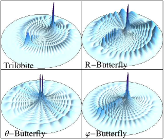
Figure 1: Planar cuts of the probability amplitudes $\sqrt{r^{2}\Psi(x,y,z)^{2}}$ of the fundamental diatomic eigenstates. The $\theta$-butterfly lies in the $yz$ plane; the three others in the $xy$ plane. $R=840$ a.u for the trilobite and $345$ a.u. for the three butterfly states. The Rydberg core is at the center of each figure and the neutral atom is underneath the most prominent spikes.

Due to the particular properties of the $s$- and $p$-wave delta-function potentials in equation (1), the diatomic eigenstates, eigenenergies, and overlap matrix elements for these high-$l$ states can be written [22] as elements of a ($4\times 4)\otimes(N\times N$) “trilobite overlap matrix”, $\mathbf{\Upsilon_{pq}^{\boldsymbol{\alpha}\boldsymbol{\beta}}}$, where $\left(\mathbf{\Upsilon_{pq}^{\boldsymbol{\alpha}\boldsymbol{\beta}}}\right)^{*}=\mathbf{\Upsilon_{qp}^{\boldsymbol{\beta}\boldsymbol{\alpha}}}$. The lower indices $p$ and $q$ label the position vectors $\vec{R}_{p}$ and $\vec{R}_{q}$ of two neutral atoms; a lower index $r$ indicates $\vec{R}_{r}=\vec{r}$. Upper indices $\alpha$ and $\beta$ label the eigenstates: the normalized $\xi$th eigenstate associated with an internuclear axis $\vec{R}$ is given by $\mathbf{\Upsilon_{Rr}^{\boldsymbol{\xi}1}}/\sqrt{\mathbf{\Upsilon_{RR}^{\boldsymbol{\xi}\boldsymbol{\xi}}}}$. After defining $a_{\xi=1}=a_{s}$ and $a_{\xi\geq 2}=3a_{p}^{3}$ the trilobite ($\xi=1$) and three ($R$, $\theta$, $\varphi$)-butterfly APECs $(\xi=2,3,4)$ have the concise form:

$$E_{l>3}^{\xi}(R) =2\pi a_{\xi}[k(R)]\mathbf{\Upsilon_{RR}^{\boldsymbol{\xi}\boldsymbol{\xi}}}.$$ (5)

The trilobite overlap matrix is defined as

$$\mathbf{\Upsilon_{pq}^{\boldsymbol{\alpha}\boldsymbol{\beta}}}=\sum_{l=3}^{n-1}\sum_{m=-l}^{m=l}\left[\Phi^{\alpha}_{nlm}(\vec{R}_{p})\right]^{*}\Phi^{\beta}_{nlm}(\vec{R}_{q}),$$ (6)

where the summation extends over energetically degenerate states, starting at $l=3$ for Rb. $\Phi^{\alpha}_{nlm}$ labels the wave function and components of the gradient in spherical coordinates:

$$\Phi^{\alpha}_{nlm}(\vec{r})=\begin{cases}\phi_{nlm}(\vec{r})&\alpha=1\\ \frac{\partial{\phi_{nlm}(\vec{r})}}{\partial{r}}&\alpha=2\\ \frac{1}{R}\frac{\partial{\phi_{nlm}(\vec{r})}}{\partial{\theta}}&\alpha=3\\ \frac{1}{R\sin\theta}\frac{\partial{\phi_{nlm}(\vec{r})}}{\partial{\varphi}}&\alpha=4.\end{cases}$$ (7)

If the low-$l$ states are included in equation (6), the trilobite eigenstate can be summed analytically using the Green function for the Coulomb problem [31]

$$\mathbf{\Upsilon_{Rr}^{11}}=\frac{u_{n0}^{\prime}(t_{-})u_{n0}(t_{+})-u_{n0}(t_{-})u_{n0}^{\prime}(t_{+})}{4\pi\Delta t},$$ (8)

$$\Delta t=t_{+}-t_{-},$$

$$t_{\pm}=\frac{1}{2}\left(R+r\pm\sqrt{R^{2}+r^{2}-2Rr\cos\gamma}\right),$$

where $\gamma$ is the angle between $\vec{R}$ and $\vec{r}$. This expression is a good approximation for the summation in equation (6) for energies between the high-$l$ manifold and the low-$l$ states with nonzero quantum defects. The three butterfly eigenstates can be found by differentiating equation (8) with respect to $R$, $\theta_{R}$, and $\varphi_{R}$:

$$\mathbf{\Upsilon_{Rr}^{21}}=\frac{(r\cos\gamma-R)\mathcal{F}(t_{+},t_{-})}{8\pi\Delta t^{3}}$$ (9)

$$\,\,\,\,\,\,\,\,\,\,\,\,+\frac{u_{n0}(t_{+})u_{n0}^{\prime\prime}(t_{-})-u_{n0}(t_{-})u_{n0}^{\prime\prime}(t_{+})}{8\pi\Delta t}$$

$$\mathbf{\Upsilon_{Rr}^{31}}=\cos\theta_{R}\cos\varphi_{R}\Upsilon_{x}+\cos\theta_{R}\sin\varphi_{R}\Upsilon_{y}-\sin\theta_{R}\Upsilon_{z}$$ (10)

$$\mathbf{\Upsilon_{Rr}^{41}}=-\sin\varphi_{R}\Upsilon_{x}+\cos\varphi_{R}\Upsilon_{y},$$ (11)

where

$$\Upsilon_{x,y,z}=\frac{\mathcal{F}(t_{+},t_{-})}{8\pi(\Delta t)^{3}}(\sin\theta_{r}\cos\varphi_{r},\sin\theta_{r}\sin\varphi_{r},\cos\theta_{r}),$$

$$\mathcal{F}(t_{+},t_{-})=-2(\Delta t)u_{n0}^{\prime}(t_{+})u_{n0}^{\prime}(t_{-})$$

$$\,\,\,\,\,\,\,\,-u_{n0}(t_{-})[2u_{n0}^{\prime}(t_{+})-(\Delta t)u_{n0}^{\prime\prime}(t_{+})]$$

$$\,\,\,\,\,\,\,\,+u_{n0}(t_{+})[2u_{n0}^{\prime}(t_{-})+(\Delta t)u_{n0}^{\prime\prime}(t_{-})].$$

The $\theta,\varphi$ butterfly orbitals can be identified as vectors of magnitude $\frac{\mathcal{F}(t_{+},t_{-})}{8\pi(\Delta t)^{3}}$ parallel to the $\theta,\varphi$ unit vectors; the trilobite and $R$-butterfly orbitals are fully symmetric about the internuclear axis. The diagonal elements $\mathbf{\Upsilon_{pp}^{\xi\xi}}$ are obtained by evaluating equations (8 - 11) in the limit $\vec{R}_{p}\to\vec{R}_{q}$:

$$\mathbf{\Upsilon_{RR}^{11}}=\frac{(2n^{2}-R)\left(u_{n0}(R)/n\right)^{2}+Ru_{n0}^{\prime}(R)^{2}}{4\pi R}$$ (12)

$$\mathbf{\Upsilon_{RR}^{22}}=\mathbf{\Upsilon_{RR}^{33}}-\frac{u_{n0}(R)}{12\pi R^{3}}\left[3Ru^{\prime}_{n0}(R)+2u_{n0}(R)\right]$$ (13)

$$\mathbf{\Upsilon_{RR}^{33}}=\mathbf{\Upsilon_{RR}^{44}}$$ (14)

$$\,\,\,\,\,\,\,\,\,\,\,\,\,\,=\frac{4\pi R(2n^{2}-R)\mathbf{\Upsilon_{RR}^{11}}-n^{2}u_{n0}^{\prime}(R)u_{n0}(R)}{12\pi n^{2}R^{2}}.$$

The diatomic angular butterfly APECs, $\mathbf{\Upsilon_{RR}^{33}}$ and $\mathbf{\Upsilon_{RR}^{44}}$, are degenerate ${}^{3}\Pi$ molecular states and, in contrast to the ${}^{3}\Sigma$ trilobite or $R$-butterfly APECs, do not oscillate as a function of $R$. This is due to destructive interference between terms in the numerator of equation (14).

The full Hamiltonian is solved by assuming a linear combination of the eigenstates in equation (6) as a solution [32]. Two additional properties of the overlap matrix are important. $\mathbf{\Upsilon_{pq}^{\boldsymbol{\alpha}\boldsymbol{\beta}}}$ is the overlap between different diatomic orbitals $\alpha$ and $\beta$ associated with different ground state atoms located at $\vec{R}_{p}$ and $\vec{R}_{q}$, respectively, and the matrix element of the $\xi$th interaction term of the Hamiltonian between an orbital $\alpha$ located at $\vec{R}_{p}$ and an orbital $\beta$ located at $\vec{R}_{q}$ is $\mathbf{\Upsilon_{ip}^{\boldsymbol{\xi}\boldsymbol{\alpha}}}\mathbf{\Upsilon_{qi}^{\boldsymbol{\beta}\boldsymbol{\xi}}}$. A generalized eigenvalue equation for $E(R)$ is then obtained:

$$\sum_{\beta=1}^{4}\left(\sum_{\xi=1}^{4}a_{\xi}(k)\mathbf{\Upsilon_{RR}^{\boldsymbol{\xi}\boldsymbol{\alpha}}}\mathbf{\Upsilon_{RR}^{\boldsymbol{\beta}\boldsymbol{\xi}}}-\frac{E}{2\pi}\mathbf{\Upsilon_{RR}^{\boldsymbol{\alpha}\boldsymbol{\beta}}}\right)\Omega^{\beta}_{R}=0.$$ (15)

Throughout the rest of this paper the explicit dependence of $k$, $E$, and the eigenvector $\vec{\Omega}$ on the internuclear distance $R$ is assumed for brevity.

2.3 $N=$ many: Generalization to polyatomic molecular states

The diatomic results described above readily generalize to the $N>1$ case. For the low-$l$ APECs, all $m_{l}$ values are allowed; therefore $N_{d}=2l+1$ degenerate $m_{l}$ states mix together. This causes $N_{p}=\max(4N,N_{d})$ APECs to split away from the unperturbed electronic states. For the $s$-wave interaction alone the APECs are the eigenvalues $E(R)$ given by the matrix equation

$$a_{s}(k)\left(\frac{u_{nl}(R)}{R}\right)^{2}\sum_{m=-l}^{l}\sum_{i=1}^{N}Y_{lm^{\prime}}^{*}(\theta_{i},\varphi_{i})Y_{lm}(\theta_{i},\varphi_{i})\Omega_{m}^{1}$$

$$=\frac{E}{2\pi}\Omega_{m^{\prime}}^{1}.$$ (16)

The trilobite overlap matrix formalism allows for rapid generalization to the polyatomic system, since the trial solution used to obtain equation (15) is expanded to include linear combinations of trilobite and butterfly eigenstates for each diatomic Rydberg-neutral pair:

$$\Psi(\vec{r})=\sum_{p=1}^{N}\sum_{\alpha=1}^{4}\Omega_{p}^{\alpha}\mathbf{\Upsilon_{pr}^{\boldsymbol{\alpha}1}}.$$ (17)

This formulation provides key physical insight and also greatly reduces the calculational effort to the diagonalization of at most a $4N\times 4N$ matrix, rather than the full $n^{2}\times n^{2}$ basis size needed to diagonalize equation (1). The trilobite APECs, only including the $s$-wave interaction, are the eigenvalues $E(R)$ satisfying

$$\sum_{q=1}^{N}\left(a_{s}(k)\mathbf{\Upsilon_{pq}^{11}}-\frac{E}{2\pi}\mathbf{\boldsymbol{\delta}_{pq}}\right)\Omega_{q}^{1}=0.$$ (18)

The p-wave interaction is included analogously to the diatomic case, yielding a generalized eigenvalue problem with a $4N\times 4N$ matrix:

$$\sum_{\beta=1}^{4}\sum_{p,q=1}^{N}\Bigg{(}\sum_{\xi=1}^{4} \sum_{i=1}^{N}a_{\xi}(k)\mathbf{\Upsilon_{ip}^{\boldsymbol{\xi}\boldsymbol{\alpha}}}\mathbf{\Upsilon_{qi}^{\boldsymbol{\beta}\boldsymbol{\xi}}}-\frac{E}{2\pi}\mathbf{\Upsilon_{pq}^{\boldsymbol{\alpha}\boldsymbol{\beta}}}\Bigg{)}\Omega_{q}^{\beta}=0.$$ (19)

Equations (2.3-19) accurately reproduce the full diagonalization results for arbitrary molecular configurations and numbers of atoms, particularly for the trilobite states. Due to the challenges with basis set diagonalization described in section (2.1), spectroscopic accuracy for the low-$l$ states can only be achieved through a careful convergence study [20] or with the Green function method. As a result, equations (4) and (2.3) should only be used for qualitative study. For the $n=30$ system studied here, the $l=0$ states are about 20% deeper than these first-order results predict. In contrast, the high-$l$ APECs are quite accurate. Since only one manifold is included, these formulas break down at internuclear distances smaller than the location of the $p$-wave shape resonance, and also do not describe couplings with low$-l$ states at large detunings. For investigations in regimes where these inaccuracies are irrelevant, equation (19) is a valuable computational advance, particularly for experiments probing high Rydberg states up to $n\sim 110$ [18, 20] due to the reduced basis size.

The off-diagonal elements of $\mathbf{\Upsilon_{pq}^{\boldsymbol{\alpha}\boldsymbol{\beta}}}$, corresponding to the overlap between orbitals associated with different Rydberg-neutral pairs, determine the size of the differences between the polyatomic states and the $N=1$ state. In the absence of these overlaps equation (19) is diagonal in the lower indices and all $N$ polyatomic APECs converge to the diatomic APEC. At large $R$ the overlap between orbitals vanishes, and the APECs are seen to converge to the diatomic limit. Co-planar molecules typically exhibit larger splittings than three-dimensional molecules for this same reason. Additionally, as $N$ grows the system will deviate more strongly from the $N=1$ case; this causes the global minimum of the APECs to deepen with $N$. The angular dependence of the trilobite wave functions contributes considerably to the energy landscape of the system at hand, especially when two ground state atoms are close in proximity and therefore have a large overlap. More stable Rydberg molecules can thus be engineered by exploiting these features.

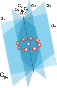
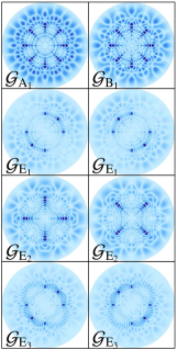
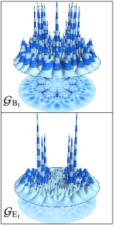
Figure 2: (a) The symmetry operations for $C_{8v}$ symmetry. The $\sigma_{d}$ reflection planes bisect the lines between ground state atoms and are not shown for clarity. (b) “Hoodoo” symmetry adapted orbitals for trilobite states of an octagonal molecule with internuclear distance $R=840$ a.u. The probability amplitude $\sqrt{r^{2}|\psi(x,y,0)|^{2}}$ is plotted in the $xy$ plane. (c) The electron probability corresponding to the one-dimensional irrep $B_{1}$ (top) and one of the doubly-degenerate $E_{1}$ irreps (bottom) are plotted.

2.4 Symmetry-adapted orbitals

2.4.1 Molecular symmetry point groups.

To fully understand the structure of these APECs, in particular the appearance of degeneracies and level crossings in highly symmetric molecular geometries and the effects of the molecular symmetry on the coupling between trilobite and butterfly states, it is mandatory to characterize the symmetry group of the molecule. The molecular symmetry group is a subgroup of the complete nuclear permutation inversion group of the molecule [25, 26], which commutes with the molecular Hamiltonian in free space. Therefore, the eigenstates of such a Hamiltonian can be classified in terms of the irreducible representations (irreps) of the given molecular symmetry group, called symmetry-adapted orbitals (SAOs). Given a molecular symmetry group, it is possible to calculate the SAOs associated with each irrep of the group using the projection operator method, where the projection operator is [25]

$$\hat{\mathcal{P}}^{j}=\frac{l_{j}}{h}\sum_{i=1}^{h}\chi_{ji}\mathcal{R}_{i}.$$ (20)

The index $j$ labels the different irreps and $i$ denotes the group elements. These are the familiar symmetry operations: rotations, reflections, and inversions. $\mathcal{R}_{i}$ represents the operator associated with the $i$th symmetry operation; $l_{j}$ and $\chi_{ji}$ represent the dimension and character for the $i$th operation, respectively. Finally, $h$ stands for the order of the group. The trace of the projection operator, $\tr\hat{\mathcal{P}}^{j}=l_{j}$, determines the decomposition of the point group into irreps. All irreps with $l_{j}\neq 0$ are contained. SAOs associated with different irreps have different parity under the molecular symmetry group, and hence will exhibit real crossings. $l_{j}$ determines the degeneracy of each irrep.

The projection operator also gives the coefficients $\mathcal{A}_{p}^{(\alpha,j)}$ for the SAO $\mathcal{G}^{(\alpha,j)}(\vec{r})$ corresponding to the $\alpha$th orbital and $j$th irrep:

$$\mathcal{G}^{(\alpha,j)}(\vec{r})=\sum_{p=1}^{N}\mathbf{\Upsilon_{pr}^{\boldsymbol{\alpha}\boldsymbol{1}}}\mathcal{A}_{p}^{(\alpha,j)}.$$ (21)

The prescription for calculating the projection operator depends on the orbital in question. The ${}^{3}\Sigma$ trilobite and $R$-butterfly states can be symmetry-adapted independently since they are non-degenerate. Since these orbitals are symmetric about the Rydberg-neutral internuclear axis the symmetry operations leave the orbitals unchanged except for an overall transformation of the atomic positions within the molecule, i.e. a permutation of the basis of Rydberg-neutral pairs at different positions $\psi_{p}$: $\vec{\Psi}=(\psi_{A},\psi_{B},...,\psi_{N})^{T}$. The $N\times N$ matrix representations of the symmetry operations can then be identified with a modicum of effort and the sum in (20) performed. The orthogonalized rows of $\hat{\mathcal{P}}^{j}$ provide the coefficients.

Since the $\theta$ and $\varphi$ butterfly ${}^{3}\Pi$ states are degenerate, these orbitals can be mixed by symmetry operations, so these orbitals must be symmetry-adapted together. The basis size is doubled to allow mixing: $\vec{\Psi}=(\psi^{\theta}_{A},\psi^{\theta}_{B},...,\psi^{\theta}_{N},\psi^{\varphi}_{A},\psi^{\varphi}_{B},...,\psi^{\varphi}_{N})^{T}$. The effect of a symmetry operation on the entire molecule transforms orbitals located at one Rydberg-neutral pair to another as in the trilobite/$R$-butterfly case: $\psi^{\theta}_{i}\to\psi^{\theta}_{i^{\prime}}$ and $\psi^{\varphi}_{i}\to\psi^{\varphi}_{i^{\prime}}$. However, the symmetry operation now modifies the orbitals themselves. The angular butterfly orbitals are vectors in Cartesian coordinates (see equations (10-11)) and the symmetry operators in the $xyz$ coordinate basis affect them. This transforms $\psi^{\theta}_{i}\to\alpha\psi^{\theta}_{i^{\prime}}+\beta\psi^{\varphi}_{i^{\prime}}$ and $\psi^{\varphi}_{i}\to\gamma\psi^{\theta}_{i^{\prime}}+\delta\psi^{\varphi}_{i^{\prime}}$; the coefficients $\alpha,\beta,\gamma,\delta$ must then be solved to identify the matrix representation of that symmetry operation. An explicit example of this process is shown in A; the final result is the full tabulation of the irreps corresponding to each orbital and the sets of coefficients $\mathcal{A}_{p}^{(\alpha,j)}$ providing the correct SAOs. These coefficients are listed in A for the molecular symmetries exemplified in section 3.

2.4.2 APECs with symmetry-adapted orbitals.

The trilobite and $R$-butterfly orbitals always belong to the same irreps as they have identical decompositions, while the angular butterflies have different decompositions that may still share some irreps with the trilobite. As a result each of these possible cases requires a slightly different calculation: the APECs are solutions to a generalized eigenvalue problem for a matrix of $1\times 1$ to $3\times 3$ dimension. These expressions are listed below, starting first with the trilobite APECs to allow for comparison with previous work.
Trilobite: The trilobite APEC for the $j$th irrep satisfies the particularly elegant expression

$$E^{(j)}=2\pi a_{s}(k)\sum_{p,q=1}^{N}\mathcal{A}_{p}^{(1,j)}\mathbf{\Upsilon_{pq}^{11}}\mathcal{A}_{q}^{(1,j)}.$$ (22)

This equation exactly reproduces the results calculated more laboriously in [23]. In the following equations the explicit dependence $j$ is dropped for brevity.

Trilobite and R-butterfly: These APECs are given by the generalized eigenvalues of the $2\times 2$ matrix equation

$$\sum_{\beta=a}^{b}\sum_{p,q=1}^{N} \mathcal{A}_{p}^{\alpha}\mathcal{A}_{q}^{\beta}\left(\sum_{i=1}^{N}\sum_{\xi=a}^{b}a_{\xi}(k)\mathbf{\Upsilon_{ip}^{\boldsymbol{\xi}\boldsymbol{\alpha}}}\mathbf{\Upsilon_{qi}^{\boldsymbol{\beta}\boldsymbol{\xi}}}-\frac{E}{2\pi}\mathbf{\Upsilon_{pq}^{\alpha\beta}}\right)\Omega^{(\beta)}$$

$$=0;\,\,a=1,b=2.$$ (23)

Angular butterflies: The angular butterfly APEC is the solution $E$ to equation (2.4.2) after setting $a=3$, $b=4$ and summing over $\alpha$ from $a$ to $b$.

All orbitals: When all orbitals correspond to the same irrep, the APECs are given by a $3\times 3$ generalized eigenvalue problem

$$\sum_{\beta=1}^{3}\sum_{p,q=1}^{N}\left(\sum_{i=1}^{N}\sum_{\xi=1}^{4}a_{\xi}(k)\underline{\mathbf{\Upsilon_{ip}^{\boldsymbol{\xi}\boldsymbol{\alpha}}}}\widetilde{\mathbf{\Upsilon_{qi}^{\boldsymbol{\beta}\boldsymbol{\xi}}}}-\frac{E}{2\pi}\mathbf{\Psi_{pq}^{\boldsymbol{\alpha}\boldsymbol{\beta}}}\right)\Omega^{(\beta)}=0,$$ (24)

where the following terms have been defined to incorporate the simultaneously symmetry-adapted $\theta$ and $\varphi$ butterflies by adding the symmetry-adapted $\varphi$-butterfly ($\alpha,\beta=4$) orbital to the symmetry-adapted $\theta$-butterfly ($\alpha,\beta=3$) orbital.

$$\underline{\mathbf{\Upsilon_{qp}^{\boldsymbol{\alpha}\boldsymbol{\beta}}}} =\left[\mathbf{\Upsilon_{qp}^{\boldsymbol{\alpha}\boldsymbol{\beta}}}\mathcal{A}_{q}^{(j,\alpha)}+\delta_{\beta,3}\mathbf{\Upsilon_{qp}^{\boldsymbol{4}\boldsymbol{\alpha}}}\mathcal{A}_{q}^{(j,4)}\right]$$

$$\widetilde{\mathbf{\Upsilon_{qp}^{\boldsymbol{\alpha}\boldsymbol{\beta}}}} =\left[\mathbf{\Upsilon_{qp}^{\boldsymbol{\alpha}\boldsymbol{\beta}}}\mathcal{A}_{q}^{(j,\alpha)}+\delta_{\alpha,3}\mathbf{\Upsilon_{qp}^{\boldsymbol{4}\boldsymbol{\beta}}}\mathcal{A}_{q}^{(j,4)}\right]$$

$$\mathbf{\Psi_{pq}^{\boldsymbol{\alpha}\boldsymbol{\beta}}} =\mathcal{A}_{p}^{(j,\alpha)}\mathbf{\Upsilon_{pq}^{\boldsymbol{\alpha}\boldsymbol{\beta}}}\mathcal{A}_{q}^{(j,\beta)}+\delta_{\beta 3}\mathcal{A}_{p}^{(j,\alpha)}\mathbf{\Upsilon_{pq}^{\boldsymbol{\alpha}4}}\mathcal{A}_{q}^{(j,4)}$$

$$+\delta_{\alpha 3}\mathcal{A}_{p}^{(j,4)}\mathbf{\Upsilon_{pq}^{4\boldsymbol{\beta}}}\mathcal{A}_{q}^{(j,\beta)}+\delta_{\alpha 3}\delta_{\beta 3}\mathcal{A}_{p}^{(j,4)}\mathbf{\Upsilon_{pq}^{44}}\mathcal{A}_{q}^{(j,4)},$$

where $\delta_{mn}$ is the Kronecker delta.

3 Results

The APECs of a co-planar octagonal molecule and a body-centered cubic molecule are presented to demonstrate the accuracy of this general formulation.

3.1 Co-planar geometry: octagonal configuration

The molecular symmetry group of the octagonal configuration is the point group $C_{8v}$, depicted in figure (2). The reducible representation $\Gamma_{C_{8_{v}}}$ decomposes into seven total irreps,

$$\Gamma_{C_{8_{v}}}=A_{1}\oplus B_{1}\oplus E_{1}\oplus E_{2}\oplus E_{3},$$ (25)

for the trilobite, $R$-butterfly, and $\theta$-butterfly orbitals, and

$$\Gamma_{C_{8_{v}}}^{\varphi}=A_{2}\oplus B_{2}\oplus E_{1}\oplus E_{2}\oplus E_{3}$$ (26)

for the $\varphi$-butterfly orbital. The $\theta$-butterfly orbital is completely decoupled from the rest due to its node in the molecular plane; this is a general feature of coplanar molecules. The $\varphi$-butterfly has a different decomposition than the others because of its particular symmetry properties, as discussed in section 2. It is therefore decoupled for the one-dimensional symmetries but couples with the trilobite and $R$-butterfly orbitals for the doubly-degenerate symmetries, resulting in avoided crossings between these APECs.

Symmetry adapted orbitals for the trilobite APECs are displayed in figures (2) and (2). The internuclear distance is $R=840$ a.u., the location of the deepest potential well in figure (6(a)). These “hoodoo” states, nicknamed for their resemblance to the geological formations commonly found in the American Southwest, explicitly exhibit the allowed symmetries. The beautiful nodal patterns in these curves are the result of interference between trilobite orbitals, which as discussed in section (2.3) is a clear signature of deviations from the $N=1$ APEC.

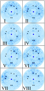
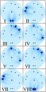
Figure 3: (a) Hybridized trilobite orbitals for a randomly oriented molecular configuration. The Rydberg atom is located at the blue point in the middle of each panel and the neutral atoms are placed at the black points. The common distance $R$ is 1115 a.u. at a local minimum in the lowest energy potential curve. The eigenstates depicted here correspond to APECs that increase in energy from left to right, top to bottom. (b) The same as (a), but in the well the farthest distance from the Rydberg atom at $R=1537$ a.u.

The full APEC results are shown in figure (6), where the exact full diagonalization (black lines) and symmetry-adapted orbital calculation from equations (2.4.2-24) (colored points) are compared. The dispersion between different irreps is clearly observed, as has been previously predicted for smaller systems. [23]. Excellent agreement between the exact and the symmetry-adapted orbital approach is apparent.

3.2 Two-dimensional geometry: random configuration

Molecules that are not configured symmetrically can still be studied via equation (19), and the contrasts between these results and those of highly symmetric configurations are of substantial interest. As an example, the hybridized trilobite orbitals for a co-planar, randomly structured geometry at two Rydberg-neutral internuclear distances are displayed in figure (3). The orbitals at the smaller internuclear distance show substantial interference patterns. Interestingly, for each APEC the electron probability tends to be localized on a subset of the neutral atoms. This subset varies between APECs and is especially clear at the larger internuclear distance displayed in (3b). A possible explanation stems from semi-classical periodic orbit theory, since the trilobite state $\mathbf{\Upsilon_{Rr}^{11}}$ forms due to interference between the four semiclassical elliptical trajectories focused on the Rydberg core and intersecting at both the neutral atom and at the observation point $\vec{r}$ [34]. Since an ellipse focused on the Rydberg core can lie on at most two neutral atoms, this mechanism is a plausible explanation for why these hybridized orbitals tend to be most localized on two neutral atoms. This phenomenon is not seen in highly symmetric molecules, like the octagon of figure (2), since the atoms bound by the Rydberg orbit are here determined by the irrep. An additional feature of these unstructured molecules is that deepest/shallowest well partners, i.e. I and VIII, II and VII, etc. are localized on the same atoms but possess different parity with respect to reflection through the $xy$ plane.

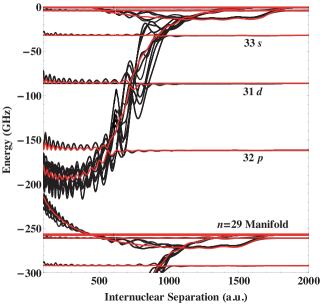
Figure 4: (Color online) APECs for Rydberg states between the $n=29$ and $30$ manifolds for the cubic molecular geometry. The diatomic potential curves are plotted for comparison in red. Large potential wells deep in the butterfly potential curves form, in stark contrast to the diatomic case.

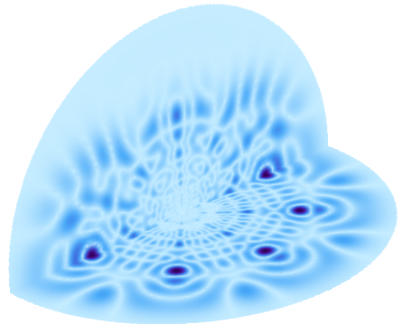
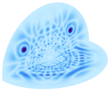
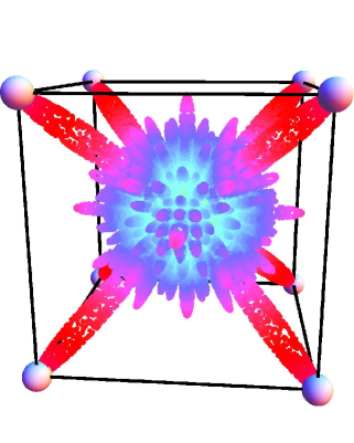
Figure 5: Probability amplitudes cuts in the $xy$ and $yz$ planes for the $A_{1g}$ symmetry species of the trilobite-dominated hybridized orbitals, showing the intricate interference patterns for (a) the octagon and (b) the cube (the $yz$ plane here passes through the diagonal of a face). (c) A polar plot of the $A_{1g}$ cubic hybridized trilobite state: the probability amplitude, scaled to highlight the nodal structure, is plotted as the distance from the center as a function of $\theta$ and $\varphi$.

3.3 Three-dimensional geometry: cubic and asymmetric molecules.

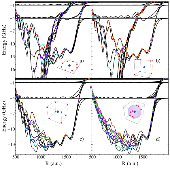
Figure 6: Adiabatic potential energy curves for the breathing mode of a Rydberg-eight neutral atom molecule plotted as a function of the internuclear spacing $R$. In panel (a) the neutral atoms (red spheres in the inset) are restricted to a plane and placed in an octagon; in (b) they are placed in a cube. In (c) the $O_{h}$ symmetry is broken by perturbing the atomic positions randomly by a ten percent deviation, and in (d) it is completely broken by uniformly randomly distributing the ground state atoms in a spherical shell around the Rydberg atom. The $p$-wave interaction is neglected for simplicity in (c) and (d). The colored points in (a) and (b) are the results of equation (24) and in (c) and (d) of equation (19), while the black curves are the result of diagonalization. Disagreements between the analytic and full diagonalization methods are apparent for energies between the $f$ state, with its small but non-zero quantum defect, and the hydrogenic manifold; however, for larger detunings the agreement is excellent.

The exemplary three-dimensional molecule here is a body-centered cubic, which has the highly symmetric point group $O_{h}$, which decomposes into eight total irreps:

$$\Gamma_{O_{h}}^{\text{trilobite}}=A_{1g}\oplus A_{2u}\oplus F_{2u}\oplus F_{1g}$$ (27)

for the trilobite and $R$-butterfly, and

$$\Gamma_{O_{h}}^{\text{butterflies}}=E_{1}\oplus E_{2}\oplus F_{1g}\oplus F_{1u}\oplus F_{2g}\oplus F_{2u}$$ (28)

for the angular butterflies. Figure (5) displays a series of wavefunction images highlighting the three-dimensional structure of these states. The full set of polyatomic APECs between the $n=29$ and $n=30$ manifolds is displayed in figure (4). Compared to the diatomic case, the oscillations in the butterfly states are greatly enhanced, especially near crossings with the low-$l$ states where large wells form, strengthening the binding energies of molecules formed in these wells.

When the neutral atoms are displaced slightly the degeneracy imposed by the $O_{h}$ group is broken, as shown in figure (6(c)) and similarly in figure (6(d)) for randomly placed atoms on a sphere. Only the trilobite state is shown for clarity. In addition to the destruction of the degeneracy and the appearance of avoided crossings, the huge splitting between orbitals of different symmetry seen at $500\leq R\leq 1000$ is reduced.

3.4 Low-$l$ states

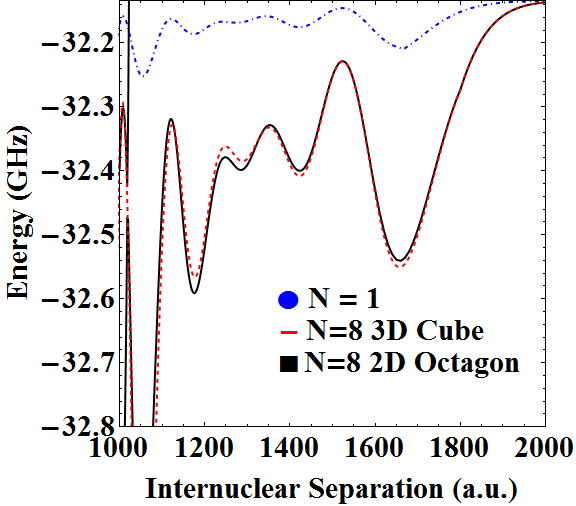
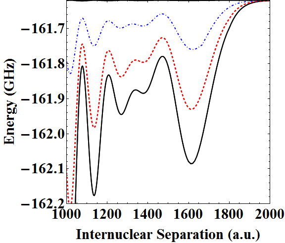
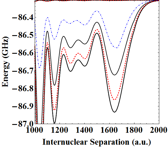
Figure 7: (a) $l=0$, (b) $l=1$, and (c) $l=2$ low angular momentum potential energy curves for $N=1$ (blue curve) and $N=8$, arranged in both a coplanar octagonal geometry (black curves) and a cubic geometry (red curves).

Most experimental probes of these exotic molecules thus far have focused on low-$l$ states. It is increasingly evident [18, 19, 20] that trimers, tetramers, and even pentamers are routinely formed in these experiments, and the results studied here may be relevant in explaining the non-Lorentzian line-shapes of these spectra. Although a full application of these methods to the line-shape would require investigation of the full potential energy surfaces beyond the breathing mode cuts, some conclusions can be made. The $l=0$ results shown in figure (7a) are nearly independent of geometry due to the isotropy of the unperturbed state, and their depths scale linearly with $N$. According to the first order theory in equation (2.3) the well depth for an $N$-atomic molecule is exactly $N$ times the diatomic depth, but due to the couplings with higher-$l$ states the depth of the largest well scales as $\simeq 0.65N$ times the diatomic well depth for the $n=30$ cases studied here. This scaling holds for arbitrary number of atoms and geometries. As such, the appearance of spectral lines at integer multiples of fundamental diatomic lines signifies the production of polyatomic molecules [19]. In contrast, the $l=1$ and $l=2$ states are more complicated as they depend strongly on $N$ and the molecule’s geometry. The spectral signatures of these polyatomic molecules will not be present as individual states, but will instead contribute to line broadening of the diatomic spectrum, and experiments with these states at high densities will need to carefully consider these effects to accurately identify spectral features. The crossover into a density shift [19, 21] will be particularly relevant for these states.

4 The role of density

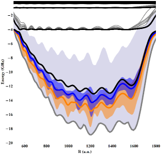
Figure 8: Breathing mode potential curves for the diatomic case (black), the mean (blue curve) and standard deviation (blue envelope) of 100 randomly distributed $N=3$ systems, the mean (orange curve) and standard deviation (orange envelope) of 100 randomly distributed $N=8$ systems, and in gray the potential curves for a $N=30$ system. The overlap between orange and blue shades is denoted by a purple color. For clarity, the thirty different potential curves resulting from this case are represented with the gray envelope extending from the ground state curve to the most shallow.

When the neutral ground state atoms are configured randomly general trends with increasing $N$ can be identified. The ground state APEC for polyatomic molecules with $N=3$, $8$, and $30$ atoms placed on the surface of a sphere of radius $R$ are studied by averaging one hundred different random geometries. The mean value and the standard deviation are presented in figure (8). The well depths increase with $N$ and the position of the minimum is shifted towards smaller distances, compensating for the fact that the electron has to interact with an increasing number of perturbers by drawing them closer where the electron has a semiclassicaly higher kinetic energy. The spreading of the well depths generally increases with $N$. The gray envelope and curve in this figure represent all the APECs for a single thirty-atom case, rather than the mean and standard deviation of one hundred simulations. The overall spread between the ground state and the highest APEC are represented by a single shade for visual clarity.

The results presented in figure (8) are the generalization of the effects seen in the low-$l$ states to trilobite and butterfly states at high density. Both of these results will impact experiments where the shift of the Rydberg excitation energy is employed to estimate the density where the excitation is created [19]. Typically a mean field approach is assumed and the shift of the Rydberg state is related with the average shift of the mean field energy due to the presence of the Rydberg atom in the many-body system. In this picture the shift is independent of the Rydberg state and depends only on the density [17, 35]. However, the findings presented here suggest that the presence of multiple neutrals within the Rydberg orbit will tend to deepen the effective Rydberg-neutral interaction, thus imposing some constraints on the validity of the mean field approach.

5 Conclusions

Calculations elucidating the role of symmetry and geometry in the formation of polyatomic Rydberg molecules at high densities have been presented. and provide a robust framework for studying hybridized trilobite-like molecules. The methodology developed in the present work applies to any geometrical configuration and to high Rydberg states. These represent a significant advance towards understanding spectroscopic results in current experiments that the spectroscopic signatures of polyatomic formation will be challenging to interpret as the results are strongly determined by the molecular geometry and the presence of any symmetries in the atomic orientation. $s$-wave states are nearly independent of the system’s geometry and scale linearly with $N$, but higher angular momenta depend non-trivially on the geometry and number of atoms. These dependencies have profound impacts on the density shifts and line broadening interpretations.

The most significant limitation of the current work is that only the breathing modes are studied where the ground state atoms are all equidistant from the Rydberg core. Although the general principles gleaned from this study will likely apply to other vibrational modes, this is still a highly simplified scenario when contrasted to an ultracold gas where atoms are randomly arrayed at different distances from the Rydberg core. However, this seemingly unrealistic scenario may be achieved by merging the current technology in optical lattices with Rydberg spectroscopy techniques. In particular, tilted optical lattices [36] can be used to generate triply occupied Mott-Insulator states; the usual techniques developed in Rydberg spectroscopy will then lead to the controlled formation of Rydberg trimers, although the position of the atoms in each lattice site will still be random. This randomness can be overcome by employing a rotational optical lattice [37], where the centrifugal force can be used to tailor a more controlled geometry. Indeed, by comparing these results with those from trimers formed in a non-rotating lattice, this method can be applied to further study the influence of the geometry. Another possibility is to use current hexagonal and triangular optical lattice technology [38] with lattice spacing on the order of 400 nm in order to have superior control over the geometry of the Rydberg molecules. To form molecules with this internuclear spacing would require higher Rydberg states on the order of $n=70$, and thus might compromise the spectroscopy of the molecular state; optical lattices with smaller lattice spacings are therefore desirable. Finally, the possibility of optical micro traps [39, 40] has to be taken into account, since these provide opportunities to design very specific arrays of single-atom traps. These traps could be designed to avoid some of the problems caused by the line broadening, and also to emulate the same molecule under very different geometrical considerations.

Appendix A Symmetry-adapted orbitals

A.1 Example

We first present an example of how to calculate one matrix representation of a symmetry operation. The example molecule will have four atoms arranged in a tetrahedron, belonging to the point group $T_{d}$. The atoms are placed equidistant from the Rydberg core at the origin and, in order from $A$ to $D$, at $(\theta,\varphi)$ values $(0,0),(b,0),(b,2\pi/3),(b,4\pi/3)$, where $b=\arccos(-1/3)$. According to equations (10-11) the $\theta,\varphi$ butterfly orbitals are thus parallel to the unit vectors $\sin\theta\hat{z}-\cos\theta\cos\varphi\hat{x}-\cos\theta\sin\varphi\hat{y}$ and $\sin\varphi\hat{x}-\cos\varphi\hat{y}$, respectively. Plugging in the actual values for these angles gives the four unit vectors for both orbitals:

$$\theta:-\hat{x},\frac{\hat{x}}{3}+\frac{2\sqrt{2}}{3}\hat{z},-\frac{\hat{x}}{6}+\frac{\hat{y}}{2\sqrt{3}}+\frac{2\sqrt{2}}{3}\hat{z},-\frac{\hat{x}}{6}-\frac{\hat{y}}{2\sqrt{3}}+\frac{2\sqrt{2}}{3}\hat{z}.$$

$$\varphi:-\hat{y},-\hat{y},\frac{\sqrt{3}}{2}\hat{x}+\frac{\hat{y}}{2},-\frac{\sqrt{3}}{2}\hat{x}+\frac{\hat{y}}{2}.$$

As the example symmetry operation we choose one of the $C_{3}$ operations corresponding to a rotation about the $z$ axis by $\frac{2\pi}{3}$ radians. This cyclically rotates the three atomic labels not along the $z$ axis, so that the symmetry operation for the trilobite orbital is

$$\begin{pmatrix}\psi_{A}\\ \psi_{C}\\ \psi_{D}\\ \psi_{B}\end{pmatrix}=\begin{pmatrix}1&0&0&0\\ 0&0&1&0\\ 0&0&0&1\\ 0&1&0&0\end{pmatrix}\begin{pmatrix}\psi_{A}\\ \psi_{B}\\ \psi_{C}\\ \psi_{D}\end{pmatrix}.$$

The rotation matrix in coordinate space corresponding to this symmetry operation is

$$\begin{pmatrix}-\frac{1}{2}&-\frac{\sqrt{3}}{2}&0\\ \frac{\sqrt{3}}{2}&-\frac{1}{2}&0\\ 0&0&1\end{pmatrix}$$ (29)

which then must act on the orbitals. For example the $\theta$ orbital originally at $A$, $-\hat{x}$, is rotated to become:

$$\begin{pmatrix}\frac{1}{2}\\ \frac{\sqrt{3}}{2}\\ 0\end{pmatrix}=\begin{pmatrix}-\frac{1}{2}&-\frac{\sqrt{3}}{2}&0\\ \frac{\sqrt{3}}{2}&-\frac{1}{2}&0\\ 0&0&1\end{pmatrix}\begin{pmatrix}-1\\ 0\\ 0\end{pmatrix}.$$ (30)

The linear combination of $\theta$ and $\varphi$ butterfly orbitals at $A$ that equals $(\frac{1}{2},-\frac{\sqrt{3}}{2},0)^{T}$ are then solved, giving

$$(\psi^{\theta}_{A})^{\prime}=-\frac{1}{2}\psi^{\theta}_{A}+\frac{\sqrt{3}}{2}\psi^{\varphi}_{B}.$$ (31)

Likewise, the rotation matrix acting on the orbital $\psi^{\theta}_{B}$ rotates it to:

$$\begin{pmatrix}-\frac{1}{6}\\ \frac{1}{2\sqrt{3}}\\ \frac{2\sqrt{2}}{3}\end{pmatrix}=\begin{pmatrix}-\frac{1}{2}&-\frac{\sqrt{3}}{2}&0\\ \frac{\sqrt{3}}{2}&-\frac{1}{2}&0\\ 0&0&1\end{pmatrix}\begin{pmatrix}\frac{1}{3}\\ 0\\ \frac{2\sqrt{2}}{3}\end{pmatrix}.$$ (32)

The resultant vector is identified as the $\theta$ orbital at $C$, so the permutation of labels was sufficient here and there is no mixing of angular butterfly orbitals. In the end, the enlarged symmetry operation matrix is

$$\begin{pmatrix}-\frac{1}{2}&0&0&0&\frac{\sqrt{3}}{2}&0&0&0\\ 0&0&1&0&0&0&0&0\\ 0&0&0&1&0&0&0&0\\ 0&1&0&0&0&0&0&0\\ -\frac{\sqrt{3}}{2}&0&0&0&-\frac{1}{2}&0&0&0\\ 0&0&0&0&0&0&1&0\\ 0&0&0&0&0&0&0&1\\ 0&0&0&0&0&1&0&0\end{pmatrix}.$$ (33)

The presence of negative or fractional values on the diagonals is what contributes to the trace of $\hat{P}^{j}$, giving different decompositions.

A.2 SAO coefficients

The coefficients $\mathcal{A}_{p}^{(j,\alpha)}$ are given here for the example symmetries. The rows of each matrix correspond to a given irrep $j$ labeled in the first column; each column thereafter corresponds to a diatomic orbital at $\vec{R}_{p}$. For the octagon the labeling simply proceeds around the octagon; the first four columns of the cube correspond to the upper layer ordered counter-clockwise viewed from above; the final four correspond to the bottom layer ordered identically.

A.3 Octagon

$$\mathbf{\mathcal{A}^{1,2,3}_{C_{8v}}} =\left(\begin{array}[]{ccccccccc}A_{1}&1&1&1&1&1&1&1&1\\ B_{2}&1&-1&1&-1&1&-1&1&-1\\ E_{1}&1&a&1&0&-1&-a&-1&0\\ E_{1}&-1&0&1&a&1&0&-1&-a\\ E_{2}&1&0&-1&0&1&0&-1&0\\ E_{2}&0&1&0&-1&0&1&0&-1\\ E_{3}&-1&a&-1&0&1&-a&1&0\\ E_{3}&-1&0&1&-a&1&0&-1&a\end{array}\right)$$

$$\mathbf{\mathcal{A}^{4}_{C_{8v}}} =\left(\begin{array}[]{ccccccccc}A_{2}&1&1&1&1&1&1&1&1\\ B_{1}&1&-1&1&-1&1&-1&1&-1\\ E_{1}&-1&0&1&a&1&0&-1&-a\\ E_{1}&1&a&1&0&-1&-a&-1&0\\ E_{2}&0&1&0&-1&0&1&0&-1\\ E_{2}&1&0&-1&0&1&0&-1&0\\ E_{3}&-1&0&1&-a&1&0&-1&a\\ E_{3}&-1&a&-1&0&1&-a&1&0\end{array}\right),$$

$a=\sqrt{2}$. As described in section (3.1) the $\theta$-butterfly is decoupled for all co-planar molecules.

A.4 Cube

$$\mathbf{A_{O_{h}}^{1,2}} =\left(\begin{array}[]{ccccccccc}A_{1g}&1&1&1&1&1&1&1&1\\ A_{2u}&1&-1&1&-1&-1&1&-1&1\\ F_{1u}&1&-1&1&-1&1&-1&1&-1\\ F_{1u}&-1&0&1&0&1&0&-1&0\\ F_{1u}&0&1&0&-1&0&-1&0&1\\ F_{2g}&1&1&1&1&-1&-1&-1&-1\\ F_{2g}&0&-1&0&1&0&-1&0&1\\ F_{2g}&1&0&-1&0&1&0&-1&0\end{array}\right)$$

$$\mathbf{A_{O_{h}}^{3}} =\left(\begin{array}[]{ccccccccc}E_{1}&1&1&1&1&-1&-1&-1&-1\\ E_{1}&0&0&0&0&0&0&0&0\\ E_{2}&1&-1&1&-1&1&-1&1&-1\\ E_{2}&0&0&0&0&0&0&0&0\\ F_{1g}&b&0&-b&0&b&0&-b&0\\ F_{1g}&0&b&0&-b&0&b&-b&0\\ F_{1g}&0&0&0&0&0&0&0&0\\ F_{1u}&1&1&1&1&1&1&1&1\\ F_{1u}&0&-1&0&1&0&1&0&-1\\ F_{1u}&1&0&-1&0&-1&0&1&0\\ F_{2g}&1&-1&1&-1&-1&1&-1&1\\ F_{2g}&-1&0&1&0&-1&0&1&0\\ F_{2g}&0&1&0&-1&0&1&0&-1\\ F_{2u}&b&0&-b&0&-b&0&b&0\\ F_{2u}&0&b&0&-b&0&-b&0&b\\ F_{2u}&0&0&0&0&0&0&0&0\end{array}\right)$$

$$\mathbf{A_{O_{h}}^{4}} =\left(\begin{array}[]{ccccccccc}E_{1}&0&0&0&0&0&0&0&0\\ E_{1}&1&1&1&1&-1&-1&-1&-1\\ E_{2}&0&0&0&0&0&0&0&0\\ E_{2}&1&-1&1&-1&1&-1&1&-1\\ F_{1g}&0&1&0&-1&0&-1&0&1\\ F_{1g}&1&0&-1&0&1&0&-1&0\\ F_{1g}&1&0&-1&0&1&0&-1&0\\ F_{1u}&0&0&0&0&0&0&0&0\\ F_{1u}&b&0&-b&0&b&0&-b&0\\ F_{1u}&0&b&0&-b&0&b&0&-b\\ F_{2g}&0&0&0&0&0&0&0&0\\ F_{2g}&0&b&0&-b&0&-b&0&b\\ F_{2g}&b&0&-b&0&-b&0&b&0\\ F_{2u}&0&-1&0&1&0&-1&0&1\\ F_{2u}&1&0&-1&-0&1&0&-1&0\\ F_{2u}&1&-1&1&-1&-1&1&-1&1\end{array}\right),$$

$b=\sqrt{3}$.

References

References

- [1] Greene C H, Dickinson A S and Sadeghpour H R 2000 Phys. Rev. Lett. 85, 2458
- [2] Hamilton E L, Greene C H and Sadeghpour H R 2002 J. Phys. B 35, L199
- [3] Hamilton E L 2002, Ph.D. thesis, University of Colorado
- [4] Khuskivadze A A, Chibisov M I and Fabrikant I I 2002 Phys. Rev. A 66, 042709; Chibisov M I, Khuskivadze A A, and Fabrikant I I 2002 J. Phys. B 35, L193
- [5] Li W, Pohl T, Rost J M, Rittenhouse S T, Sadeghpour H R, Nipper J, Butscher B, Balewski J B, Bendkowsky V, Löw R and Pfau T 2011 Science 334, 1110
- [6] Bendkowsky V, Butscher B, Nipper J, Balewski J B, Shaffer J P, Löw R and Pfau T 2009 Nature (London) 458 1005
- [7] Saßmannshausen H, Merkt F, and Deiglmayr J 2014 Phys. Rev. Lett. 114, 133201
- [8] Anderson D A, Miller S A and Raithel G 2014 Phys. Rev. Lett. 112, 163201
- [9] Krupp A T, Gaj A, Balewski J B, Ilzhöfer P, Hofferberth S, Löw R, Pfau T, Kurz M and Schmelcher P 2014 Phys. Rev. Lett. 112, 143008
- [10] Gaj A, Krupp A T, Ilzhöfer P, Löw R, Hofferberth S and Pfau T Phys. Rev. Lett. 115, 023001
- [11] Booth D, Rittenhouse S T, Yang J, Sadeghpour H R, & Shaffer J P 2015 Science, 348, 99.
- [12] Manthey T, Niederprüm, and Ott H 2015 New J. Phys. 17 103024.
- [13] Eiles M T and Greene C H 2015 Phys. Rev. Lett. 115, 193201
- [14] DeSalvo B J, Aman J A, Dunning F B, Killian T C, Sadeghpour H R, Yoshida S, and Burgdörfer J 2015 Phys. Rev. A 92, 031403(R)
- [15] Bendkowsky V, Butscher B, Nipper J, Balewski J B, Shaffer J P, Löw R, Pfau T, Li W, Stanojevic J, Pohl T and Rost J M 2010 Phys. Rev. Lett. 105, 163201
- [16] Böttcher F, Gaj A, Westphal K M, Schlagmüller M, Kleinbach K S, Löw R, Liebisch T C, Pfau T, Hofferberth S 2015 arXiv:1510.01097
- [17] Balewski J B, Krupp A T, Gaj A, Peter D, Büchler H P, Löw R, Hofferberth S and Pfau T (2013) Nature (London) 502, 664
- [18] Karpiuk T, Brewczyk M, Rzazewski K, Gaj A, Balewski J B, Krupp A T, Schlagmüller M, Löw R, Hofferberth S, Pfau T 2015 New J. Phys, 17 5 053046
- [19] Gaj A, Krupp A T, Balewski J B, Löw R, Hofferberth S and Pfau T 2014 Nat. Commun. 5, 4546
- [20] Schlagmüller M, Liebhisch T C, Nguyen H, Lochead G, Engel F, Böttcher F, Westphal K M, Kleinbach K S, Löw R, Hofferberth S, Pfau T, Pérez-Ríos J, Greene C H 2015 arXiv:1510.07003
- [21] Schmidt R, Sadeghpour H R and Demler E 2015 arXiv:1510.09183v1
- [22] Liu I C H, Stanojevic J and Rost J M 2009 Phys. Rev. Lett. 102, 173001
- [23] Liu I C H and Rost J M 2006 Eur. Phys. J. D 40, 65
- [24] Fernández J A, Schmelcher P, and González-Férez 2016 arXiv:1601.05049
- [25] Bunker P R and Jensen P 1998, Molecular symmetry and spectroscopy. NRC Research Press, Ottawa
- [26] Bunker P R and Jensen P 2004, Fundamentals of molecular symmetry CRC Press, Series in Chemical Physics
- [27] Fermi E 1934 Nuovo Cimento 11, 157
- [28] Omont A 1997, J. Phys. (Paris) 38, 1343
- [29] Bahrim Cand Thumm U 2000 Phys. Rev. A 61 022722
- [30] Fey C, Kurz M, Schmelcher P, Rittenhouse S T and Sadeghpour H R 2015 New J. Phys. 17 055010
- [31] Chibisov M, Ermolaev A M, Brouillard F, and Cherkani M H 2000 Phys. Rev. Lett. 84, 45; see also Cherkani M H, Brouillard F, and Chibisov M 2001 J. Phys. B. 34 49.
- [32] Kurz M 2014, Ph.D. Thesis, Hamburg University.
- [33] Bendkowksy V, Butscher B, Nipper J, Balewksi J B, Shaffer J P, Löw R, Pfau T, Li W, Stanojevic J, Pohl T, and Rost J M 2010, Phys. Rev. Lett. 105 163201.
- [34] Granger B, Hamilton E L and Greene C H 2001, Phys. Rev. A 64 042508.
- [35] Wang J, Gacesa M and Côté R 2015, Phys. Rev. Lett. 114 243003.
- [36] Ma R, Tai E M, Preiss PM, Bakr W S, Simon J, Greiner M 2011 Phys. Rev. Lett. 107, 095301
- [37] Williams R A, Al-Assam S, Foot CJ 2010 Phys. Rev. Lett. 104, 050404
- [38] Lühmann D-S, Jürgensen O, Weinberg M, Simonet J, Soltan-Panahi P, Sengstock, K 2012 Phys. Rev. A 90, 013614
- [39] Henderson K, Ryu C, MacCormick C, Boshier MG 2009 New J. Phys. 11, 043030
- [40] Zimmermann B, T Müller T, Meineke J, Esslinger T, Moritz, H 2011 New J. Phys. 13, 043007