Molecular Distribution in the Spiral Arm of M51

Abstract

Molecular line images of ¹³CO, C¹⁸O, CN, CS, CH₃OH, and HNCO are obtained toward the spiral arm of M51 at a $7^{\prime\prime}\times 6^{\prime\prime}$ resolution with the Combined Array for Research in Millimeter-wave Astronomy (CARMA). Distributions of the molecules averaged over a 300 pc scale are found to be almost similar to one another and to essentially trace the spiral arm. However, the principal component analysis shows a slight difference of distributions among molecular species particularly for CH₃OH and HNCO. These two species do not correlate well with star-formation rate, implying that they are not enhanced by local star-formation activities but by galactic-scale phenomena such as spiral shocks. Furthermore, the distribution of HNCO and CH₃OH are found to be slightly different, whose origin deserves further investigation. The present results provide us with an important clue to understanding the 300 pc scale chemical composition in the spiral arm and its relation to galactic-scale dynamics.

1 Introduction

Recently, various molecular species have readily been detected in nearby galaxies owing to rapid improvements in sensitivities of radioastronomical observations, and chemistry of molecular gas in external galaxies has attracted more attention of astronomers than before. So far, about 60 molecular species have been identified in external galaxies. Chemical studies for external galaxies have mostly been focused on nuclear regions, which usually give bright molecular emissions. Spectral line surveys have extensively been conducted in such regions to characterize chemical nature of molecular gas (e.g. Martín et al., 2006; Aladro et al., 2011, 2013, 2015; Costagliola et al., 2011; Nakajima et al., 2011; Snell et al., 2011). Distributions of various molecular species around the nuclear regions have been revealed with radio interferometers such as ALMA, and they are used to investigate peculiar physical states of the nuclear regions (e.g. Izumi et al., 2013; Sakamoto et al., 2014; Takano et al., 2014; Meier et al., 2015; Martín et al., 2015; Nakajima et al., 2015).

On the other hand, there are relatively few chemical studies in disk regions of external galaxies, because intensities of molecular line emissions are usually much weaker there than in the galactic nuclei. Meier & Turner (2005, 2012) imaged distributions of about 10 molecular species in the nuclear and bar regions of IC 342 and Maffei 2 with the OVRO and BIMA, and revealed significant chemical differentiation among giant molecular clouds (GMCs). For instance, CH₃OH, HNCO, and SiO are enhanced in the bar region. They concluded that large-scale shocks induced by gas dynamics specific to the bar structure are responsible to the enhancements. However, chemical compositions observed toward external galaxies are those averaged over one or more GMCs within a telescope beam. Therefore, we need to pay particular attention to this point, when we discuss chemical compositions of external galaxies on the basis of astrochemical concepts established for sub-pc scale regions in Galactic molecular clouds. For instance, chemical evolutionary effects (e.g. Suzuki et al., 1992), which are important for sub-pc scale clouds, may not be very important in the GMC-scale chemical compositions, because the time scale of the chemical equilibrium (10⁶ yr) is much shorter than the sound crossing time of GMCs ($>10^{7}$ yr). Hence, it seems likely that the GMC-scale chemical compositions are more or less in chemical equilibrium, and mainly depend on structures and environmental conditions of GMCs. For better understanding of chemical effects in starbursts, AGNs, and shocks in spiral arms and bar regions, we need to establish the ‘standard’ chemical composition of GMCs without or almost without these specific effects. With this motivation, we have been studying the chemical composition in the spiral arm region of M51 (Watanabe et al., 2014).

M51 is a grand-design spiral galaxy located at the distance of 8.4 Mpc (Feldmeier et al., 1997; Vinkó et al., 2012). The distribution and dynamics of molecular gas in this galaxy have extensively been studied using both single dish telescopes (Nakai et al., 1994; Schuster et al., 2007; Kuno et al., 2007; Miyamoto et al., 2014) and interferometers (Aalto et al., 1999; Helfer et al., 2003; Koda et al., 2009; Schinnerer et al., 2013). Spectral line survey observations have been conducted toward two positions in the spiral arm in the 2 mm and 3 mm bands (Watanabe et al., 2014) as well as the nuclear region in the 3 mm band (Aladro et al., 2015). The spectral pattern observed in the two positions (P1 and P2) were very similar to each other indicating similar chemical compositions, although the one (P1) shows higher star formation activity than the other (P2). Toward the P1 position, 15 molecular species have been identified. The spectrum pattern is much different from that reported for high-mass star forming regions such as Orion KL (e.g. Tercero et al., 2010; Watanabe et al., 2015), indicating that the observed chemical composition cannot simply be interpreted in terms of a composite of contributions from embedded star forming cores. The GMC-scale distribution of molecules would mainly contribute to the spectrum. Indeed, we detected the cold dense gas tracer N₂H⁺ in our observation toward M51, which is relatively weak in high-mass star forming regions (Watanabe et al., 2015). Assuming optically thin and local thermodynamic equilibrium (LTE) conditions, the excitation temperatures of CS, HNCO, and CH₃OH are estimated to be less than 10 K in M51 P1. This result indicates that most of detected molecules reside in a cold ($\sim 10$ K) and widespread molecular gas, although a part of the molecular emission may also come from the hot molecular gas, e.g. hot cores affected by the feedbacks from star formation activities.

However, the resolution of our previous line-survey observation is about $30^{\prime\prime}$, which corresponds to the linear scale of 1 kpc. High angular resolution observations are needed to explore the origin and the nature of the molecular emission in more detail. In this study, we imaged the 6 molecular species in the spiral arm of M51 with the Combined Array for Research in Millimeter-wave Astronomy (CARMA).

2 Observations with CARMA

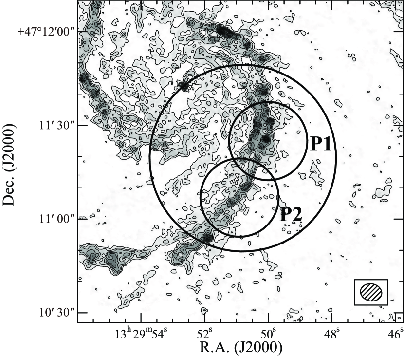
Figure 1: A field of view of the observation with the CARMA (large circle) superposed on contours of the CO integrated intensity (PAWS: Schinnerer et al., 2013). Small circles indicate the beam size ($25^{\prime\prime}$) of the IRAM 30 m telescope at the 100 GHz toward the P1 and P2 positions (Watanabe et al., 2014). A hatched ellipse indicates a synthesized beam ($6.9^{\prime\prime}\times 5.5^{\prime\prime}$ with the position angle of $79.9^{\circ}$) of the CARMA observation at the 97 GHz.

The observations were carried out with the CARMA in May and June 2014. It consists of six 10.4 m and nine 6.1 m antennas. The primary beams of the 10.4 m and 6.1 m antennas at 110 GHz are about $60^{\prime\prime}$ and $100^{\prime\prime}$, respectively. The phase-center coordinate is : (R. A., Dec.) = (13:29:50.8, +47:11:19.5) in J2000 (Figure 1). Six molecular species, ¹³CO, C¹⁸O, CN, CH₃OH, HNCO, and CS (Table 1), were simultaneously observed in the array configuration of D and E. These configurations cover a baseline range of $\sim 2-55$ k$\lambda$. The system noise temperatures were about 160–380 K. The CH₃OH and CS lines and the C¹⁸O, HNCO, ¹³CO, and CN lines were observed in the lower sideband and the upper sideband, respectively. We employed 6 correlators for the 6 molecular lines. The bandwidth of each correlator is 125 MHz with a frequency resolution of 0.781 MHz. The bandpass calibration was done with the radio sources 3C273 and 3C279. 1419+543 was observed for 3 minutes every 15 minutes as a phase and gain calibrator. The absolute flux of 1419+543 was measured by comparing with the flux of Mars. The uncertainty of flux calibration is 20 %. The data reduction and analysis were done by using the MIRIAD package. The synthesized beam size and the root-mean-square (r. m. s.) noise level of each molecule are summarized in Table 1. In the imaging procedure, the spectral channels were regrided. The final velocity resolutions are summarized in Table 1.

3 Results

3.1 Overview of molecules

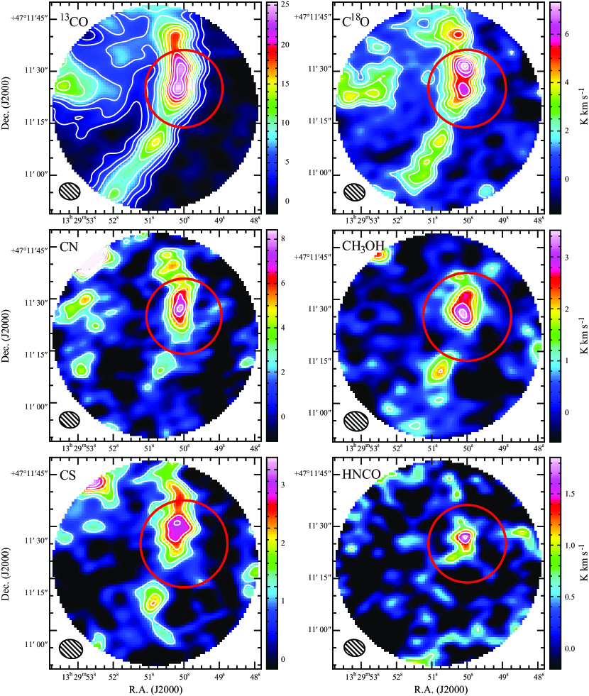
Figure 2: Integrated intensity maps of ¹³CO, C¹⁸O, CN, CH₃OH, CS, and HNCO. The synthesized beams are shown as ellipticals in the lower left corner. The red circles indicate the beam size of the IRAM 30 m telescope at P1. Contour levels of the ¹³CO integrated intensity are 0.7 K km s${}^{-1}\times(3,6,9,12,15,18,21,24,27,30,33)$. Contour levels of the C¹⁸O integrated intensity are 0.7 K km s${}^{-1}\times(2,3,4,5,6,7,8,9,10)$. Contour levels of the CN integrated intensity are 1.1 K km s${}^{-1}\times(2,3,4,5,6,7)$. Contour levels of the CH₃OH integrated intensity are 0.55 K km s${}^{-1}\times(2,3,4,5,6)$. Contour levels of the CS integrated intensity are 0.40 K km s${}^{-1}\times(2,3,4,5,6,7)$. Contour levels of the HNCO integrated intensity are 0.35 K km s${}^{-1}\times(2,3,4,5)$.

The ¹³CO ($J=1-0$), C¹⁸O ($J=1-0$), CN ($N=1-0$), CH₃OH($J=2_{\rm k}-1_{\rm k}$), HNCO($5_{0\,5}-4_{0\,4}$), and CS($J=2-1$) lines were successfully detected. Figure 2 shows integrated intensity maps of the 6 molecular species. A primary beam correction was applied to these maps. The ¹³CO emission is found to be widely distributed along the spiral arm, nuclear bar, and molecular ring regions, which are defined by Hughes et al. (2013). Our ¹³CO($J=1-0$) map is similar to the ¹³CO($J=1-0$) map observed with the Owens Valley Radio Observatory mm-interferometer (Schinnerer et al., 2010), although the synthesized beam size of our map is coarser than their map (2.9^′′). Since the intensity of the ¹³CO line is the strongest among the 6 molecules and the critical density is as low as $10^{3}$ cm^-3, this line would trace an entire distribution of molecular gas including relatively diffuse gas which cannot be traced by the other lines with higher critical densities. The distribution of C¹⁸O is more clumpy than that of ¹³CO. The C¹⁸O emission traces higher column-density regions, because the optical depth of the C¹⁸O line is generally thinner than the ¹³CO line.

Critical densities of the CN, CH₃OH, HNCO, and CS lines ($\sim 10^{5}$ cm^-3) are much higher than those of the ¹³CO and C¹⁸O lines, and hence, these lines tend to trace denser molecular gas than the CO isotopologue lines. The CN emission is detected along the spiral arm and shows a strong peak at the P1 position. The CN distribution is extended from the CN peak to the northern direction. The CS emission is also distributed along the spiral arm, and extends to the northern direction from the peak at the P1 position. On the other hand, CH₃OH shows a rather compact distribution without any extended structures toward the northern direction from the peak at the P1. HNCO shows a single peak at the P1 position probably due to an insufficient sensitivity of this observation. The HNCO peak coincides with the CH₃OH peak. Although the distributions of all the molecules are along the spiral arm, we recognize a slight variation among molecular species.

3.2 Missing flux

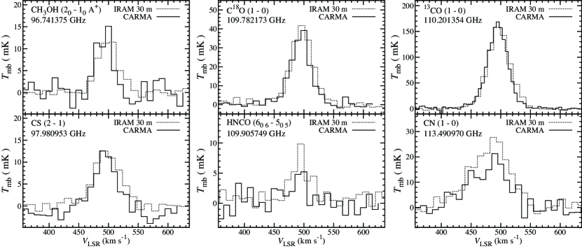
Figure 3: Spectral line profiles observed toward the M51 P1 with the CARMA (solid line) and the IRAM 30 m telescope (dotted line: Watanabe et al., 2014). The CARMA spectra are prepared by convolving the cleaned map by the resolution of the CH₃OH map.

Missing fluxes in the CARMA observations are evaluated by comparing with the fluxes obtained with the IRAM 30 m telescope (Watanabe et al., 2014). The angular resolution of the CARMA maps are adjusted by convolving the Gaussian beam to match the beam size of the IRAM 30 m telescope. The convolution is carried out by using a task convol of the MIRIAD software package. The angular resolution of the IRAM 30 m observation for each molecular line is summarized in Table 2. Figure 3 shows the spectra of CH₃OH, CS, C¹⁸O, HNCO, ¹³CO, and CN toward M51 P1 prepared by convolving the CARMA data and the corresponding spectra obtained with the IRAM 30 m telescope. The spectral profile and intensity of the convolved spectrum is similar to the single dish spectrum for each molecule, although the spectral lines of HNCO and CN obtained with CARMA are significantly weaker than those with the IRAM 30 m telescope. The integrated intensities of the both observations are shown in Table 2. If uncertainties of intensity calibrations (20 % both for the IRAM 30 m observations and the CARMA observations) are taken into account, most of fluxes are recovered in the CARMA observation, except for CN and HNCO. As for HNCO, the missing flux is probably due to the poor S/N ratio in the CARMA observation. On the other hand, the missing flux of CN, which is estimated to be 42 %, is puzzling. Since the missing flux of ¹³CO is small, this implies that CN is more extended than ¹³CO. Weak CN emission extended outside the arm region may be resolved out in the CARMA observation. Although we cannot in principle rule out the possibility that the missing flux of CN just originates from imperfect calibration, this possibility is unlikely, because the missing flux of most of molecules are negligible. In any case, the CN abundances estimated in the latter sections tend to be lower than that estimated in Watanabe et al. (2014).

3.3 Spectra at C¹⁸O peaks

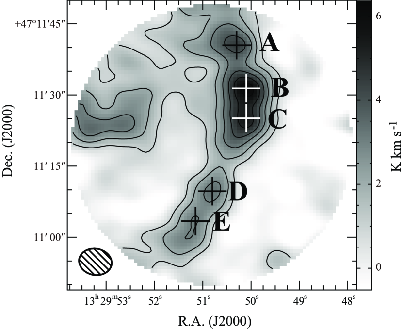
Figure 4: Positions of the C¹⁸O peaks (cross marks) superposed on the C¹⁸O integrated intensity map. Contour levels are 0.5 K km s${}^{-1}\times(2,4,6,8,10,12)$. The angular resolution of the C¹⁸O map is set to be the same as that of the CH₃OH map by convolution.

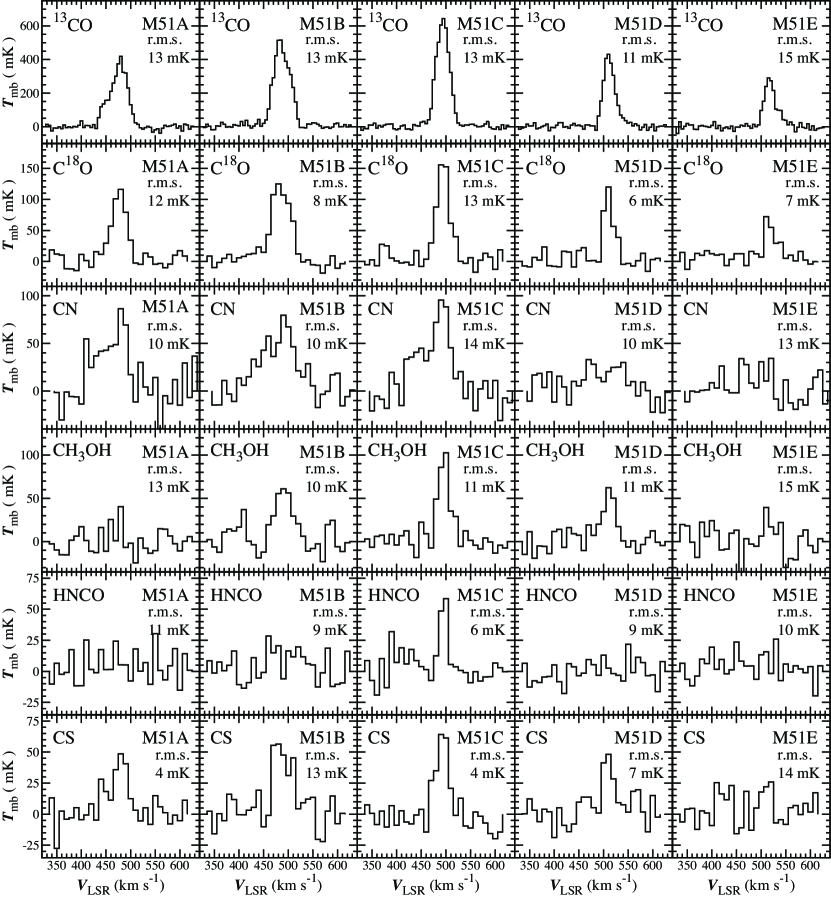
Figure 5: Spectra of the 6 molecules sampled at the 5 C¹⁸O peak positions (Table 3). The spectra are obtained after the spatial resolution is converted to the resolution of the CH₃OH map ($6.0^{\prime\prime}\times 6.9^{\prime\prime}$ with the position angle of $79.9^{\circ}$), which is the beam size of the CH₃OH map. The angular resolution of CH₃OH map is used as the reference resolution, since the angular resolution is the coarsest. The intensity scale is the main beam temperature.

Spectral line parameters are derived for the five peaks of the C¹⁸O integrated intensity (Figure 4 and Table 3), because the C¹⁸O peaks coincide with most of the other molecular line peaks and likely represent association of GMCs. In order to compare the spectra at the same angular resolution, the ¹³CO, C¹⁸O, CN, CS, and HNCO maps are convolved with the Gaussian beam for the CH₃OH map ($6.9^{\prime\prime}\times 5.5^{\prime\prime}$) by using the MIRIAD task convol. The angular resolution of the final maps is thus the same as that of CH₃OH. Figure 5 shows the spectra obtained at the five C¹⁸O peaks. Table 4 summarizes peak intensities, integrated intensities, line-of-sight velocities, and line widths of the spectra. In the case of non-detection, the $3\sigma$ upper limits to the peak temperature and the integrated intensity are given. The line profiles of CN are different from those of the other molecules, because four hyperfine lines are blended. Therefore, the linewidths and the line-of-sight velocities are not evaluated for the CN lines.

3.4 Molecular abundances

Beam-averaged column densities of ¹³CO, C¹⁸O, CN, CH₃OH, HNCO, and CS are evaluated for the C¹⁸O peak positions (Table 3), under the LTE assumption by using the following formula:

$$W_{\nu}=\frac{8\pi^{3}S\mu_{0}^{2}\nu N}{3kU(T_{\rm rot})}\left\{1-\frac{\exp(h\nu/kT_{\rm rot})-1}{\exp(h\nu/kT_{\rm bg})-1}\right\}\exp\left(-\frac{E_{\rm u}}{kT_{\rm rot}}\right),$$ (1)

where $W_{\nu}$, $S$, $\mu_{0}$, $\nu$, $N$, $k$, $T_{\rm rot}$, $U(T_{\rm rot})$, $h$, $T_{\rm bg}$, and $E_{\rm u}$ are integrated intensity, line strength, dipole moment, transition frequency, total column density, the Boltzmann constant, rotation temperature, partition function, the Planck constant, the cosmic microwave background temperature, and upper state energy, respectively. The rotation temperature is assumed to be 10 K on the basis of the single dish result for a few molecules (Watanabe et al., 2014). Since the beam sizes of all molecular data are the same as that of CH₃OH (see Section 3.3), a correction of a beam filling factor is not applied for each molecular line. Hence, these column densities are ones averaged over the $6.0^{\prime\prime}\times 6.9^{\prime\prime}$ scale. The result is summarised in Table 5, and the errors are estimated from the rms noise of the spectrum and the calibration uncertainty (20 %). The column densities are sensitive to the assumed rotation temperature. When we assume the rotation temperature of 5 K and 20 K, the derived column densities vary by factor of 3 and 2, respectively, for the largest cases. In the following analyses, we discuss the fractional abundances relative to H₂ instead of the column densities in order to mitigate the systematic errors caused by the assumption of the rotation temperature.

Fractional abundances relative to H₂ are derived for the C¹⁸O peak positions by using H₂ column densities estimated from C¹⁸O, where the [H₂]/[C¹⁸O] ratio of $2.9\times 10^{6}$ is assumed (Meier & Turner, 2005). The fractional abundances are summarised in Table 6. They are less affected by the assumed rotation temperature than the column densities. Indeed, a difference of the fractional abundance is estimated to be at most within a factor of 2 for the rotation temperature range from 5 K to 20 K, where the maximum case is for HNCO.

4 Discussion

4.1 Principal component analysis

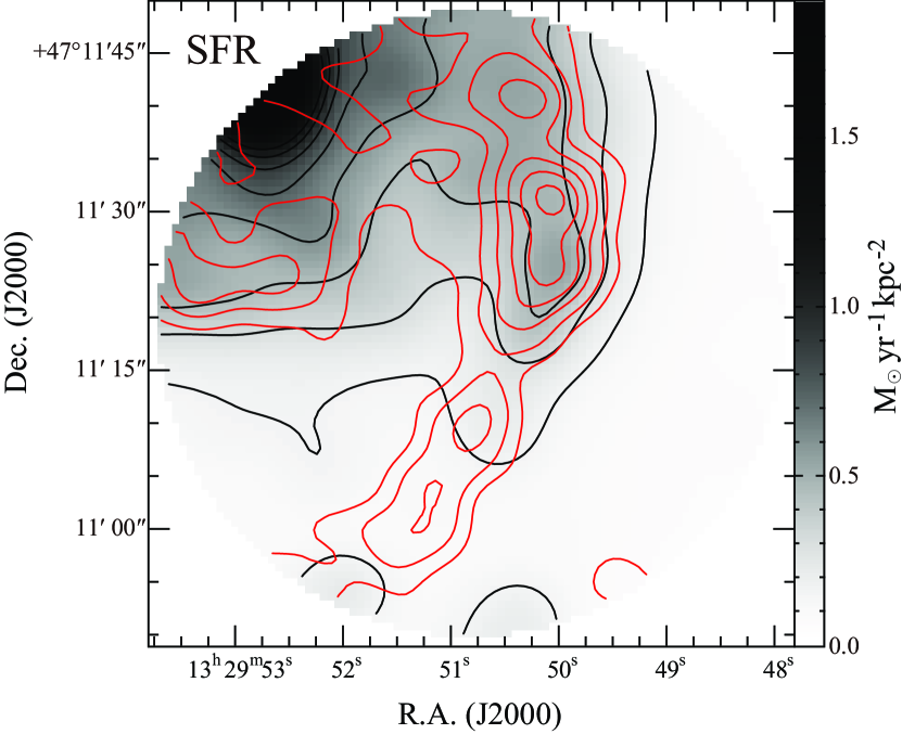
Figure 6: A SFR map (gray scale and black contours) and an integrated intensity map of C¹⁸O (red contours). Contour levels are 0.15 M_⊙yr^-1kpc${}^{-2}\times(1,2,...,8)$ and 0.5 K km s${}^{-1}\times(2,4,...,12)$ for the SFR and the C¹⁸O integrated intensity, respectively. The angular resolutions of the two maps are convolved to the resolution of the CH₃OH map ($6.0^{\prime\prime}\times 6.9^{\prime\prime}$ with the position angle of $79.9^{\circ}$).

We conduct a principal-component analysis (PCA) to evaluate similarity and difference among maps of different molecular lines quantitatively. The PCA has been used as a common analytical technique to quantify morphological correlation of molecular distributions in molecular clouds and external galaxies (e.g. Ungerechts et al., 1997; Meier & Turner, 2005). In addition to the molecular distributions obtained with the CARMA, a surface density distribution of the star-formation rate (SFR) is included in the PCA. The SFR is estimated from the intensities of the H$\alpha$ and 24 $\mu$m emission observed by Kennicutt et al. (2003). In order to compare the SFR map with our molecular maps, the angular resolutions of the H$\alpha$ and 24 $\mu$m maps are convolved to be the resolution of the CH₃OH map. After the convolution, the SFR is evaluated by using the method given by Calzetti et al. (2007), as shown in Figure 6. We used ${\rm SFR}(M_{\odot}\,{\rm yr}^{-1})=5.3\times 10^{-42}[L({\rm H\alpha})_{\rm obs}+(0.031\pm 0.006)\times L({\rm 24\,\mu m})]$, where $L({\rm H\alpha})_{\rm obs}$ and $L({\rm 24\,\mu m})$ are observed luminosities of H$\alpha$ and 24 $\mu$m in erg s^-1, respectively.

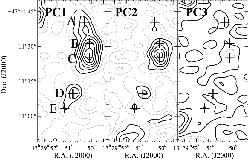
Figure 7: Maps of the first, second, and third principal components. The black contours and dashed contours indicate positive and negative values, respectively.

The PCA is conducted in the same way as Meier & Turner (2005) reported. The molecular line maps are convolved and re-gridded to the same angular resolution for the CH₃OH emission. Then, the pixel values of the molecular maps and the SFR are normalized and mean-centered (Appendix A). After these preprocesses, a correlation matrix is calculated from the preprocessed maps, and its eigenvalues and eigenvectors are then calculated by diagonalizing the correlation matrix. Tables 7 and 8 show the correlation matrix and the eigenvectors, respectively. Figure 7 shows the maps of the first, second and third principal components.

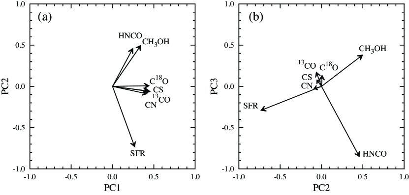
Figure 8: The projection of each molecule on (a) PC1–PC2 and (b) PC2–PC3 planes. The meanings of PC1, PC2, and PC3 are explained in Section 4.1.

Figure 8 shows projection of each species on the first, second, and third PC axes. On the first principal component (PC1) axis, all the species have positive projections with a similar magnitude (0.24–0.45). Hence, the PC1 represents an averaged distribution of molecules and SFR, which essentially traces the spiral arm structure (Figure 7). On the second and third principal component (PC2 and PC3, respectively) axes, ¹³CO, C¹⁸O, CS, and CN have relatively smaller projection than the other molecules. The PC2 mainly highlights the CH₃OH, HNCO, and SFR distributions, which is characteristic in distributions around the peak C of C¹⁸O (PC2 in Figure 7). The SFR has an opposite sign to those of CH₃OH and HNCO on the PC2 axis, indicating that the distributions of the SFR and the CH₃OH–HNCO group tend to be anticorrelated. The PC3 characterizes the different distributions between CH₃OH and HNCO. The PC2-PC3 plane shows that CN is the only molecule which has same direction of SFR, although the magnitude of CN is relatively small. In this way, the PCA sensitively shows the slight difference among the distributions of the molecules and the SFR at a 300 pc scale in the spiral arm.

4.2 Radial distribution of abundance

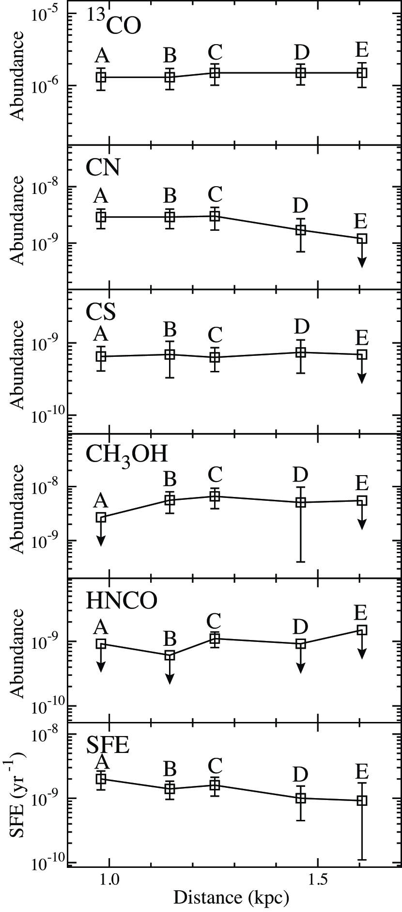
Figure 9: Fractional abundances of CN, CS, CH₃OH, and HNCO relative to H₂ as a function of the galactocentric distance (top five figures). The star formation efficiency (SFE) as a function of the garactocentric distance (bottom figure). Squares with arrow indicate upper limits.

Figure 9 shows the fractional abundances of ¹³CO, CN, CS, CH₃OH, and HNCO relative to H₂, and the star formation efficiencies (SFE) which are derived by dividing the SFR by the H₂ gas mass, at the C¹⁸O peak positions. They are indicated as a function of the galactocentric distance, where the galactocentric distances are estimated by assuming the distance to M51 of 8.4 Mpc, an inclination angle of 22^∘, and a position angle of 173^∘ (Colombo et al., 2014). The fractional abundances of ¹³CO and CS are found to be almost constant over the observed regions along the spiral arm. On the other hand, the fractional abundances of the other molecules and the SFE slightly depends on positions. The fractional abundances of CN and the SFE are higher at Positions A, B, and C than at D and E by factor of 2–1.5. The fractional abundance of CN and the SFE may be correlated with each other along the spiral arm, as the PCA shows a hint of correlation between the integrated intensity map of CN and the SFR distribution. In contrast, the fractional abundance of CH₃OH is lower at Position A than at the other positions. It apparently differs from the trend in the SFE.

4.3 CH₃OH

In this study, we find that CH₃OH has a relatively high fractional abundance ($\sim 6\times 10^{-9}$). In addition, we also recognize that CH₃OH is distributed differently from the other molecules. CH₃OH is thought to be formed on the cold dust mantle through hydrogenation of CO, since the CH₃OH formation in the gas phase is not efficient (Garrod et al., 2007). Some liberation mechanisms are necessary for CH₃OH to be detected in the gas phase. In the Galactic objects, the enhancement of CH₃OH is usually found in hot cores and hot corinos in star-forming regions (e.g. Jørgensen et al., 2005; Bisschop et al., 2007; Bachiller & Pérez Gutiérrez, 1997). Radiative heatings or/and shocks induced by star formation activities such as protostellar outflows are thought to be main desorption mechanisms of CH₃OH. However, the observed CH₃OH abundance is not clearly correlated but slightly anticorrelated with the SFE in the spiral arm of M51. This result is consistent with the result of our previous observation with the IRAM 30 m telescope at a 1 kpc scale (Watanabe et al., 2014). No relevance of the CH₃OH enhancement to star formation activities at a GMC-scale was found in the bar regions of IC 342 and Maffei 2 (Meier & Turner, 2005, 2012), either. Hence, it is most likely that the star formation feedback does not contribute to the gas-phase CH₃OH abundance in M51 at a 300 pc scale.

Meier & Turner (2005, 2012) concluded that the CH₃OH distribution traces large-scale shocks induced by gas orbital resonance in the bar regions. Indeed, other shock tracers such as SiO are found to be enhanced in the bar regions (Usero et al., 2006; Meier & Turner, 2012). Although our observed position of M51 is not the bar region, spiral shocks may occur in the spiral arm (e.g. Fujimoto, 1968; Roberts, 1969; Shu et al., 1972). Such a spiral shock could be responsible for evaporation of CH₃OH. If the spiral shock causes the enhancement of CH₃OH, the non-uniform distribution of the CH₃OH would be originated from variation of shock effects in the spiral arm (i.e. variation of shock strength and/or internal structure of the arm). Another possible mechanism of the CH₃OH liberation is non-thermal desorption such as cosmic-ray induced UV photon, as discussed in Watanabe et al. (2014). The abundance of CH₃OH estimated in this observation is on the same order of that in the cold quiescent core TMC-1 ($\sim 10^{-9}$), where the non-thermal desorption is thought to be responsible for the widely distributed CH₃OH (Soma et al., 2015). Hence, the non-thermal desorption could also explain the observed CH₃OH abundance in the spiral arm of M51.

In addition to the liberation mechanisms, the efficiency of the CH₃OH formation on grain mantle would also affect the CH₃OH distribution in the spiral arm. For dust temperature higher than 30 K, the CH₃OH formation is inefficient on grain mantle, because CO depletion does not occur above 20 K (e.g. Aikawa et al., 2008). Schinnerer et al. (2010) found that the gas kinetic temperature decreases with the galactocentric distance in M51 on the basis of the LVG analysis of their CO observation. In our observation, the CH₃OH abundance is relatively low in Position A. This position is the closest position to the nuclear region of M51, where the temperature may be higher than the other positions.

Above all, the characteristic distribution of CH₃OH would be originated from a combination of evaporation mechanisms and formation mechanisms of CH₃OH. For further understanding of CH₃OH in the spiral arm, sensitive multi-line observations of CH₃OH in other regions including inter-arm regions where the spiral shock does not occur, as well as detailed analyses of kinematics and physical conditions of molecular gas, are necessary. These are left for future studies.

4.4 Other molecules

In this study, we find a hint that the fractional abundance of CN is correlated with the SFE. If so, the CN production may be related to photodissociation of HCN by UV photons from star formation activities or from the nuclear region (e.g. Ginard et al., 2015). In this case, enhancement of other molecules related to the PDR (photodissociation region), such as CCH and CO⁺, could be expected (e.g. Ginard et al., 2015; Fuente et al., 2006; Pety et al., 2005). Sensitive observations of these molecules are thus interesting.

Meier & Turner (2005, 2012) suggested that HNCO comes from grain mantle by the shock evaporation, because the distribution of HNCO is similar to that of CH₃OH in IC 342 and Maffei 2. The fractional abundance of HNCO in M51 is similar to that in IC 342 ($(1-3)\times 10^{-9}$) (Meier & Turner, 2005). The peak position of HNCO almost coincides with that of CH₃OH in M51, and hence, HNCO in our observation may also come from grain mantle. On the other hand, our PCA suggests that the distribution of HNCO is slightly different from those of the other molecules including CH₃OH, although sensitivity of the HNCO observation is not good. Indeed, the HNCO is detected only in one of five positions (C) although the signal-to-noise ratio is 3.2. From observations of the Galactic GMCs, HNCO has been detected with relatively strong intensities in the GMCs near the Galactic center (e.g. Jackson et al., 1984; Armstrong & Barrett, 1985; Cummins et al., 1986). The fractional abundance toward the hot core of Sgr B2(N) is $1.6\times 10^{-7}$ (Marcelino et al., 2010), while that toward the hot core of Orion KL is much lower ($9\times 10^{-9}$) (Zinchenko et al., 2000) than Sgr B2(N). The HNCO abundance is also known to be enhanced in the shocked region L1157 B1 ($(0.4-1.8)\times 10^{-8}$), where HNCO is liberated from grain mantle (Rodríguez-Fernández et al., 2010). On the other hand, the HNCO abundance is as low as $(1-5)\times 10^{-10}$ in cold clouds (Marcelino et al., 2009), where the gas phase production is considered to be dominant. The fractional abundances in M51 is much lower than abundances in Sgr B2(N) and L1157 B1, while it is slightly higher than that in cold clouds. Hence, evaporation of grain mantle seems to contribute to the gas phase abundance of HNCO. Considering poor correlation with the SFR, a galactic shock may play an important role to some extent as in the case of CH₃OH. Since the surface binding energy of HNCO (2850 K) is lower than that of CH₃OH (4930 K) (McElroy et al., 2013), the difference of their distribution may be due to shock strength. It is suggested that HNCO is thought to be unstable under strong UV field (Roberge et al., 1991; Martín et al., 2008), and this may cause the slight difference between CH₃OH and HNCO distribution. Thus, the meaning of the distribution of HNCO is left for future studies.

5 Concluding Remarks

Our interferometric observations of the 6 molecular species toward the spiral arm of M51 at a spatial resolution of 300 pc reveal that the molecular distributions almost look similar to one another and mainly trace the spiral arm structure. A detailed look at the distributions by the PCA and evaluation of the fractional abundances as a function of the galactocentric distance shows a slight chemical differentiation. It should be noted that the CH₃OH distribution is not well correlated to the SFR. Hence, the effect of the star formation and its feedback is not significant in the CH₃OH distribution averaged over the 300 pc scale under a mild star formation activity environment. Similar results are obtained for HNCO and CS. Rather the galactic scale phenomena occurring in the spiral arm, such as the spiral shocks, would be responsible for the slight chemical differentiation.

Appendix A Preprocessing Procedure in the PCA

In order to compare different physical quantities of the integrated intensities of molecules and the star formation rate, the pixel values of a map are normalized and mean-centered as follows:

$$\widetilde{I}_{i\,j}=\frac{I_{i\,j}-\overline{I}_{i}}{\sigma_{i}},$$ (A1)

where $\widetilde{I}_{i\,j}$, $i$, $j$, $I_{i\,j}$, $\overline{I}_{i}$, and $\sigma_{i}$, are a processed pixel value, an index of molecules or star formation rate, an index of the pixel, a pixel value of the original map, a mean pixel value, and an unbiased estimate of variance of the pixel value, respectively. The mean pixel value is given as:

$$\overline{I}_{i}=\frac{1}{n}\sum^{n}_{j=1}I_{i\,j}.$$ (A2)

where $n$ is the number of pixel. The unbiased estimate of variance of the pixel value is denoted as:

$$\sigma^{2}_{i}=\frac{1}{n-1}\sum^{n}_{j=1}(I_{i\,j}-\overline{I}_{i})^{2}.$$ (A3)

Table 1: Summary of observation

Molecule	Transition	Frequency	Sideband	Beam	Vel. Res.	r.m.s.
		(GHz)			(km s-1)	(mK beam-1)
CH3OH	$2_{0}-1_{0}$ A+	96.741375	LSB	$6.9^{\prime\prime}\times 5.5^{\prime\prime},79.9^{\circ}$	10.0	13.9
CS	$J=2-1$	97.980953	LSB	$6.7^{\prime\prime}\times 5.4^{\prime\prime},76.4^{\circ}$	10.0	14.7
C18O	$J=1-0$	109.782173	USB	$6.0^{\prime\prime}\times 4.8^{\prime\prime},79.6^{\circ}$	10.0	15.7
HNCO	$6_{0\,6}-5_{0\,5}$	109.905749	USB	$6.0^{\prime\prime}\times 4.8^{\prime\prime},79.3^{\circ}$	10.0	16.0
13CO	$J=1-0$	110.201354	USB	$6.0^{\prime\prime}\times 4.8^{\prime\prime},77.6^{\circ}$	5.0	21.9
CN	$N=1-0\,J=3/2-1/2$	113.490970	USB	$5.8^{\prime\prime}\times 4.7^{\prime\prime},78.1^{\circ}$	10.0	24.9

Table 2: Integrated intensities in the M51 P1

Molecule	Frequency	Resolution	CARMA	IRAM 30 m
	(GHz)	(arcsec)	(K km s-1)	(K km s-1)
CH3OH	96.741375	25.4	$0.47\pm 0.14$	$0.52\pm 0.05$
CS	97.980953	25.1	$0.49\pm 0.17$	$0.68\pm 0.08$
C18O	109.782173	22.4	$1.53\pm 0.09$	$1.89\pm 0.14$
HNCO	109.905749	22.4	$0.13\pm 0.11$	$0.32\pm 0.10$
13CO	110.201354	22.3	$7.06\pm 0.19$	$7.48\pm 0.16$
CN	113.490970	21.7	$1.21\pm 0.23$	$2.08\pm 0.05$

Table 3: Positions of the C¹⁸O peaks

Position	R. A. (J2000)	Dec. (J2000)
A	13h 29m 50s.3	+47∘ 11′ 40′′.5
B	13h 29m 50s.1	+47∘ 11′ 31′′.4
C	13h 29m 50s.1	+47∘ 11′ 25′′.1
D	13h 29m 50s.8	+47∘ 11′  9′′.7
E	13h 29m 51s.1	+47∘ 11′  3′′.4

Table 4: Line parameters at the C¹⁸O peaks

Position	Molecule	$T$ Peak	$\int Tdv$	$V_{\rm LSR}$	FWHM
		(mK)	(K km s-1)	(km s-1)	(km s-1)
A	13CO	$419\pm 38$	$16.52\pm 0.79$	$480\pm 5$	$40\pm 5$
	C18O	$116\pm 35$	$4.29\pm 0.92$	$480\pm 10$	$40\pm 10$
	CN	$86\pm 31$	$4.15\pm 0.92$
	CH3OH	$<38$	$<1.0$
	HNCO	$<32$	$<0.84$
	CS	$49\pm 12$	$1.70\pm 0.31$	$480\pm 10$	$30\pm 10$
B	13CO	$516\pm 38$	$21.10\pm 0.94$	$485\pm 5$	$40\pm 5$
	C18O	$125\pm 23$	$5.69\pm 0.65$	$480\pm 10$	$50\pm 10$
	CN	$80\pm 29$	$5.44\pm 1.16$
	CH3OH	$61\pm 30$	$2.72\pm 0.80$	$490\pm 10$	$30\pm 10$
	HNCO	$<26$	$<0.74$
	CS	$56\pm 39$	$2.49\pm 1.04$	$480\pm 10$	$50\pm 10$
C	13CO	$644\pm 38$	$21.93\pm 0.93$	$495\pm 5$	$35\pm 5$
	C18O	$156\pm 38$	$5.31\pm 1.07$	$490\pm 10$	$30\pm 10$
	CN	$95\pm 43$	$5.43\pm 1.43$
	CH3OH	$103\pm 31$	$3.02\pm 0.71$	$500\pm 10$	$20\pm 10$
	HNCO	$58\pm 16$	$1.29\pm 0.40$	$500\pm 10$	$20\pm 10$
	CS	$64\pm 13$	$2.08\pm 0.30$	$490\pm 10$	$30\pm 10$
D	13CO	$431\pm 34$	$12.70\pm 0.64$	$510\pm 5$	$25\pm 5$
	C18O	$120\pm 18$	$2.97\pm 0.36$	$510\pm 10$	$20\pm 10$
	CN	$33\pm 31$	$1.72\pm 0.89$
	CH3OH	$62\pm 33$	$1.65\pm 0.74$	$510\pm 10$	$30\pm 10$
	HNCO	$<26$	$<0.58$
	CS	$48\pm 22$	$1.35\pm 0.49$	$510\pm 10$	$30\pm 10$
E	13CO	$290\pm 46$	$8.24\pm 0.76$	$515\pm 5$	$25\pm 5$
	C18O	$72\pm 22$	$1.87\pm 0.44$	$515\pm 10$	$20\pm 10$
	CN	$<39$	$<0.78$
	CH3OH	$<46$	$<0.92$
	HNCO	$<30$	$<0.60$
	CS	$<41$	$<0.83$

Table 5: Column densities at the C¹⁸O peaks

Position	13CO	C18O	CN	CH3OH	HNCO	CS
	$\times 10^{16}$ (cm-2)	$\times 10^{15}$ (cm-2)	$\times 10^{13}$ (cm-2)	$\times 10^{13}$ (cm-2)	$\times 10^{13}$ (cm-2)	$\times 10^{13}$ (cm-2)
A	$1.6\pm 0.3$	$4.3\pm 1.2$	$3.5\pm 1.0$	$<3.3$	$<1.1$	$(0.8\pm 0.2)$
B	$2.1\pm 0.4$	$5.6\pm 1.3$	$4.6\pm 1.3$	$8.9\pm 3.2$	$<1.0$	$(1.1\pm 0.5)$
C	$2.2\pm 0.4$	$5.3\pm 1.5$	$4.5\pm 1.5$	$9.9\pm 3.1$	$1.7\pm 0.6$	$(1.0\pm 0.2)$
D	$1.3\pm 0.3$	$2.9\pm 0.7$	$1.4\pm 0.8$	$5.4\pm 2.7$	$<0.8$	$(0.6\pm 0.3)$
E	$0.8\pm 0.2$	$1.9\pm 0.6$	$<0.7$	$<3.0$	$<0.8$	$<0.4$

Note. — Errors of the column densities are estimated by taking into account the r. m. s. noise and calibration uncertainty (20 %). The column densities are calculated under the LTE approximation with a rotation temperature of 10 K.

Table 6: Fractional abundances relative to H₂ at the C¹⁸O peaks

Position	13CO	CN	CH3OH	HNCO	CS
A	$(1.3\pm 0.4)\times 10^{-6}$	$(2.9\pm 1.1)\times 10^{-9}$	$<2.7\times 10^{-9}$	$<9.2\times 10^{-10}$	$(6.5\pm 2.4)\times 10^{-10}$
B	$(1.3\pm 0.4)\times 10^{-6}$	$(2.9\pm 1.1)\times 10^{-9}$	$(5.6\pm 2.4)\times 10^{-9}$	$<6.1\times 10^{-10}$	$(6.9\pm 3.6)\times 10^{-10}$
C	$(1.5\pm 0.5)\times 10^{-6}$	$(3.0\pm 1.3)\times 10^{-9}$	$(6.6\pm 2.7)\times 10^{-9}$	$(1.1\pm 0.3)\times 10^{-9}$	$(6.3\pm 2.3)\times 10^{-10}$
D	$(1.5\pm 0.5)\times 10^{-6}$	$(1.7\pm 1.0)\times 10^{-9}$	$(6.4\pm 3.6)\times 10^{-9}$	$<9.2\times 10^{-10}$	$(7.4\pm 3.6)\times 10^{-10}$
E	$(1.5\pm 0.6)\times 10^{-6}$	$<1.2\times 10^{-9}$	$<5.5\times 10^{-9}$	$<1.5\times 10^{-9}$	$<6.9\times 10^{-10}$

Note. — Errors of the column densities are estimated by taking into account the r. m. s. noise and calibration uncertainty (20 %).

Table 7: Correlation matrix

Map name	SFR	13CO	C18O	CS	CN	CH3OH	HNCO
SFR	1.0000
13CO	0.4912	1.0000
C18O	0.4301	0.9204	1.0000
CS	0.4870	0.7901	0.7607	1.0000
CN	0.5132	0.7556	0.6990	0.6889	1.0000
CH3OH	0.0435	0.6093	0.5976	0.5817	0.5551	1.0000
HNCO	0.1202	0.3472	0.3919	0.3723	0.3855	0.3545	1.0000

Table 8: Eigenvectors derived in the principal component analysis

Map name	PC1	PC2	PC3	PC4	PC5	PC6	PC7
SFR	0.2674	-0.7293	-0.2900	0.2289	-0.2694	0.4313	-0.0402
13CO	0.4516	-0.0617	0.1707	-0.3364	0.2379	0.1283	0.7596
C18O	0.4407	0.0074	0.1318	-0.5163	0.2661	0.2086	-0.6383
CS	0.4264	-0.0549	0.0753	-0.1477	-0.6293	-0.6247	-0.0377
CN	0.4159	-0.0890	-0.0269	0.5860	0.5525	-0.4010	-0.0942
CH3OH	0.3403	0.4947	0.3786	0.4463	-0.3127	0.4455	-0.0269
HNCO	0.2444	0.4568	-0.8483	-0.0587	-0.0316	0.0668	0.0550
Eigenvalue percentage (%)	61.1	14.7	10.4	5.2	4.2	3.4	1.0

Note. — Eigenvalue percentages indicate the fractions of the total variance treated by each PC component.

References

- Aalto et al. (1999) Aalto, S., Hüttemeister, S., Scoville, N. Z., & Thaddeus, P. 1999, ApJ, 522, 165
- Aikawa et al. (2008) Aikawa, Y., Wakelam, V., Garrod, R. T., & Herbst, E. 2008, ApJ, 674, 984
- Aladro et al. (2011) Aladro, R., Martín, S., Martín-Pintado, J., et al. 2011, A&A, 535, A84
- Aladro et al. (2013) Aladro, R., Viti, S., Bayet, E., et al. 2013, A&A, 549, A39
- Aladro et al. (2015) Aladro, R., Martín, S., Riquelme, D., et al. 2015, A&A, 579, A101
- Armstrong & Barrett (1985) Armstrong, J. T., & Barrett, A. H. 1985, ApJS, 57, 535
- Bachiller & Pérez Gutiérrez (1997) Bachiller, R., & Pérez Gutiérrez, M. 1997, ApJ, 487, L93
- Bisschop et al. (2007) Bisschop, S. E., Jørgensen, J. K., van Dishoeck, E. F., & de Wachter, E. B. M. 2007, A&A, 465, 913
- Calzetti et al. (2007) Calzetti, D., Kennicutt, R. C., Engelbracht, C. W., et al. 2007, ApJ, 666, 870
- Colombo et al. (2014) Colombo, D., Meidt, S. E., Schinnerer, E., et al. 2014, ApJ, 784, 4
- Costagliola et al. (2011) Costagliola, F., Aalto, S., Rodriguez, M. I., et al. 2011, A&A, 528, A30
- Cummins et al. (1986) Cummins, S. E., Linke, R. A., & Thaddeus, P. 1986, ApJS, 60, 819
- Feldmeier et al. (1997) Feldmeier, J. J., Ciardullo, R., & Jacoby, G. H. 1997, ApJ, 479, 231
- Fuente et al. (2006) Fuente, A., García-Burillo, S., Gerin, M., et al. 2006, ApJ, 641, L105
- Fujimoto (1968) Fujimoto, M. 1968, Non-stable Phenomena in Galaxies, 29, 453
- Garrod et al. (2007) Garrod, R. T., Wakelam, V., & Herbst, E. 2007, A&A, 467, 1103
- Ginard et al. (2015) Ginard, D., Fuente, A., García-Burillo, S., et al. 2015, A&A, 578, A49
- Helfer et al. (2003) Helfer, T. T., Thornley, M. D., Regan, M. W., et al. 2003, ApJS, 145, 259
- Hughes et al. (2013) Hughes, A., Meidt, S. E., Schinnerer, E., et al. 2013, ApJ, 779, 44
- Izumi et al. (2013) Izumi, T., Kohno, K., Martín, S., et al. 2013, PASJ, 65, 100
- Jackson et al. (1984) Jackson, J. M., Armstrong, J. T., & Barrett, A. H. 1984, ApJ, 280, 608
- Jørgensen et al. (2005) Jørgensen, J. K., Schöier, F. L., & van Dishoeck, E. F. 2005, A&A, 437, 501
- Kennicutt et al. (2003) Kennicutt, R. C., Jr., Armus, L., Bendo, G., et al. 2003, PASP, 115, 928
- Koda et al. (2009) Koda, J., Scoville, N., Sawada, T., et al. 2009, ApJ, 700, L132
- Kuno et al. (2007) Kuno, N., Sato, N., Nakanishi, H., et al. 2007, PASJ, 59, 117
- Marcelino et al. (2009) Marcelino, N., Cernicharo, J., Tercero, B., & Roueff, E. 2009, ApJ, 690, L27
- Marcelino et al. (2010) Marcelino, N., Brünken, S., Cernicharo, J., et al. 2010, A&A, 516, A105
- Martín et al. (2006) Martín, S., Mauersberger, R., Martín-Pintado, J., Henkel, C., & García-Burillo, S. 2006, ApJS, 164, 450
- Martín et al. (2008) Martín, S., Requena-Torres, M. A., Martín-Pintado, J., & Mauersberger, R. 2008, ApJ, 678, 245
- Martín et al. (2015) Martín, S., Kohno, K., Izumi, T., et al. 2015, A&A, 573, A116
- McElroy et al. (2013) McElroy, D., Walsh, C., Markwick, A. J., et al. 2013, A&A, 550, A36
- Meier & Turner (2005) Meier, D. S., & Turner, J. L. 2005, ApJ, 618, 259
- Meier & Turner (2012) Meier, D. S., & Turner, J. L. 2012, ApJ, 755, 104
- Meier et al. (2015) Meier, D. S., Walter, F., Bolatto, A. D., et al. 2015, ApJ, 801, 63
- Miyamoto et al. (2014) Miyamoto, Y., Nakai, N., & Kuno, N. 2014, PASJ, 66, 36
- Nakai et al. (1994) Nakai, N., Kuno, N., Handa, T., & Sofue, Y. 1994, PASJ, 46, 527
- Nakajima et al. (2011) Nakajima, T., Takano, S., Kohno, K., & Inoue, H. 2011, ApJ, 728, L38
- Nakajima et al. (2015) Nakajima, T., Takano, S., Kohno, K., et al. 2015, PASJ, 67, 8
- Pety et al. (2005) Pety, J., Teyssier, D., Fossé, D., et al. 2005, A&A, 435, 885
- Roberge et al. (1991) Roberge, W. G., Jones, D., Lepp, S., & Dalgarno, A. 1991, ApJS, 77, 287
- Roberts (1969) Roberts, W. W. 1969, ApJ, 158, 123
- Rodríguez-Fernández et al. (2010) Rodríguez-Fernández, N. J., Tafalla, M., Gueth, F., & Bachiller, R. 2010, A&A, 516, A98
- Sakamoto et al. (2014) Sakamoto, K., Aalto, S., Combes, F., Evans, A., & Peck, A. 2014, ApJ, 797, 90
- Schinnerer et al. (2010) Schinnerer, E., Weiß, A., Aalto, S., & Scoville, N. Z. 2010, ApJ, 719, 1588
- Schinnerer et al. (2013) Schinnerer, E., Meidt, S. E., Pety, J., et al. 2013, ApJ, 779, 42
- Schuster et al. (2007) Schuster, K. F., Kramer, C., Hitschfeld, M., García-Burillo, S., & Mookerjea, B. 2007, A&A, 461, 143
- Shu et al. (1972) Shu, F. H., Milione, V., Gebel, W., et al. 1972, ApJ, 173, 557
- Snell et al. (2011) Snell, R. L., Narayanan, G., Yun, M. S., et al. 2011, AJ, 141, 38
- Soma et al. (2015) Soma, T., Sakai, N., Watanabe, Y., & Yamamoto, S. 2015, ApJ, 802, 74
- Suzuki et al. (1992) Suzuki, H., Yamamoto, S., Ohishi, M., et al. 1992, ApJ, 392, 551
- Takano et al. (2014) Takano, S., Nakajima, T., Kohno, K., et al. 2014, PASJ, 66, 75
- Tercero et al. (2010) Tercero, B., Cernicharo, J., Pardo, J. R., & Goicoechea, J. R. 2010, A&A, 517, A96
- Ungerechts et al. (1997) Ungerechts, H., Bergin, E. A., Goldsmith, P. F., et al. 1997, ApJ, 482, 245
- Usero et al. (2006) Usero, A., García-Burillo, S., Martín-Pintado, J., Fuente, A., & Neri, R. 2006, A&A, 448, 457
- Vinkó et al. (2012) Vinkó, J., Takáts, K., Szalai, T., et al. 2012, A&A, 540, A93
- Watanabe et al. (2014) Watanabe, Y., Sakai, N., Sorai, K., & Yamamoto, S. 2014, ApJ, 788, 4
- Watanabe et al. (2015) Watanabe, Y., Sakai, N., López-Sepulcre, A., et al. 2015, ApJ, 809, 162
- Zinchenko et al. (2000) Zinchenko, I., Henkel, C., & Mao, R. Q. 2000, A&A, 361, 1079