Quickest Change Detection with Mismatched Post-Change Models

Abstract

In this paper, we study the quickest change detection with mismatched post-change models. A change point is the time instant at which the distribution of a random process changes. The objective of quickest change detection is to minimize the detection delay of an unknown change point under certain performance constraints, such as average run length (ARL) to false alarm or probability of false alarm (PFA). Most existing change detection procedures assume perfect knowledge of the random process distributions before and after the change point. However, in many practical applications such as anomaly detection, the post-change distribution is often unknown and needs to be estimated with a limited number of samples. In this paper, we study the case that there is a mismatch between the true post-change distribution and the one used during detection. We analytically identify the impacts of mismatched post-change models on two classical detection procedures, the cumulative sum (CUSUM) procedure and the Shiryaev-Roberts (SR) procedure. The impacts of mismatched models are characterized in terms of various finite or asymptotic performance bounds on ARL, PFA, and average detection delay (ADD). It is shown that post-change model mismatch results in an increase in ADD, and the rate of performance degradation depends on the difference between two Kullback-Leibler (KL) divergences, one is between the priori- and post-change distributions, and the other one is between the true and mismatched post-change distributions.

I Introduction

Change detection is the process of identifying the time instants at which the distribution of a random process changes. It has a wide range of applications in various science, engineering, and financial fields, such as intrusion detection, anomaly detection, quality control, financial market analysis, and medical diagnosis, etc.

Change detection methods can be classified into two categories, offline and online change point detections. In offline change detection, the detector estimates the locations of one or more change points based on the observations of the entire random process or time sequence [1]. Offline methods usually need to detect the number of change points before identifying the location of each change point. Online change detection uses sequential analysis to detect whether a change point has happened before the current time by using all currently observed samples [2]-[11]. Online change detection usually needs to make tradeoff among various performance metrics, such as detection delay, probability of false alarm (PFA), and average run length (ARL) to false alarm, etc.

Quickest change detection is an online detection method, and it aims at minimizing the detection delay of a change point under the constraints of an upper bound on PFA or a lower bound on ARL. The change point itself can be modeled as a random variable with prior distributions. If the prior distribution of the change point is known, then Bayesian change detection, such as the well known Shiryaev procedure [2, 3], can be performed. In [4], Tartakovsky and Veeravalli asymptotically characterize the moments of the detection delay of the Shiryaev procedure by letting the PFA goes to zero, and they show that the Shiryaev procedure is asymptotically optimum in the Bayesian setting under some mild conditions. When the prior distribution of the change point is not known, the online change detection can be performed under the minimax criterion, that is, minimizing the expected delay for some worst case change point distribution. One of the most commonly used minimax change detection procedures is the cumulative sum (CUSUM) procedure proposed by Page [5]. The asymptotic behavior of the CUSUM procedure are characterized by Lorden [6] for independently and identically distributed (i.i.d.) samples, and later extended by Lai [7] for non-i.i.d. samples. It is shown that the CUSUM procedure can minimize the worst-worst-case detection delay as the ARL lower bound goes to infinity. Another popular minimax change detection method is the Shiryaev-Roberts (SR) procedure [2, 3, 8]. The asymptotic optimality of the SR procedure are discussed in [9] and [10].

All above mentioned procedures require precise knowledge of the distribution functions before and after the change point. In many practical applications, such as anomaly detection, it is relatively easy to learn and estimate the prior-change distribution, because there is usually a large amount of data available before the change point, e.g., data collected through normal operation conditions. On the other hand, it is usually difficult to obtain an accurate estimate of the post-change distribution, especially for quickest change detection where a decision needs to be made as soon as possible with a limited number of observations from the post-change distribution. In [7], a modified generalized likelihood ratio (GLR) test is developed to take into consideration of some unknown parameters in the post-change distribution, and it is shown that the modified procedure can attain the same asymptotic lower bound of detection delay as the case of known post-change distribution. In [11], a non-parametric quickest detection method that does not require prior knowledge of the distributions is proposed.

In this paper, we study the performance of quickest change detection with mismatched post-change distribution models. That is, there is a mismatch between the true post-change distribution and the one used in the detection procedure, while the detector is assumed to have ideal knowledge of the prior-change distribution. The mismatch can be caused by the limited amount of training data after the change point. Specifically, we study the impacts of mismatched post-detection models on two classical minimax detection procedures, the CUSUM and SR procedures. The performance of CUSUM and SR procedures with mismatched models is characterized by deriving various finite or asymptotic bounds on the PFA, ARL, and average detection delay (ADD). It is shown that the PFA and ARL of the procedures with mismatched post-detection model can attain the same bounds as those with ideal post-detection models. On the other hand, under the same ARL or PFA constraints, post-change model mismatch results in degradation of ADD, and the rate of degradation is determined by the difference between the true and mismatched post-change distributions, which can be measured as the Kullback-Leibler divergence between the two distributions.

II Problem Formulation

Consider two continuous functions $f(x)$ and $g(x)$ where $\lim_{x\to x_{0}}f(x)=\lim_{x\to x_{0}}g(x)=\infty$. We have the following notations.

$$f(x)\underset{x\to x_{0}}{\preceq}g(x)\Longleftrightarrow\lim_{x\to x_{0}}\frac{f(x)}{g(x)}\leq 1$$ (1)

If both $f(x)\underset{x\to x_{0}}{\preceq}g(x)$ and $g(x)\underset{x\to x_{0}}{\preceq}f(x)$, then the two functions are called asymptotically equivalent as $x\to x_{0}$, and it is denoted as

$$f(x)\underset{x\to x_{0}}{\asymp}g(x)\Longleftrightarrow\lim_{x\to x_{0}}\frac{f(x)}{g(x)}=1$$ (2)

II-A System Model

Consider a random process $x_{1},x_{2},\cdots$. Define ${\bf x}^{k:n}=[x_{k},\cdots,x_{n}]$. Let ${\cal F}_{x}^{n}=\sigma({\bf x}^{1:n})$ be the sigma algebra generated by ${\bf x}^{1:n}$.

Assume there is an unknown change point $\theta$, such that the distribution of the random process before the change point differs from that after the change point. Let ${\bf P}_{k}$ and ${\mathbb{E}}_{k}$ denote the probability measure and the corresponding expectation when the change occurs at $\theta=k$. Under ${\bf P}_{k}$, the conditional probability density function (pdf) is $f_{0,n}(x_{n}|{\bf x}^{1:n-1})$ for $n<k$, and it is $f_{1,n}(x_{n}|{\bf x}^{1:n-1})$ for $n\geq k$. With such a notation, ${\bf P}_{\infty}$ and ${\mathbb{E}}_{\infty}$ can be used to represent the probability measure and the corresponding expectation before the change point, that is, the change point happens at $\theta=\infty$.

Assume the change point is random and it follows a prior distribution ${\bf P}(\theta=k)=\pi_{k}$, for $k=1,\cdots,n$. Define the average probability measure ${\bf P}({\cal E})=\sum_{k=1}^{\infty}\pi_{k}{\bf P}_{k}({\cal E})$, and ${\mathbb{E}}$ is the expectation with respect to ${\bf P}$.

Define the likelihood ratio of the samples ${\bf x}^{k:n}$ as

$$\Lambda_{k:n}=\prod_{i=k}^{n}\frac{f_{1,i}(x_{i}|{\bf x}^{1:i-1})}{f_{0,i}(x_{i}|{\bf x}^{1:i-1})}=\prod_{i=k}^{n}\lambda_{i}$$ (3)

where

$$\lambda_{i}=\frac{f_{1,i}(x_{i}|{\bf x}^{1:i-1})}{f_{0,i}(x_{i}|{\bf x}^{1:i-1})}$$ (4)

It is assumed that $\frac{1}{n}\log\Lambda_{k:k+n}$ converges in probability ${\bf P}_{k}$ to a constant, $D_{10}$, as $n\to\infty$. That is,

$$\lim_{n\to\infty}{\bf P}_{k}\left(\left|\frac{1}{n}\log\Lambda_{k:k+n}-D_{10}\right|>\epsilon\right)=0,\forall\epsilon>0.$$ (5)

When the samples are independent, $D_{10}$ is the Kullback-Leibler divergence between the distributions $f_{1,n}$ and $f_{0,n}$.

II-B Detection Procedures

The quickest change detection is performed sequentially by using the observed data sequence. Define a detection procedure $\delta$ as a mapping from the observed sequence ${\cal F}_{x}^{n}$ to a positive integer $k\leq n$

$$\delta:{\cal F}_{x}^{n}\rightarrow\{k:k\leq n\},n=1,2,\cdots$$ (6)

Since $\delta({\bf x}^{1:n})\leq n$, $\delta({\bf x}^{1:n})$ is a stopping time.

Denote the change point detected by $\delta$ as $\tau$, then the PFA associated with method $\delta$ is defined as

$$\text{PFA}(\delta)={\bf P}_{\infty}(\tau<\theta)$$ (7)

The corresponding ARL is defined as

$$\text{ARL}(\delta)={\mathbb{E}}_{\infty}(\tau)$$ (8)

The average detection delay (ADD) associated with the method $\delta$ is defined as

$$\text{ADD}(\delta)={\mathbb{E}}\left[\tau-\theta|\tau\geq\theta\right]=\sum_{k=1}^{\infty}\pi_{k}{\mathbb{E}}_{k}\left[\tau-k|\tau\geq k\right]$$ (9)

We will study the performance of two classical minimax procedures: the CUSUM procedure and the SR procedure.

II-B1 CUSUM procedure

The CUSUM procedure is

$$\delta_{c}(A)=\inf\{n:C_{n}\geq A\}$$ (10)

where

$$C_{n}=\max_{1\leq k\leq n}\Lambda_{k:n}.$$ (11)

We set $\inf\{\emptyset\}=\infty$.

The test statistics $C_{n}$ can be recursively calculated as

$$C_{n+1}=\max(1,C_{n})\lambda_{n+1},~{}~{}~{}n\geq 1$$ (12)

with $C_{0}=0$.

It was shown by Lorden [6] that under the constraint that the ARL is greater than a threshold $\gamma$, as $\gamma\to\infty$, the CUSUM minimzes the “worst-worst-case” detection delay defined as

$$\text{ESADD}(\delta)=\sup_{\theta\geq 0}\left\{\text{ess}\sup{\mathbb{E}}_{\theta}\left((\tau-\theta)^{+}|{\cal F}_{x}^{\theta}\right)\right\}$$ (13)

The result was generalized by Lai [7] to systems with non-i.i.d. samples.

II-B2 SR procedure

The SR procedure is

$$\delta_{s}(A)=\inf\{n:S_{n}\geq A\}$$ (14)

where

$$S_{n}=\sum_{k=1}^{n}\Lambda_{k:n}.$$ (15)

The test statistics $S_{n}$ can be recursively calculated as

$$S_{n+1}=(1+S_{n})\lambda_{n+1},~{}~{}~{}n\geq 1$$ (16)

with $S_{0}=0$.

Under the constraint that the ARL is greater than a threshold $\gamma>1$, it is shown by Pollak and Tartakovsky in [9] that the SR procedure can minimize the following metric

$$\text{RIADD}=\frac{\sum_{k=0}^{\infty}{\mathbb{E}}_{k}(\tau-k)^{+}}{{\mathbb{E}}_{\infty}(\tau)}$$ (17)

The asymptotic ADD of both CUSUM and SR procedures are studied in [4]. It is shown that if the convergence condition in (5) is satisfied, then

$$\text{PFA}(\delta_{c}(A)) \leq\alpha$$ (18)

$$\text{PFA}(\delta_{s}(A)) \leq\alpha$$ (19)

for $A={\bar{\theta}}/\alpha$, where $\bar{\theta}=\sum_{k=1}^{\infty}k\pi_{k}$ is the prior mean of the change point.

In addition, for $A={\bar{\theta}}/\alpha$,

$$\text{ADD}(\delta_{c}(A)) \underset{\alpha\to 0}{\asymp}\frac{|\log\alpha|}{D_{10}}$$ (20)

$$\text{ADD}(\delta_{s}(A)) \underset{\alpha\to 0}{\asymp}\frac{|\log\alpha|}{D_{10}}$$ (21)

II-C Detection Procedures with Mismatched Models

The above detection procedures require the knowledge of the distributions of $x$ before and after the change point. In this paper we will consider the model mismatch case that $f_{0,n}(x)$ is perfectly known, yet there are mismatches for the post-change distribution $f_{1,n}(x)$. Denote ${\tilde{f}}_{1,n}(x)$ as the model used by the detection method, and $f_{1,n}(x)$ as the true model. We will study how the post-change model mismatch will affect the performance of the CUSUM and SR detection procedures.

With the mismatched model ${\tilde{f}}_{1,n}(x)$, define the mismatched likelihood ratio

$${\tilde{\lambda}}_{i}=\frac{{\tilde{f}}_{1,i}(x_{i}|{\bf x}^{1:i-1})}{f_{0,i}(x_{i}|{\bf x}^{1:i-1})},$$ (22)

and

$${\tilde{\Lambda}}_{k:n}=\prod_{i=k}^{n}{\tilde{\lambda}}_{i}.$$ (23)

Let ${\tilde{\bf{\bf P}}}_{k}$ denote the mismatched probability measure such that under ${\tilde{\bf{\bf P}}}_{k}$, the conditional probability density function (pdf) is $f_{0,n}(x_{n}|{\bf x}^{1:n-1})$ for $n<k$, and it is ${\tilde{f}}_{1,n}(x_{n}|{\bf x}^{1:n-1})$ for $n\geq k$.

The corresponding mismatched test statistics for the CUSUM and SR procedures can be written, respectively, as

$${\tilde{C}}_{n} =\max_{1\leq k\leq n}{\tilde{\Lambda}}_{k:n}$$ (24)

$${\tilde{S}}_{n} =\sum_{k=1}^{n}{\tilde{\Lambda}}_{k:n}$$ (25)

The above test statistics can be calculated recursively as

$${\tilde{C}}_{n+1} =\max(1,{\tilde{C}}_{n}){\tilde{\lambda}}_{n+1}$$ (26)

$${\tilde{S}}_{n+1} =(1+{\tilde{S}}_{n}){\tilde{\lambda}}_{n+1}$$ (27)

The CUSUM and SR procedures with mismatched models can be represented, respectively, as

$${\tilde{\delta}}_{c}(A) ={\tilde{\tau}}_{c}=\inf\{n:{\tilde{C}}_{n}\geq A\}$$ (28)

$${\tilde{\delta}}_{s}(A) ={\tilde{\tau}}_{s}=\inf\{n:{\tilde{S}}_{n}\geq A\}$$ (29)

III Impacts of Model Mismatch on ARL and PFA

In this section, we study the impacts of post-change model mismatch of the performance of the CUSUM and SR detection procedures, in terms of the ARL and the PFA.

III-A ARL

The ARLs of the CUSUM and SR procedures with mismatched post-change models are studied in this subsection.

Lemma 1

${\tilde{S}}_{n}-n$ is a martingale under the probability measure ${\bf P}_{\infty}$, and ${\mathbb{E}}_{\infty}({\tilde{S}}_{n}-n)=0$.

Proof:

Under the probability measure ${\bf P}_{\infty}$, we have

$${\mathbb{E}}_{\infty}({\tilde{\Lambda}}_{k:n})=\int\frac{d{\tilde{\bf{\bf P}}}_{k}({\bf x}^{k:n}|{\bf x}^{1:k-1})}{d{\bf P}_{0}({\bf x}^{k:n}|{\bf x}^{1:k-1})}d{\bf P}_{0}({\bf x}^{k:n}|{\bf x}^{1:k-1})=1$$ (30)

For the SR procedure, based on the recursive calculation of ${\tilde{S}}_{n+1}$, we have

$${\mathbb{E}}_{\infty}({\tilde{S}}_{n+1}|{\tilde{S}}_{n})=1+{\tilde{S}}_{n}$$ (31)

Thus ${\tilde{S}}_{n}-n$ is a Martingale.

From the definition of ${\tilde{S}}_{n}$, we have ${\mathbb{E}}_{\infty}({\tilde{S}}_{n})=\sum_{k=1}^{n}{\mathbb{E}}_{\infty}({\tilde{\Lambda}}_{k:n})=n$. ∎

Lemma 2

The ARL for both the CUSUM and SR procedures with mismatched post-change models satisfy

$$\text{ARL}({\tilde{\delta}}_{c}(A)) \geq A$$ (32)

$$\text{ARL}({\tilde{\delta}}_{s}(A)) \geq A$$ (33)

Proof:

If ${\mathbb{E}}_{\infty}({\tilde{\tau}}_{s})=\infty$, then $\text{ARL}({\tilde{\delta}}_{c}(A))=\infty\geq A$.

We will next consider the case when ${\mathbb{E}}_{\infty}({\tilde{\tau}}_{s})<\infty$. From (31), it is straightforward that ${\mathbb{E}}_{\infty}[|{\tilde{S}}_{n+1}-(n+1)-{\tilde{S}}_{n}-n|{\tilde{S}}_{n}]=0$. Based on the optional stopping theorem, we have

$${\mathbb{E}}_{\infty}({\tilde{S}}_{{\tilde{\tau}}_{s}}-{\tilde{\tau}}_{s})={\mathbb{E}}_{\infty}({\tilde{S}}_{1}-1)=0$$ (34)

Thus

$${\mathbb{E}}_{\infty}({\tilde{\tau}}_{s})={\mathbb{E}}_{\infty}({\tilde{S}}_{{\tilde{\tau}}_{s}})\geq A$$ (35)

Since ${\tilde{C}}_{n}\leq{\tilde{S}}_{n}$, under the same threshold $A$, we have ${\tilde{\tau}}_{c}\geq{\tilde{\tau}}_{s}$, thus ${\mathbb{E}}_{\infty}({\tilde{\tau}}_{c})\geq{\mathbb{E}}_{\infty}({\tilde{\tau}}_{s})\geq A$. ∎

III-B PFA

Lemma 3

The PFA of the SR procedure with mismatched model is upper bounded by

$$\text{PFA}({\tilde{\delta}}_{s}(A))\leq\min\left\{\frac{\bar{\theta}}{A},1\right\}$$ (36)

where ${\bar{\theta}}=\sum_{k=1}^{\infty}k\pi_{k}$ is the priori mean of the change point $\theta$.

Proof:

Since ${\tilde{S}}_{n}-n$ is a martingale with respect to ${\bf P}_{\infty}$, ${\tilde{S}}_{n}$ is a sub-martingale with respect to ${\bf P}_{\infty}$. Based on Doob’s inequality, we have

$${\bf P}_{\infty}({\tilde{\tau}}_{s}<n)={\bf P}_{\infty}\left(\max_{1\leq k<n}{\tilde{S}}_{k}\geq A\right)\leq\frac{n}{A}$$ (37)

Therefore

$${\bf P}({\tilde{\tau}}_{s}<\theta)=\sum_{k=1}^{\infty}\pi_{k}{\bf P}_{\infty}({\tilde{\tau}}_{s}<k)=\frac{\bar{\theta}}{A}$$ (38)

∎

Lemma 4

The PFA of the CUSUM procedure with mismatched model is upper bounded by

$$\text{PFA}({\tilde{\delta}}_{c}(A))\leq\frac{1}{A}\leq\frac{\bar{\theta}}{A}$$ (39)

Proof:

It can be easily shown that ${\tilde{C}}_{n}$ is a sub-Martingale because

$${\mathbb{E}}_{\infty}({\tilde{C}}_{n+1}|{\tilde{C}}_{n})=\max(1,{\tilde{C}}_{n})\geq{\tilde{C}}_{n}$$ (40)

In addition, ${\mathbb{E}}_{\infty}({\tilde{C}}_{n})=\max_{1\leq k\leq n}{\mathbb{E}}_{\infty}(\Lambda_{k:n})=1$.

Based on Doob’s inequality, we have

$${\bf P}_{\infty}({\tilde{\tau}}_{c}<n)={\bf P}_{\infty}\left(\max_{1\leq k<n}{\tilde{C}}_{k}\geq A\right)\leq\frac{1}{A}$$ (41)

Therefore

$${\bf P}({\tilde{\tau}}_{c}<\theta)=\sum_{k=1}^{\infty}\pi_{k}{\bf P}_{\infty}({\tilde{\tau}}_{c}<k)=\frac{1}{A}$$ (42)

The second inequality in (39) is from the fact that $\bar{\theta}\geq\min(\theta)=1$. ∎

From the above results, we have

$$\text{PFA}\left(\delta_{c}\left(\frac{1}{\alpha}\right)\right) \leq\alpha$$ (43)

$$\text{PFA}\left(\delta_{s}\left(\frac{\bar{\theta}}{\alpha}\right)\right) \leq\alpha$$ (44)

Based on the above analysis, it can be seen that a mismatch in the post-change distribution have no impact on the ARL lower bound or PFA upper bound, because the ARL and PFA are calculated with respect to the probability measure ${\bf P}_{\infty}$, and they will only be affected by the distribution prior to the change.

IV ADD with Mismatched Models

The ADD of CUSUM and SR procedures with mismatched post-change distributions are studied in this section.

In order to study the impact of model mismatch on ADD, we define the likelihood ratio between the true and mismatched post-change distributions as

$${\tilde{\lambda}}^{11}_{n}=\frac{f_{1}(x_{n}|{\bf x}^{1:n-1})}{{\tilde{f}}_{1}(x_{n}|{\bf x}^{1:n-1})}$$ (45)

and

$${\tilde{\Lambda}}^{11}_{k:n}=\prod_{i=k}^{n}{\tilde{\lambda}}^{11}_{i}$$ (46)

In addition to the convergence assumption in (5), it is assumed that $\frac{1}{n}\log{\tilde{\Lambda}}^{11}_{k:k+n}$ converges in probability ${\bf P}_{k}$ to a constant, ${\tilde{D}}_{11}$ , that is

$$\lim_{n\to\infty}{\bf P}_{k}\left(\left|\frac{1}{n}\log{\tilde{\Lambda}}^{11}_{k:k+n}-{\tilde{D}}_{11}\right|>\epsilon\right)=0,\forall\epsilon>0,$$ (47)

We will study the ADD by considering two cases: $D_{10}-{\tilde{D}}_{11}>0$ or $D_{10}-{\tilde{D}}_{11}<0$.

IV-A $D_{10}-{\tilde{D}}_{11}>0$

We will derive an asymptotic upper bound on ADD as the PFA $\alpha\to 0$. To obtain the upper bound, define a new stopping time

$$\beta(A)=\inf\{n\geq k:{\tilde{\Lambda}}_{k:n}\geq A\}$$ (48)

We have the following lemma regarding the asymptotic behavior of $\beta(A)$ as $A\to\infty$.

Lemma 5

Assume the convergence condition in (5) and (47) are satisified. If ${\tilde{D}}_{11}<D_{10}$, as $A\to\infty$, we have

$${\mathbb{E}}_{k}[(\beta(A)-k)^{+}]\underset{A\to\infty}{\preceq}\frac{\log A}{D_{10}-{\tilde{D}}_{11}},~{}~{}~{}\forall q\neq m$$ (49)

where $a^{+}=a$ if $a\geq 0$ and $a^{+}=0$ otherwise.

Proof:

From (3), (23) and (46), we have

$$\log{\tilde{\Lambda}}_{k:n}=\log\Lambda_{k:n}-\log{\tilde{\Lambda}}_{k:n}^{11}$$ (50)

Based on the convergence condition in (5) and (47), for any $\epsilon>0$, there exists $N_{\epsilon}<\infty$ such that for all $n>N_{\epsilon}$,

$$\left|\frac{\log\Lambda_{k:n}}{n-k+1}-D_{10}\right|<\frac{\epsilon}{2},~{}~{}a.s.$$ (51)

$$\left|\frac{\log{\tilde{\Lambda}}_{k:n}^{11}}{n-k+1}-{\tilde{D}}_{11}\right|<\frac{\epsilon}{2},~{}~{}a.s.$$ (52)

with respect to ${\bf P}_{k}$.

Thus from (50)

$$\left|\frac{\log{\tilde{\Lambda}}_{k:n}}{n-k+1}-(D_{10}-{\tilde{D}}_{11})\right|\leq\\ \left|\frac{\log\Lambda_{k:n}}{n-k+1}-D_{10}\right|+\left|\frac{\log{\tilde{\Lambda}}_{k:n}^{11}}{n-k+1}-{\tilde{D}}_{11}\right|<\epsilon,~{}~{}a.s.$$ (53)

for all $n>N_{\epsilon}$ with respect to ${\bf P}_{k}$.

For any $0<\epsilon<D_{10}-{\tilde{D}}_{11}$, define

$$T_{\epsilon}=\sup\left\{n\geq 1:\left|\frac{\log{\tilde{\Lambda}}_{k:n}}{n-k+1}-(D_{10}-{\tilde{D}}_{11})\right|\geq\epsilon\right\}$$ (54)

Thus $T_{\epsilon}\leq N_{\epsilon}<\infty$.

Based on the definition of $\beta(A)$ in (65), it is obvious that

$${\tilde{\Lambda}}_{k:\beta(A)-1}<A$$ (55)

When $\beta(A)-1>T_{\epsilon}$, we have

$$\frac{\log{\tilde{\Lambda}}_{k:\beta(A)-1}}{\beta(A)-k}-(D_{10}-{\tilde{D}}_{11})>-\epsilon$$ (56)

Thus

$$\beta(A) <k+\frac{\log{\tilde{\Lambda}}_{k:\beta(A)-1}}{D_{10}-{\tilde{D}}_{11}-\epsilon},\text{~{}~{}when~{}~{}}\beta(A)>T_{\epsilon}+1$$

$$\beta(A) \leq T_{\epsilon}+1,\text{~{}~{}when~{}~{}}\beta(A)\leq T_{\epsilon}+1$$

Therefore

$$\beta(A) <k+1+\frac{\log{\tilde{\Lambda}}_{k:\beta(A)-1}}{D_{10}-{\tilde{D}}_{11}-\epsilon}+T_{\epsilon}$$ (57)

$$<k+1+\frac{\log A}{D_{10}-{\tilde{D}}_{11}-\epsilon}+T_{\epsilon}$$ (58)

Since $\epsilon$ can be arbitrarily small and $T_{\epsilon}<\infty$, let $\epsilon\to 0$ we have

$$\lim_{A\to\infty}\frac{{\mathbb{E}}_{k}[\beta(A)-k]}{\frac{\log A}{D_{10}-{\tilde{D}}_{11}}}<1$$ (59)

∎

With the results in Lemma 5, we can obtain an asymptotic upper bound of the ADD with mismatched post-change models, and the results are given in the following theorem.

Theorem 1

Assume the convergence condition in (5) and (47) are satisified. Let $\text{PFA}<\alpha$. If ${\tilde{D}}_{11}<D_{10}$, as $\alpha\to 0$, we have

$${\mathbb{E}}[{\tilde{\tau}}_{c}-\theta|{\tilde{\tau}}_{c}>\theta] \underset{\alpha\to 0}{\preceq}\frac{\frac{|\log\alpha|}{1-\alpha}}{D_{10}-{\tilde{D}}_{11}}$$ (60)

$${\mathbb{E}}[{\tilde{\tau}}_{s}-\theta|{\tilde{\tau}}_{s}>\theta] \underset{\alpha\to 0}{\preceq}\frac{\frac{\log{\bar{\theta}}-\log\alpha}{1-\alpha}}{D_{10}-{\tilde{D}}_{11}}$$ (61)

Proof:

The ADD of the CUSUM procedure with mismatched model can be alternatively written as

$${\mathbb{E}}[{\tilde{\tau}}_{c}-\theta|{\tilde{\tau}}_{c}>\theta]=\frac{1}{{\bf P}_{\infty}({\tilde{\tau}}_{c}\geq\theta)}\sum_{k=1}^{\infty}\pi_{k}{{\mathbb{E}}_{k}({\tilde{\tau}}_{c}-k)^{+}}$$ (62)

By definition, we have ${\tilde{\tau}}_{c}<\beta(A)$, thus from Lemma 5,

$${\mathbb{E}}_{k}({\tilde{\tau}}_{c}-k)^{+}\underset{A\to\infty}{\preceq}\frac{\log A}{D_{10}-{\tilde{D}}_{11}}$$ (63)

From (43), we can set $A=\frac{1}{\alpha}$ to guarantee $\text{PFA}<\alpha$. Thus ${\bf P}_{\infty}({\tilde{\tau}}_{c}\geq\theta)=1-\text{PFA}\geq 1-\alpha$. Combining (62), (63) and the above results, we have

$${\mathbb{E}}[{\tilde{\tau}}_{c}-\theta|{\tilde{\tau}}_{c}>\theta]\underset{\alpha\to 0}{\preceq}\frac{\frac{|\log\alpha|}{1-\alpha}}{D_{10}-{\tilde{D}}_{11}}$$ (64)

For the upper bound of ${\tilde{\tau}}_{s}$, from (44), we can set $A=\frac{\bar{\theta}}{\alpha}$ to ensure $\text{PFA}<\alpha$. The remaining procedures are the same as the analysis of ${\tilde{\tau}}_{c}$. ∎

IV-B $D_{10}-{\tilde{D}}_{11}<0$

To facilitate analysis, define a new stopping time

$$\zeta_{v}(A)=\inf\{n\geq v:{\tilde{\Lambda}}_{v:n}\geq A\}$$ (65)

We have the following lemma regarding the behavior of $\zeta_{v}(A)$ when $D_{10}-{\tilde{D}}_{11}<0$.

Lemma 6

Assume the convergence condition in (5) and (47) are satisified. If $D_{10}-{\tilde{D}}_{11}<0$ and $A>1$, then

$${\mathbb{E}}_{k}[(\zeta_{v}(A)-k)^{+}]=\infty$$ (66)

Proof:

Define $Z_{n}=\log{\tilde{\Lambda}}_{v:n}=Z_{n-1}+\log{\tilde{\lambda}}_{n}$.

1) When $v<k$, we have

$${\mathbb{E}}_{k}(Z_{n+1}|Z_{n})=Z_{n}+(D_{10}-{\tilde{D}}_{11}),\text{~{}for all~{}}n\geq k$$ (67)

Thus $Z_{n}-n(D_{10}-{\tilde{D}}_{11})$ forms a martingale for all $n\geq k$, with ${\mathbb{E}}_{k}(Z_{k})=D_{10}-{\tilde{D}}_{11}$

Proof by contradiction. Assume $E_{k}[\zeta_{v}(A)|\zeta_{v}(A)>k]<\infty$. Then based on optional stopping theorem, we have

$${\mathbb{E}}_{k}[Z_{\zeta_{v}(A)}|\zeta_{v}(A)>k]-{\mathbb{E}}_{k}[\zeta_{v}(A)|\zeta_{v}(A)\geq k](D_{10}-{\tilde{D}}_{11})=$$

$${\mathbb{E}}_{k}[Z_{k}]-k(D_{10}-{\tilde{D}}_{11})=-(k-1)(D_{10}-{\tilde{D}}_{11})$$ (68)

Thus when $A>1$,

$${\mathbb{E}}_{k}[\zeta_{v}(A)-(k-1)|\zeta_{v}(A)\geq k] =-\frac{{\mathbb{E}}_{k}[Z_{\zeta_{v}(A)}]}{|D_{10}-{\tilde{D}}_{11}|}$$ (69)

$$\leq-\frac{\log A}{|D_{10}-{\tilde{D}}_{11}|}<0$$ (70)

This contradicts with ${\mathbb{E}}_{k}[\zeta_{v}(A)-(k-1)|\zeta_{v}(A)\geq k]\geq 0$. Thus ${\mathbb{E}}_{k}[\zeta_{v}(A)|\zeta_{v}(A)\geq k]=\infty$. Since ${\bf P}(\zeta_{v}(A)\geq k)>0$, we have ${\mathbb{E}}_{k}[(\zeta_{v}(A)-k)^{+}]=\infty$.

2) When $v\geq k$, we have

$${\mathbb{E}}_{k}(Z_{n+1}|Z_{n})=Z_{n}+(D_{10}-{\tilde{D}}_{11}),\text{~{}for all~{}}n\geq v$$ (71)

Thus $Z_{n}-n(D_{10}-{\tilde{D}}_{11})$ forms a martingale for all $n\geq v$, with $E_{k}(Z_{v})=D_{10}-{\tilde{D}}_{11}$.

Proof by contradiction. Assume $E_{k}[\zeta_{v}(A)|\zeta_{v}(A)\geq v]<\infty$. Then based on optional stopping theorem, we have

$${\mathbb{E}}_{k}[Z_{\zeta_{v}(A)}|\zeta_{v}(A)\geq v]-{\mathbb{E}}_{k}[\zeta_{v}(A)|\zeta_{v}(A)\geq v](D_{10}-{\tilde{D}}_{11})=$$ (72)

$${\mathbb{E}}_{k}[Z_{v}]-v(D_{10}-{\tilde{D}}_{11})=-(v-1)(D_{10}-{\tilde{D}}_{11})$$ (73)

Thus when $A>1$,

$${\mathbb{E}}_{k}[\zeta_{v}(A)-(v-1)|\zeta_{v}(A)\geq v] =-\frac{{\mathbb{E}}_{k}[Z_{\zeta_{v}(A)}]}{|D_{10}-{\tilde{D}}_{11}|}$$ (74)

$$\leq-\frac{\log A}{|D_{10}-{\tilde{D}}_{11}|}<0$$ (75)

This contradicts with ${\mathbb{E}}_{k}[\zeta_{v}(A)-(v-1)|\zeta_{v}(A)\geq v]\geq 0$. Thus ${\mathbb{E}}_{k}[(\zeta_{v}(A)-v)^{+}]=\infty$. Since $v\geq k$, we have ${\mathbb{E}}_{k}[(\zeta_{v}(A)-k)^{+}]\geq{\mathbb{E}}_{k}[(\zeta_{v}(A)-v)^{+}]=\infty$. ∎

Theorem 2

Assume the convergence condition in (5) and (47) are satisified. Let $\text{PFA}<\alpha<1$. If $D_{10}-{\tilde{D}}_{11}<0$, then the ADD of the CUSUM procedure satisfies

$${\mathbb{E}}[{\tilde{\tau}}_{c}-\theta|{\tilde{\tau}}_{c}\geq\theta]=\infty$$ (76)

Proof:

Based on the definition of ${\tilde{\tau}}_{c}$ and $\zeta_{v}(A)$, we have

$${\tilde{\tau}}_{c}=\min_{v}\zeta_{v}(A)$$ (77)

From (43), we can set $A=\frac{1}{\alpha}$ to ensure $\text{PFA}<\alpha$. Since $\alpha<1$, thus $A>1$. From Lemma 6, we have

$${\mathbb{E}}_{k}({\tilde{\tau}}_{c}-k)^{+}=\min_{v}{\mathbb{E}}(\zeta_{v}(A)-k)^{+}=\infty$$ (78)

Thus

$${\mathbb{E}}[{\tilde{\tau}}_{c}-\theta|{\tilde{\tau}}_{c}\geq\theta]=\frac{1}{{\bf P}({\tilde{\tau}}_{c}\geq\theta)}\sum_{k=1}^{\infty}\pi_{k}{\mathbb{E}}_{k}({\tilde{\tau}}_{c}-k)^{+}=\infty$$ (79)

∎

Please note the infinity ADD result in Theorem 2 is not an asymptotic result and it only requires $\alpha<1$. Such a non-asymptotic result is in general not true for the SR procedure. If the asymptotic condition $\log({\tilde{S}}_{n})\underset{\alpha\to 0}{\asymp}\log({\tilde{C}}_{n})$ is satisfied, then we have ${\mathbb{E}}[{\tilde{\tau}}_{s}-\theta|{\tilde{\tau}}_{s}\geq\theta]\underset{\alpha\to 0}{\rightarrow}\infty$ when $D_{10}-{\tilde{D}}_{11}<0$.

V Numerical Results

Numerical and simulation results are provided in this section to verify the analytical bounds obtained in this paper. In the simulations, all data follow a two-dimension multivariate Gaussian distribution with zero-mean and covariance matrix

$${\bf R}=\left[\begin{array}[]{cc}1&\rho\\ \rho&1\end{array}\right].$$ (82)

The coefficient $\rho$ before and after the change point is 0 and 0.5, respectively. The prior distribution of the change point is the geometric distribution with parameter $p_{0}$, that is, $\pi_{k}=(1-p_{0})^{k-1}p_{0}$. We set $p_{0}=0.1$ in all simulations.

Fig. 1 compares the ADD of CUSUM with true or mismatched post-change point models as a function of the logarithm of the detection threshold. As indicated by Theorem 1, the asymptotic upper bound is linear in $\log A$, with slope inversely proportional to $D_{10}-{\tilde{D}}_{11}$. Under the configuration in this simulation, we have $D_{10}=0.1438$, ${\tilde{D}}_{11}=0.0308$ for $\rho=0.3$, and ${\tilde{D}}_{11}=0.0090$ for $\rho=0.4$. Thus the ADD of the true model has the smallest slope, and the ADD of the mismatched model with $\rho=0.3$ has the largest slope. The ADDs obtained through simulations are also approximately linear in $\log A$, and they follow the same trends as their respective upper bounds.

We compare the ADDs of systems with the CUSUM and SR procedures in Fig. 2. For comparison purpose, we use the same threshold $A$ for both procedures. It can be seen that even the upper bound is pretty tight for the CUSUM procedure, it is loose for the SR procedure. The SR procedure considerably outperforms the CUSUM procedure in terms of ADD, for both true models and mismatched models. The performance gain of SR in terms of ADD is achieved at the cost of PFA and ARL, as will be shown in Figs. 4 and 3. When $\log A>3.5$, we can see that the ADD curves of both CUSUM and SR procedures with mismatched models share the same slope as the upper bound.

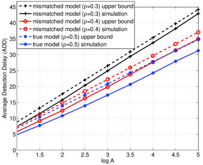
Figure 1: Average detection delay of the CUSUM procedure.

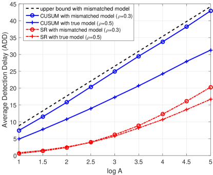
Figure 2: Average detection delay of both CUSUM and SR procedures.

The ARLs obtained with various detection procedures are shown in Fig. 3 as a function of the logrithm of the threshold $A$. For the mismatched model after the change point, the coefficient $\rho$ is assumed to be 0.3, while the true model uses $\rho=0.5$. The mismatched model has very small impact on the ARL to false alarm, for both CUSUM and SR procedures. For the CUSUM procedure, using $\rho=0.3$ instead of its true value 0.5 results in a slight increase in the ARL. For the SR procedure, the ARLs of system with true or mismatched post-change model are almost the same. The SR procedure has a smaller ARL than CUSUM.

Fig. 4 shows the PFA of various detection procedures and their corresponding upper bounds. All parameters are the same as Fig. 3. The CUSUM procedure outperforms the SR procedure in terms of PFA, for both true and mismatched post-change model. It is interesting to note that using a mismatched coefficient of $\rho=0.3$ leads to a smaller PFA than using the true coefficient $\rho=0.5$, for both CUSUM and SR procedures.

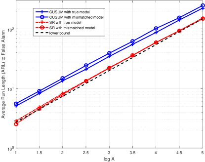
Figure 3: Average run length to false alarm.

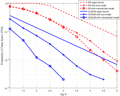
Figure 4: Probability of false alarm.

VI Conclusions

We have studied the quickest change detection when there is a mismatch between the true post-change distribution and the one used by the detection procedures. The performance of two commonly used minimax procedures, the CUSUM procedure and the Shiryaev-Roberts procedure, have been characterized in this paper. The impacts of mismatched post-change model on the ARL, PFL, and ADD have been identified in terms of various finite or asymptotic performance bounds. Detection procedures with mismatched post-change models can attain the same ARL lower bound or PFA upper bound as those with true models. On the other hand, the ADD will be increased significantly due to model mismatch. When $D_{10}-{\tilde{D}}_{11}>0$, the ADD is asymptotically upper bounded. When $D_{10}-{\tilde{D}}_{11}<0$, the ADD of the CUSUM procedure is infinity.

References

• [1] B. Zhang, J. Geng, and L. Lai, β€œMultiple change-points estimation in linear regression models via sparse group Lasso ,” IEEE Trans. Sig. Processing, vol. 63, pp. 2209-2224, 2015.
• [2] A. N. Shiryaev, β€œThe Problem of the most rapid detection of a disturbance in a stationary process,” Soviet Mathematics Doklady, vol. 2, pp. 295-799, 1961.
• [3] A. N. Shiryaev, β€œOn optimum methods in quickest detection problems,” Theory of probability and its applications, vol. 8, pp. 22-46, 1963.
• [4] A. G. Tartakovsky, and V. V. Veeravalli, β€œGeneral asymptotic Bayesian theory of quickest change detection,” Theory Probab. Appl., vol. 49, pp. 458-497, 2005.
• [5] E. S. Page, β€œContinuous inspection schemes,” Biometrika, vol. 41, pp. 100 115, 1954.
• [6] G. Lorden, β€œProcedures for reacting to a change in distribution,” Annals of Mathematical Statistics, vol. 42, pp. 1897 1908, 1971.
• [7] T. L. Lai, β€œInformation bounds and quick detection of parameter changes in stochastic systems,” IEEE Trans. Info. Theory, vol. 44, pp. 2917-2929, Nov. 1998.
• [8] S. W. Roberts, β€œA comparison of some control chart procedures,” Technometrics, vol. 8, pp. 411-430, 1966.
• [9] M. Pollak and A. G. Tartakovsky, β€œOptimality properties of the Shiryaev Roberts procedure,” Statistica Sinica, vol. 19, pp. 1729-1739, 2009.
• [10] A. G. Tartakovsky, and George V. Moustakides, β€œState-of-the-art in Bayesian changepoint detection,” Sequential Analysis, vol. 49, pp. 125-145, 2010.
• [11] T. Banerjee, H. Firouzi, and A. O. Hero, β€œNon-parametric quickest change detection for large scale random matrices,” in Proc. IEEE Intl Symposium on Information Theory ISIT’15, Hong Kong, 2015.