A computational model relating the self-assembly in a fluid of lath like particles with its rheology and gelation

Abstract

We study the self-assembly leading to a gel transition occurring in a numerical model of a solution of slender, colloidal sized particles, called laths, who interact mostly in the direction perpendicular to their areas. At the particle level, the attraction causes them to align into long aggregates of several particles, called whiskers in the literature. To simulate the process, we have developed a Brownian dynamics model in which the attractive interaction comes from a potential energy that depends on both the relative orientation of the laths as well as normal vectors to their areas, disregarding their width. The simplicity of the model allows the simulation to reach large enough times, of the order of minutes, needed to simulate numerical rheology tests. With this we are able to characterize the whisker formation, as well as to simulate the gel transition. A a conclusion of this work, we have shown that the gel transition can occur even if the whiskers are not allowed to branch, as is the case in this model.

1 Introduction

In the present letter, we want to study both the structure and rheology of aggregates of long slender particles using a computational model. This aggregates are called whiskers in the literature. In order to retain just the basic elements of the system, the particles are simulated as a slender plane, a lath, that is defined by just two directions, one along the long axis and one perpendicular to it. The potential energy that generates the stacking depends on only one energetic parameter. It consists on the product of two functions, one that depends on the relative orientation among laths and one that represents an excluded volume contribution. In combination with a Brownian dynamics method, this allows to produce a fast and simple model which generates and allows to study the aggregation of the laths into whiskers. Our lath model deviates from the Brownian dynamics simulations that study the aggregation of rod like particles, as in [8].

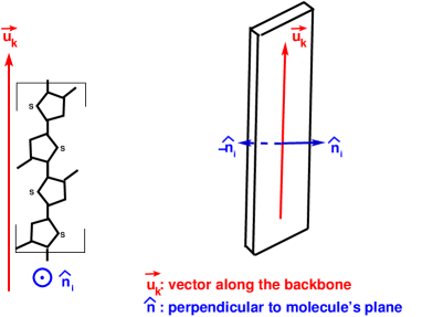
Figure 1: Model of the molecule. The direction $\mathbf{\hat{u}}_{k}$, in red, is defined along the backbone of the P3HT molecule. The normal $\mathbf{\hat{n}}$, in blue, is defined perpendicular to the plane of the molecule. (Left) The backbone is specifically depicted. (Right) In the three dimensional representations there are two $\mathbf{\hat{n}}$ vectors. They are further explained in 4

In order to provide an experimental system, we will make reference to the aggregates of P3HT molecules. For that particular case our model is just a rough estimate, since we will not be taking into account the flexibility of such molecule. Furthermore the whole molecule should be coarse grained into a single lath, which can be seen as a very bold approximation. However, our numerical simulations show a very good resemblance to the rheology of such system, which shows that the highly coarse graining is not far from the physics of this phenomenon.

The strong forces between molecules (or macromolecules) who have a $\pi$ structure is known in the literature as aromatic, or simply $\pi-\pi$ interaction [7]. In the case of some of semi-flexible polymers, it is known to cause stacking of the aromatic groups; which in turn drives a self-assembly process that creates structures orders of magnitude larger than the length of the original particles[14, 1].

An important process that develops $\pi$ stacking is the polymer component used in creation of hetero-junctions of organic solar cells being, for instance, a mixture of P3HT and $C_{60}$ [15, 20]. One particularly interesting problem, both from the simulation and the experimental point of view, is to understand the process of formation of the interface between the two components; as it affects the performance of the capture of the energy by the solar cell [5]. For instance, some experimental groups have studied the relationship between the molecule characteristics with the final behavior of the cell is of special relevance [13].

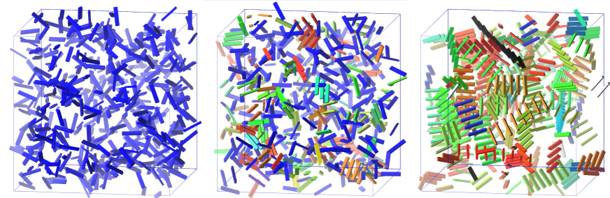
Figure 2: Snapshots of one simulation. T = $40$ $K$, and the rest of the parameters are those of [1]. (Left): Initial state of the simulation. The color code corresponds to different whiskers, with blue being the color of free laths. (Middle): $t=0.5$ $s$, starting to create some whiskers. (Right) : At $t=200$ $s$, several long whiskers. (Color online.)

On the macroscopic level, the self-assembly process generates a change in the rheology: the gelation of the solution [9]. One particularly clever experimental set-up consists in probing this network by comparing measurements of the electrical conductivity and the rheology of such gels [17, 16]. We are able to pursue similar rheological tests with our present computational model. Specifically, we can test the loss and storage modulus of the system while changing the temperature. This provides a way to test the possibility of gelation.

Previous computational studies (Langevin coarse grained and MD simulations) have studied both the self-assembly process of the P3HT molecules into whiskers, [19, 11, 10]; as well as the gel formation [12]. Although successful, these models have the drawback of relying in complex force fields; which are both computationally expensive and difficult to interpret by isolating the individual interactions. To the best of our knowledge, no similar coarse grained simulations of stacking of particles have been attempted, either in polymer or colloidal systems.

2 Model and simulations

We propose the model to be named Brownian Orientational Lath Model, and to use the acronym BOLD.

2.1 Configurations and interactions

As already emphasized above, our goal is to investigate the gel transition of strongly interacting lath-like objects of colloidal sizes. Although the basic system to which we apply our model will be that of $\pi$-stacking polythiophenes in solution, we will keep the model itself as generic as possible. We therefore consider as basic object of our simulations a lath as depicted in 1. We describe its position the three Cartesian coordinates $\mathbf{r}=\left\{x,y,z\right\}$ of its center of mass, and its orientation in space by and the two perpendicular unit vectors $\mathbf{\hat{u}}$ and $\mathbf{\hat{n}}$. Subscripts will indicate the particular lath under consideration. The vector $\mathbf{\hat{u}}$ specifies the direction of the long axis of the lath while $\mathbf{\hat{n}}$ is chosen to be perpendicular to the plane spanned by the two longest edges of the lath. In all that follows it is assumed that the shortest of the three edges is much shorter than the others, as is the case in P3HT.

We propose to describe the potential of a given configuration as

$$\Phi_{S}=\epsilon\sum_{j,k}V_{d}(r_{kj})V_{o}(\mathbf{\hat{u}}_{k},\mathbf{\hat{u}}_{j})V_{cn}(\mathbf{\hat{n}}_{k}\cdot\mathbf{r}_{kj})V_{cn}(\mathbf{\hat{n}}_{j}\cdot\mathbf{r}_{kj}),$$ (1)

where $\mathbf{r}_{kj}=\mathbf{r}_{k}-\mathbf{r}_{j}$, is connector between two laths, and $r_{kj}$ is its length. The first factor in each term describes the dependence of the interaction energy on the distance between the centers of mass of the two laths under consideration, and the three other factors describe the dependence on their relative orientations. The explicit expressions are as follows

$$V_{d}(r_{kj}) = \frac{1}{2}\left(\frac{\tanh\left(a\left(r_{kj}-\frac{\sigma}{2}\right)\right)}{\tanh\left(\frac{a\sigma}{2}\right)}-1+\frac{A_{excl}}{(r-r_{excl})^{4}}\right)$$

$$V_{o}(\mathbf{\hat{u}}_{k},\mathbf{\hat{u}}_{j}) = (\mathbf{\hat{u}}_{k}\cdot\mathbf{\hat{u}}_{j})^{2}$$

$$V_{cn}(\mathbf{\hat{n}}_{k},\mathbf{\hat{r}}_{kj}) = \begin{cases}(\mathbf{\hat{n}}_{k}\cdot\mathbf{\hat{r}}_{kj})^{2}&\mbox{ if }\mathbf{\hat{n}}_{k}\cdot\mathbf{\hat{r}}_{kj}>0\\ 0&\mbox{ else }\end{cases}.$$

The second factor, $V_{o}(\mathbf{\hat{u}}_{k},\mathbf{\hat{u}}_{j})$, favors a parallel orientation for the long axis of the two laths. The last two factors, $V_{cn}(\mathbf{\hat{n}}_{k}\cdot\mathbf{r}_{kj})$ and $V_{cn}(\mathbf{\hat{n}}_{j}\cdot\mathbf{r}_{kj})$, minimize the energy when the two vectors $\mathbf{\hat{n}}_{k}$ and $\mathbf{\hat{n}}_{j}$ are both parallel to the connector $\mathbf{r}_{kj}$, thereby favoring the two faces of the laths to be parallel. The reason for distinguishing between positive and negative values of $\mathbf{\hat{n}}_{j}\cdot\mathbf{r}_{kj}$ will be explained below. Expression $V_{d}(r_{kj})$ is plotted in 3. The minimum is seen to be at a distance between two laths of about $0.4*L_{lath}$. This implies that the thickness of the lath plus the face-to-face distance is about equal to this value. In the simulations, the potential is linearized below a $0.3*L_{lath}$ to allow for acceptable time steps. The values of the various parameters in $V_{d}(r_{kj})$ are given in [1].

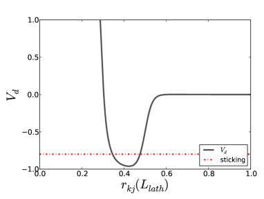
Figure 3: The dependence of the potential with the distance,$V_{d}(r_{k,j})$, is a narrow function with its center close to $0.4$ $L_{lath}$. Below a certain cutoff, $r_{cutoff}=0.3$ $L_{lath}$, it is replaced with a linear extension. The threshold for sticking and unsticking is close to the bottom of the well, that is $0.2\epsilon$ above the absolute bottom of the well, in the dash-dotted red line. (Color online.)

Within a whisker, a lath is strongly bound to one; or, more commonly, to two other laths. In order to complete the description of the potential energy, we must define when this binding within two laths happens. This will be the case when their interaction energy is less than a threshold energy $V_{thr}$ for which we choose $V_{thr}=-0.8\epsilon$. Then, two laths which are strongly bound to each other, while none of the two laths is strongly bound to another lath, interact like a pair of free laths.

2.2 Propagator and refinement of potential

In general there is no qualitative difference between the dynamics of $\mathbf{\hat{u}}_{k}$ and that of $\mathbf{\hat{n}}_{k}$, a simulation shall treat both with the same methods and precision. Notice, however, that $\mathbf{\hat{n}}_{k}$ is by definition perpendicular to $\mathbf{\hat{u}}_{k}$, so that $\mathbf{\hat{u}}_{k}$ has three degrees of freedom and $\mathbf{\hat{n}}_{k}$ has one less. In the case of lath-like particles, rotations around the long axes will be much faster than reorientations of $\mathbf{\hat{u}}_{k}$ or displacements of the laths as a whole; in other words, the dynamics of $\mathbf{\hat{n}}_{k}$ will be much faster than that of $\mathbf{\hat{u}}_{k}$. We will therefore assume that during one time step the lath has fully explored all possible orientations around its long axis and has settled into the corresponding energetic minimum. This means that during the simulation the vector $\mathbf{\hat{n}}_{k}$ will be determined by the configuration described by $\left\{\mathbf{r}_{k},\mathbf{\hat{u}}_{k}\right\}$ and its recent history (see below). We are then left with two equations of motion for each particle:

$$d\mathbf{r}_{k} = -\frac{1}{\xi_{0}}\nabla_{k}\Phi_{C}dt+\nabla_{k}\left(\frac{k_{B}T}{\xi_{0}}\right)dt+\boldsymbol{\Theta}_{k}^{t}\sqrt{\frac{2k_{B}Tdt}{\xi_{0}}}.$$ (2)

$$d\mathbf{\hat{u}}_{k} = \frac{L_{lath}^{2}}{9\xi_{0}}\mathbf{T}\times\mathbf{\hat{u}}_{k}dt+\boldsymbol{\Theta}_{k}^{r}\frac{L_{lath}}{3}\sqrt{\frac{2k_{B}Tdt}{\xi_{0}}}$$ (3)

Here $\boldsymbol{\Theta}_{k}^{t}$ is a three dimensional random vector with components which have zero mean and unit variance, uncorrelated among each other. Similarly $\boldsymbol{\Theta}_{k}^{r}$ is a two dimensional random vector with uncorrelated components having zero mean and unit variance. The two random rotations are applied around two perpendicular axes orthogonal to $\mathbf{\hat{u}}_{k}$. After each time step the length of the vector $\mathbf{\hat{u}}_{k}$ is brought back to unity by a shortening along the original orientation [3, 21]. $\xi_{0}$ is the average translational friction of the lath; we have chosen the rotational friction to be related to the translational friction as for infinitely long rods [4, 21].

Let us now describe how we update $\mathbf{\hat{n}}_{k}$. First, consider two laths $k$ and $j$, neither of whom is interacting with any other lath. We choose $\mathbf{n}_{k}=\mathbf{r}_{kj}-(\mathbf{r}_{kj}\cdot\mathbf{\hat{u}}_{k})\mathbf{\hat{u}}_{k}$, and similarly for $\mathbf{\hat{n}}_{j}$, since these are the orientations assumed to correspond to the minimum interaction between the two laths for the given configuration $\left\{\mathbf{r}_{kj},\mathbf{\hat{u}}_{k},\mathbf{\hat{u}}_{j}\right\}$; unit vector $\mathbf{\hat{n}}_{k}$ is $\mathbf{n}_{k}/\sqrt{\mathbf{n}_{k}\cdot\mathbf{n}_{k}}$. This choice will drive the two laths to become parallel and have their centers of mass connector $\mathbf{r}_{kj}$ perpendicular to both $\mathbf{\hat{u}}_{k}$ and $\mathbf{\hat{u}}_{j}$. Substituting these expressions for $\mathbf{\hat{n}}_{k}$ and $\mathbf{\hat{n}}_{j}$ into the potential above leaves us with a simple pair potential as commonly used in simulations of hard convex bodies.

The situation is different when a free lath $j$ interacts with a lath $k$, which is strongly interacting with another lath $s(k)\neq j$. In this case lath $j$ may still freely reorient along its long axis, but lath $k$ is restricted to do so by its strong interaction with $s(k)\neq j$. We therefore choose $\mathbf{\hat{n}}_{j}$ as above, but set $\mathbf{\hat{n}}_{k}$ equal to the normalized $\mathbf{n}_{k}=\mathbf{r}_{s(k),k}-(\mathbf{r}_{s(k),k}\cdot\mathbf{\hat{u}}_{k})\mathbf{\hat{u}}_{k}$. The $s(k)$ is strongly bound to lath $k$. We are now in the situation where we need to distinguish between two cases in the definition of $V_{cn}$. Only when lath $j$ is situated on the positive side of lath $k$ it may bind to lath $k$; on the negative side lath $k$ is already bound to lath $s(k)$ and cannot bind to the newly arriving lath $j$ anymore. Notice that this treatment of the re-orientations of the laths around their long axes turns the potential in this case into a three body potential. Moreover the potential becomes history dependent. This is similar to coarse grain simulations of linear polymers [18], where the entangling of polymers is not fully determined by the configuration of the beads, but depends on how the beads came to that particular configuration.

A third situation occurs when two laths $k$ and $j$ approach each other, but are already bound to $s(k)\neq j$ and $s(j)\neq k$ respectively. In this case we have $\mathbf{n}_{k}=\mathbf{r}_{s(k),k}-(\mathbf{r}_{s(k),k}\cdot\mathbf{\hat{u}}_{k})\mathbf{\hat{u}}_{k}$ and similarly for $\mathbf{n}_{j}$. Only when lath $j$ is on the positive side of lath $k$, determined by lath $s(k)$, and lath $k$ is on the positive side of lath $j$, determined by $s(j)$, will the interaction be non-zero. This treatment turns the interaction into a four-body interaction. The description given above is summarized in 4.

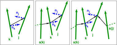
Figure 4: Sketch of the vectors used in the three body potential. The notation is: in bold continuous (green), the orientational vectors $\mathbf{\hat{u}}_{k}$; in thin continuous (black), the connectors; in thick dashed (blue), the normal vector $\mathbf{n}_{k}$; finally in thin dashed (green), possible connectors to other laths. The mathematical model in this letter is three dimensional but, to simplify the sketch, all vectors of this plot lie in the same plane. $s(k)$ is stuck to $k$, and $k$ and $j$ may or may not be stuck together. (left) Neither $k$ nor $j$ is stuck to any other lath (say $l$), then we pick $\mathbf{n}_{k}$ and $\mathbf{n}_{j}$ using the components of the connector that are perpendicular to the respective orientation vectors. (center) $k$ is stuck to $s(k)\neq j$, $j$ does not have another stuck particle; the normal in $k$ is given by its interaction with its stuck particle $s(k)$. (right) Both $k$ and $j$ are stuck to some other laths. (Color online.)

2.3 Parameter settings

A set of nondimensiolanized units are given by the average translational diffusion coefficient of the laths $D_{0}=k_{B}T_{0}/\xi_{0}$, the thermal energy $k_{B}T_{0}$ and the length of a lath $L_{Lath}$. With this choice, the unit of time is $L_{Lath}^{2}/D_{0}$, the unit of velocity is $D_{0}/L_{Lath}$, and the unit of pressure is $k_{B}T/L_{Lath}^{3}$. However, SI units are used in the description of the results of this paper.

All model parameters used in this study are given in [1], once in reduced units and once in SI units. The latter are only used in a few occasions to show that with reasonable parameters the model gives results that are comparable to those found experimentally. The SI parameter settings are meant to be reasonably close to those that apply to P3HT solutions, even though the model that we present here can be used in other contexts. We emphasize that the important characteristics of the model are that bonding can only occur in one-dimensional structures and that the bonding is very strong, $i.e.$ $\epsilon=100k_{B}T_{0}$.

The length of the molecule was chosen to match commercially available P3HT that was reported to us in private communication from an experimental group at TU/e.

Table 1: Parameters used in the model

Parameter	Symbol	Value
Strength of the alignment potential.	$\epsilon$	$4.04\times 10^{-19}J$ $=100k_{B}\times T_{0}$
Length of the laths, unit of distance	$L_{lath}$	$68.44$ $nm$ $\approx 177$ thiophene rings
Length of the size of the squared shaped simulation box	$L_{box}$	$8\times L_{lath}=0.5452$ $\mu m$
Laths in the simulation box	$N_{laths,total}$	$512$
Inflection point of $V_{d}$	$\sigma/2$	$34.22$ $nm$
Cutoff for the linear extension of $V_{d}$	$r_{cutoff}$	$0.3L_{lath}\approx 20.53nm$
Threshold for sticking/unsticking of laths.	$V_{thr.}$	$-0.8\epsilon$
Slope (sharpness) of potential $V_{d}$	$a$	$20m^{-1}$
Excluded volume distance constant	$r_{excluded}$	$0.22L_{lath}\approx 15.05nm$
Excluded volume amplitude	$A_{excluded}$	$0.0001$
Power of the orientational potential	$l$	$1$
Time-step	$\Delta_{t}$	$1\times 10^{-5}s$
Initial Temperature	$T_{0}$	$293$ $K$
Solvent friction (translational)	$\xi_{0}$	$8.66\times 10^{-7}kg/s$
Solvent friction (rotational)	$\xi_{0t}=\frac{\xi_{0}}{9}$	$9.62\times 10^{-8}kg/s$

Results from a typical run with these parameters and at temperature $T=40$ $K$ are shown in 2. In the left panel a box is shown at the beginning of the run. All laths are colored blue indicating that none of them is strongly bound to any of the others. In the middle panel the same box is shown at time $t=50000$, which corresponds to $0.5$ $seconds$ in SI units. It is clearly seen that several laths have collected into short chains, also called whiskers from now on. Laths which are connected through a sequence of consecutive strong bonds are given the same color. Different colors correspond to different whiskers. In the right panel, the same box is shown at $t=20000000$, which corresponds to $200$ $seconds$ in SI units. The box has now reached equilibrium and several long whiskers are observed.

3 Results

In this section we describe the results of our simulations. First we describe the approach to equilibrium of simulations boxes which were initially either fully disordered or fully ordered. This gives information about typical time scales in the system. We also briefly analyze the structure of final equilibrium boxes. In a second subsection we describe the rheological properties of our systems, with special attention being given to the gel transition.

3.1 Time evolution of formation of whiskers and equilibrium distributions of lengths

As we have seen in the previous section, the model parameters chosen in this study lead to the formation of whiskers during simulations starting at time zero with completely disordered boxes. In this section we analyze how this structure evolves with time. To fully characterize the structure of the whiskers we studied several characteristics: its length as a function of time,in number of laths per whisker; the number of whiskers formed in the simulation box, as a function of time; the total material in whiskers as function of time, and the histogram of distribution of whisker sizes.

In 5 we present, for various temperatures, the time evolution of the number of whiskers in our boxes. The left panel corresponds to those that started with randomly distributed laths, while the right hand side panel presents data for boxes starting from fully ordered boxes, i.e. boxes in which all laths were collected in one long whisker. Only the first four or five seconds are shown. The initially ordered simulations serve as a test of the consistency of the model.

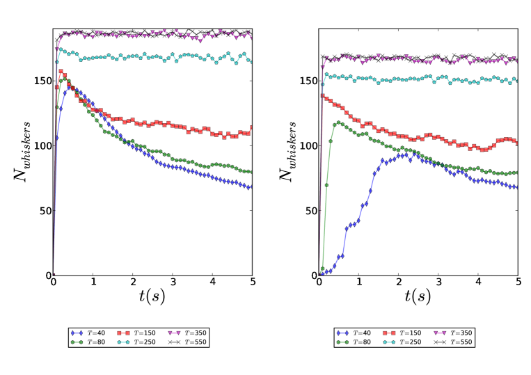
Figure 5: Number of whiskers as function of time, for 6 different temperatures (in Kelvin); first $5$ $s$; average over 20 simulations. (Left) initially disordered configuration, the number of whiskers reaches a higher plateau for higher temperatures. (Right) initially ordered configuration. The only discernible difference between ordered and disordered initial configurations after a few seconds is a lower plateau for the high temperature average number of whiskers in the case of initially ordered simulation. (Color online.)

For temperatures substantially larger than $T_{0}$, large numbers of whiskers (necessarily small) are observed after the first one tenth of a second. In boxes starting from disorder these are obtained by aggregation of laths, while in boxes starting from the ordered structure these are obtained by disintegration of the initially available very long whisker. After the first one tenth of a second hardly any changes occur in the number of whiskers in these boxes. Notice that the various plateau values are not equal for corresponding temperatures in the left and right hand side panels. This is due to the fact that with our code the identification of whiskers is history dependent, as already mentioned in the previous section. This somewhat unrealistic aspect only affects the numbers of very short whiskers.

For temperatures of the order of $T_{0}$ or less, in boxes starting from disorder, again a large number of whiskers is formed within the first few tenths of a second. From then on the number of whiskers start to gradually decrease with increasing time. This is due to the fact that initially only very small whiskers are formed, which then start to merge into longer whiskers. Eventually, equilibrium distributions of lengths occur, depending on the temperature. For these temperatures, boxes starting from ordered configurations behave only slightly differently than those starting from disorder. Again, as in the high temperature case, the long initial whiskers start to disintegrate, but this time increasingly slower with decreasing temperatures. This difference in speed of disintegration is not very important, as we do care most of the equilibrium distribution of initially disordered systems. There are still overshoots in the numbers of whiskers after which the distributions of whiskers begin to rearrange in order to approach the appropriate equilibrium distributions.

In this plot, as well as the ones following, we have included a $T=550$ $K$. The goal of making simulations at this temperature is to show the trend that would have increasing the temperature keeping all the other interactions unchanged. It has to be taken with caution, though, since for a system like P3HT at this temperature one can expect melting to happen.

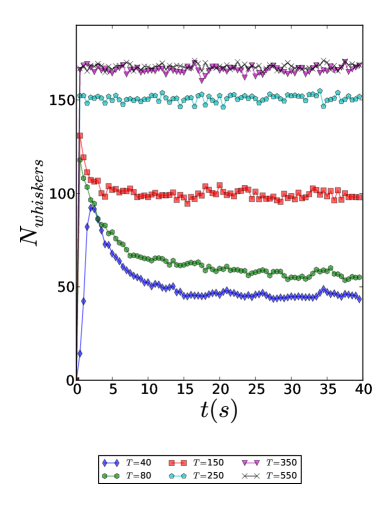
Figure 6: Number of whiskers as function of time, for different temperatures; average over 20 simulations; initially ordered configuration. After the initial sharp growth in number of whiskers there is a decay to a plateau value that depends on the temperature. (Color online.)

In 6 we again present the time evolution of the number of stickers for the same temperatures as above, but this time for a much longer time span of $40$ $s$. Since there is no difference after the first five seconds between the simulations starting from disorder and those starting from order, except for the very high temperatures, we restrict the data here to those of boxes starting from ordered structures. The main conclusion from theses runs is that it is safe to assume that equilibrium distributions have developed only after about twenty to twenty five seconds, depending on temperature.

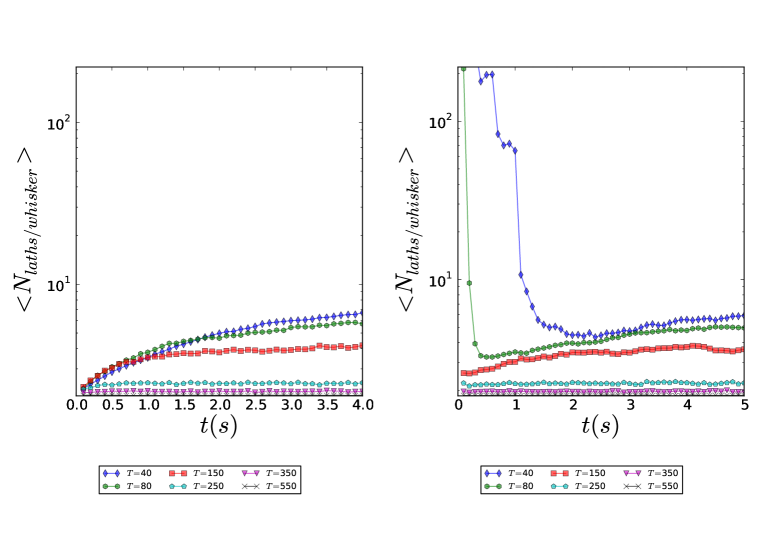
Figure 7: Average number of laths per whisker, as function of temperature; for 20 simulations. In both panels the main axis are set in logarithmic scale.(Left) $4$ $s$ of the initially disordered configuration, (Right) $5$ $s$ of the initially ordered configuration. (Color online.)

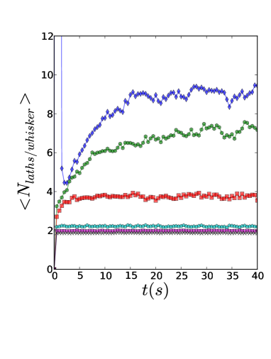
Figure 8: Average number of laths per whisker, as function of temperature; during $40$ $s$; initially ordered configuration; averaged over 20 simulations. Due to a different vertical scale, not all of the data points of 7 are seen here. (Color online.)

7 shows the transient behavior, initial $4$ or $5$ seconds, of the average number of laths per whisker, $<N_{laths/whisker}>$, for both initially disordered and ordered configurations. Notice that the vertical axes are on log scales to more easily span a broad range of values. Both plots show the expected behavior: a steady increase of the number of laths per whisker, for the initially disordered configurations; a breaking up of the initially available whisker spanning the whole box, followed by a steady increase of the number of laths per whisker, for the initially ordered simulations. Again, the lower the temperature, the slower is the time evolution of the towards the final plateau values. 8 shows the long time behavior, up to $40$ $s$, for the initially ordered simulations. As before we notice that up to twenty five seconds are needed before the systems reach equilibrium. Notice also that the high temperature systems reach only average values of two laths per whisker, the minimum value to form a whisker; as the temperature decreases the plateau values grow to values of about ten for the lowest temperature. As temperature increases, longer whiskers are broken into shorter ones, thus reducing the number of laths per whisker.

It is interesting to have a look at the time evolution of the total number of laths taking part in whiskers. These results are shown in 10. Again, in the left panel results refer to systems starting from disorder, while the right panel refers to systems starting from order. It is seen that in systems starting from disorder the total material in whiskers is monotonically increasing, while with systems starting from ordered boxes the total material in whiskers is almost constant; an initial large whisker may split into some whiskers, but does not result into individual laths. It is interesting to notice that after five seconds all simulations have reached their steady state values. This means that after this time the only thing that happens is a rearrangement of the laths in the whiskers in order to approach the appropriate equilibrium distributions. This process takes about twenty seconds. The difference of the total material in whiskers with respect to the temperature comes from the fact that at higher temperatures there is more chance that there are single laths not belonging to any cluster.

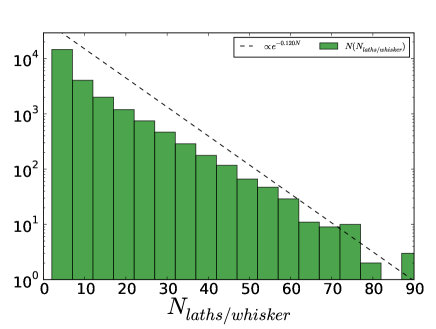
Figure 9: Histogram of laths per whisker; for $10$ different seeds of the random number generator; previously equilibrated by $40$ $s$, and continued by $40$ $s$; at a temperature of $80$ $K$; each simulation having $512$ laths. The line is a function $\propto e^{-0.121N}$, indicating an exponential distribution with $\lambda=1/\overline{N}_{laths/whisker}=1./8.28$, mean $\overline{N}_{laths/whisker}=8.28$. The total number of sampled whiskers for this plot is $23835$.

Next, we are interested in the length-distributions of the whiskers in equilibrium. In 9 we present the distribution of lengths in boxes with temperature $T=80$ $K$. The plot is based on the results of $10$ simulations, starting with different seeds for the random number generators and equilibrated for $40$ $s$, after which production runs of $40$ $s$ each were started. As is clear from the plot, the lengths of whiskers are exponentially distributed, with a mean value of $8.28$ laths per whisker. This results in a slope in 9 of $\lambda=1/8.28\approx 0.121$. The exponential distribution allows for only very few long whiskers; in the present case the longest whiskers found have lengths of about $90$ laths. Nevertheless, such long whiskers quickly deplete the pool of laths, which leads to severe finite size effects for temperatures of about $80$ $K$ or less. This is clearly seen in 11 and 12 where we have plotted the average lengths of whiskers as a function of inverse temperature. The distribution roughly behaves as described in the paper by Cates and Candau on worm-like micelles [2]. In this case the expressions relating the average number of laths per whisker and the temperature are:

$$\ln\left(N_{laths/whisker}-2\right)=\frac{1}{2}\ln\phi+\frac{\epsilon}{2k_{B}T}\ \ \mbox{ for low temperatures }$$

$$\ln\left(N_{laths/whisker}-2\right)=\ln\phi+\frac{\epsilon}{k_{B}T}\ \ \mbox{ for high temperatures }$$ (4)

Our system recovers, quantitatively, the expected trend for low temperatures. The discrepancy with the theory may come from the fact that the boxes have very low number of laths in the simulation box compared to the real system; with only 512 of them, so there may be size effects. This effect is also amplified if we take into the fact that appearance of large whiskers is a rare event.

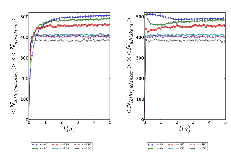
Figure 10: Total material in whiskers (as the product of the average number of whiskers and the average laths per whisker), for different temperatures (in Kelvin); as a function of time and for the first $5$ $s$ of the evolution. (Left) Initially disordered configuration. (Right) Initially ordered configuration. (Color online.)

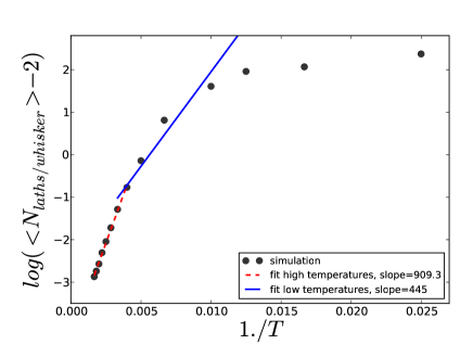
Figure 11: Average number of laths per whisker, against $1/T$. The simulation was run for $40s$ for equilibration and then continued for another $100$ $s$. $T$ in Kelvin. (Color online.)

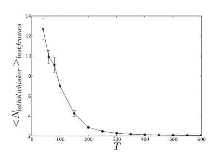
Figure 12: Average number of laths per whisker. The simulation was run for $40s$ for equilibration and then continued for another $100$ $s$. $T$ in Kelvin. The independent variable is $T$.

3.2 Rheology and gel transition

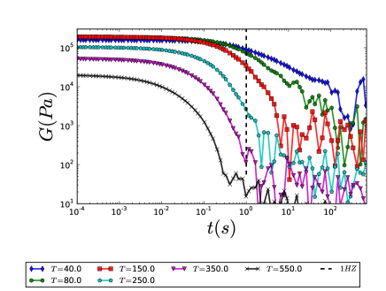
Figure 13: Shear relaxation modulus, $G(t)$, for different values of the temperature of the system. The system equilibrated during (40 $s$); this data was taken after it had run for another 100 $s$. $T$ in Kelvin. (Color online.)

In this section we study the rheological properties of our system. In particular we will investigate how the shear relaxation modulus varies with temperature, and how these variations are related to changes of the distribution of whiskers.

In 13 we present the shear relaxation modulus $G(t)$ as a function of time for various temperatures. Since we are not aiming to study rheological properties like the shear storage and loss moduli, $G^{\prime}$ and $G"$ respectively, in great detail, we did not push calculations of the shear relaxation modulus to convergence for times larger than a few seconds. It is clear from 13 that the plateau value at early times quickly increases with decreasing temperature.

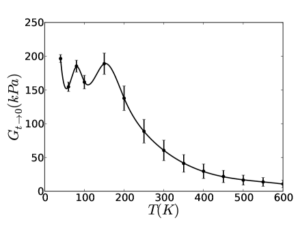
Figure 14: Plateau value for $G$, as function of $T$.

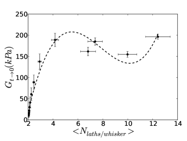
Figure 15: Plateau value for $G$, as function of the number length.

In 14 we present these plateau values as a function of temperature. As is clear from this plot, the zero shear plateau values smoothly increase with decreasing time, up to temperatures of about 200 K. At lower temperatures they fluctuate around an average value of about $170$ kPa. This is probably due to finite size effects as the exponential length distribution becomes severely perturbed since the box can not accommodate sufficiently long whiskers. This has already been noticed above when discussing the average whisker length as function of temperature.

In 15 we plot the same data, but now against the average number of laths per whisker. For small values of $<N_{laths/whisker}>$, $G_{t\rightarrow 0}$ smoothly increases with increasing $<N_{laths/whisker}>$. For large values of the latter, the zero shear plateau fluctuates around a constant value.

Next we recall that the experimental determination of the gel transition is usually based on values of $G^{\prime}$ and $G^{\prime\prime}$ at a frequency of one Hertz. If we now return to the shear relaxation modulus as a function of time (see 13), we notice that at times less than about one second high temperature $G(t)^{\prime}s$ have decayed to very small values, while low temperature $G(t)^{\prime}s$ have not decayed at all. At intermediate temperatures the shear relaxation modulus for $t=1s$ sharply rises. Therefore, in 16 we plot the storage and loss moduli at one Hertz as a function of temperature. It is clear from this plot that for temperatures below about $200K$ the system behaves basically elastic, while for temperatures above $300K$ the system is predominantly viscous. We therefore conclude that according to the usual rheological definition a gel transition occurs at about $250K$. Given the fact that our model has to be taken as highly coarse grained with relation to polymers, we find it remarkable the fact that this behavior is quite similar to that reported in rheological experiments of gelation of P3HT [17]. The main difference of our model with that reference is the absence of hysteresis in our model. It may be caused by the lack of branching of our system, which can be studied in the future.

From the above results we come to the conclusion that the gel transition in whisker forming systems is not a real transition, but depends very much the definition being used. Moreover, being used to different strengths of everyday forces and times will define the gel transition using a different frequency, and arrive at much lower gel transition temperatures.

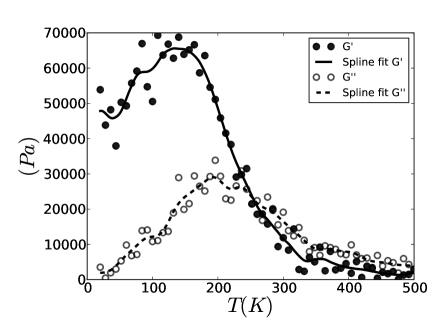
Figure 16: Oscillatory shear numerical experiment. We ran for $60\times 10^{5}$ time steps (60 $s$) discretely increasing the temperature each $1\times 10^{5}$ steps (1 $s$), in 8 $K$ each time. This gives an average rate of 8 $K/s$.

4 Summary

In this letter we have presented a coarse grained model used to study the whisker formation of long slender colloidal sized particles. The model is general, but we argue that it can be also seen as a highly coarse grained model for polymers. In that sense, it can be applied to the aggregation happening due to the $\pi-\pi$ stacking interaction between polythiophenes. For that system, in the crystallized state of the molecule the planes defined by its backbone lie parallel to each other, forming long threads (up to the $\mu m$ scale), called whiskers in the literature. For example, a P3HT molecule of of contour length of 65 nm, produces whiskers of $15\sim 20$ nm width, 5nm thick -two or three chain layers-, and $10\mu m$ long [14]. Here our coarse grained model is a tool to study the rheology, but disregarding the internal flexibility of the molecule (specifically, we do not simulate the hair-pin structure, in which the P3HT bends while crystallizing reaching half of its length. This can be studied in a follow up research).

We propose to model the molecule as a long slender plane, i.e., with a high aspect ratio between the two in-plane directions; which we call a lath. A lath is defined to remain free if the energy of interaction with all its neighbors is above some minimum threshold (small in absolute value or positive). On the contrary a lath within a whisker is stuck to its two closest neighbors and does not interact with the others.

The potential energy depends on a single energetic parameter, and also on the history of the system; having slightly different expressions for two, three and four body interactions. This allows for a very fast algorithm, that can be used to study the rheology of the system. Given our choice of the parameters, we obtain a whisker formation process that reaches an equilibrium state in matter of twenty to twenty five seconds, depending on the temperature. The distribution of number of laths per whisker, which depends on the temperature, has an exponential shape. For $T=80$ $K$, this gives a mean of $8.28$ laths per whisker; similar to the case of worm-like micelles.

Our system, while being simple, does reproduce the gel transition that happens in the case of P3HT in solution. An oscillatory shear experiment that measures $G^{\prime}$ and $G^{\prime\prime}$ while slowly decreasing the temperature $8$ $K$ each $1$ $s$, gives rise to a transition from liquid to gel (imposing a decrease in temperature implies that it is not an strictly closed system, so its entropy does not need to increase). As the transition is the product of the formation of the whiskers, we conclude that part of the rheological changes can be accounted only to the fact of the whisker formation. The gelation process is also seen experimentally, thus we are confident that our model captures the basic physics of the system.

It has been reported in the literature an hysteresis between the ramping up and down of the gelation process [17]. Our system does not show this behavior. A possible reason is the absence of branching in our system. Not having this possibility makes the system pseudo-one dimensional; and since there are no phase transitions for one dimensional structures, while for higher dimensional there are both percolation and phase transitions, it is expected that branching would provide such transitions.

Further improvements to the present model include the study of the interaction between sphere-like particles, like the PCBM or C60, with the laths. It could also be important to study the effect on the alignment that can be obtained by including a second kind of lath, that not necessarily shares the aromatic interaction; as for instance gold nanorods [6].

5 Conclusion

We have investigated the gel transition in $\pi$-stacking long laths, being prototype for moderately long stiff aromatic polymers. The $\pi$-stacking bonds allow for the creation of long whiskers of consecutively stacked laths. We did not allow for branching of such whiskers, thereby preventing the occurrence of extended three-dimensional networks. In particular, the pseudo one-dimensional character of the whiskers does not allow for structural transitions with varying temperatures that could depend on the direction of the temperature gradient; in other words, hysteresis is not present in the gel-sol transition. This character also forces their length distribution to be exponential. As a result, only very few long whiskers occur amidst a see of many smaller whiskers. Chances of having mechanically percolating structures are therefore very low. Nevertheless, we have found that with the usual definition of gel transition, occurring at a temperature where the ratio of the storage and loss moduli at a frequency of one Hertz changes from values larger than one to values lower than one, such a transition indeed does occur. Our main conclusion therefore is that the occurrence of a gel transition does not necessarily imply that percolating three dimensional structures have developed in the system.

6 Acknowledgments

Some of the simulations for this paper used computational time from the “Centro de Informatica y Biología Computacional BIOS”, and ran through the “Red Nacional Académica de Tecnología Avanzada, RENATA”. This work was partially funded by Ozofab, EOST-10023-OZOFAB; and ESMI, Grant Agreement No. 262348 “ESMI”. I want to thank current and former members of the Computational Biophysics Group, specially to Professor Wim Briels, whose dedication, insight and hard work improved the quality of this paper; Professor Wouter den Otter for deep, imaginative and very fruitful discussions; and to Igor Santos de Oliveira, for sharing his knowledge on computational rheology.

7 Bibliography

8 Appendix. Forces and Torques

8.1 Forces

The force acting on lath $i$ is:

$$\mathbf{F}=-\frac{\partial\Phi_{S}}{\partial\mathbf{R}_{i}}.$$

As the potential is the product of different functions is useful to go over their derivatives with respect to $R_{i}$. Take first $V_{d}$:

$$-\frac{\partial V_{d}(r_{kj})}{\partial\mathbf{R}_{i}}=\frac{\epsilon}{2}\left(\frac{-a}{\cosh^{2}(a(r_{kj}-\frac{\sigma}{2}))\tanh\left(\frac{a\sigma}{2}\right)}\right.$$

$$\left.\times\frac{\mathbf{r}_{jk}}{|\mathbf{r}_{jk}|}(\delta_{ik}-\delta_{ij})\right).$$ (5)

The $V_{cn}$ potential takes two forms, depending on the $\mathbf{\hat{n}}_{k}$ vector, either :

$$(\mathbf{\hat{n}}_{k,j,k}\cdot\mathbf{\hat{r}}_{k,j})^{2l},$$ (6)

or

$$(\mathbf{\hat{n}}_{s(k),k,k}\cdot\mathbf{\hat{r}}_{k,j})^{2l}.$$ (7)

One way to calculate the stress components during the simulation, taking into account the periodic boundary conditions, requires to explicitly write the forces as derivatives with respect to the relative vectors $\mathbf{r}_{kj}$ and $\mathbf{r}_{s(k),k}$. As (6) depends on $\mathbf{r}_{kj}$ (there is no $s(k)$ lath to take into account here), then the derivative with respect to either $k$ or $j$ is:

$$-\frac{\partial}{\partial\mathbf{R}_{i}}\left(\frac{\mathbf{n}_{k,j,k}\cdot\mathbf{r}_{k,j}}{|\mathbf{n}_{k,j,k}||\mathbf{r}_{k,j}|}\right)^{2l} = \left[\frac{4l(\mathbf{n}_{k,j,k}\cdot\mathbf{r}_{k,j})^{2l-1}}{(|\mathbf{n}_{k,j,k}||\mathbf{r}_{k,j}|)^{2l}}\mathbf{n}_{k,j,k}\right.$$ (8)

$$- \left.\frac{2l(\mathbf{n}_{k,j,k}\cdot\mathbf{r}_{k,j})^{2l}}{(|\mathbf{n}_{k,j,k}||\mathbf{r}_{k,j}|)^{2l+1}}\left(|\mathbf{r}_{k,j}|\mathbf{\hat{n}}_{k,j,k}+|\mathbf{n}_{k,j,k}|\mathbf{\hat{r}}_{k,j}\right)\right](\delta_{i,k}-\delta_{i,j}).$$

In the case that the potential is (7), the derivative with respect to the coordinates of lath $k$ is:

$$\frac{\partial}{\partial\mathbf{R}_{i}}\left(\frac{\mathbf{n}_{s(k),k,k}\cdot\mathbf{r}_{k,j}}{|\mathbf{n}_{k,j,k}||\mathbf{r}_{k,j}|}\right)^{2l}=\frac{\partial}{\partial\mathbf{r}_{kj}}\left(\frac{\mathbf{n}_{s(k),k,k}\cdot\mathbf{r}_{k,j}}{|\mathbf{n}_{k,j,k}||\mathbf{r}_{k,j}|}\right)^{2l}\frac{\partial\mathbf{r}_{kj}}{\partial\mathbf{R}_{k}}+\frac{\partial}{\partial\mathbf{r}_{k}}\left(\frac{\mathbf{n}_{s(k),k,k}\cdot\mathbf{r}_{k,j}}{|\mathbf{n}_{k,j,k}||\mathbf{r}_{k,j}|}\right)^{2l}\frac{\partial\mathbf{r}_{s(k),k}}{\partial\mathbf{R}_{k}},$$ (9)

Obtaining:

$$\frac{\partial}{\partial\mathbf{r}_{kj}}\left(\frac{\mathbf{n}_{s(k),k,k}\cdot\mathbf{r}_{k,j}}{|n_{k,j,k}||r_{k,j}|}\right)^{2l} = \frac{2l[\mathbf{n}_{s(k),k,k}\cdot\mathbf{r}_{k,j}]^{2l-1}}{[|\mathbf{r}_{k,j}||\mathbf{n}_{s(k),k,k}|]^{2l}}\mathbf{n}_{s(k),k,k}-\frac{2l[\mathbf{n}_{s(k),k,k}\cdot\mathbf{r}_{kj}]^{2l}}{[|\mathbf{r}_{k,j}||\mathbf{n}_{s(k),k,k}|]^{2l+1}}|\mathbf{n}_{s(k),k,k}|\mathbf{\hat{r}}_{k,j}$$

$$\frac{\partial}{\partial\mathbf{r}_{s(k),k}}\left(\frac{\mathbf{n}_{s(k),k,k}\cdot\mathbf{r}_{k,j}}{|n_{k,j,k}||r_{k,j}|}\right)^{2l} = \frac{2l[\mathbf{n}_{s(k),k,k}\cdot\mathbf{r}_{k,j}]^{2l-1}}{[|\mathbf{r}_{k,j}||\mathbf{n}_{s(k),k,k}|]^{2l}}\mathbf{n}_{k,j,k}-\frac{2l[\mathbf{n}_{s(k),k,k}\cdot\mathbf{r}_{kj}]^{2l}}{[|\mathbf{r}_{k,j}||\mathbf{n}_{s(k),k,k}|]^{2l+1}}|\mathbf{r}_{k,j}|\mathbf{\hat{n}}_{s(k),k,k},$$

and :$\frac{\partial\mathbf{r}_{s(k),k}}{\partial\mathbf{R}_{k}}=1$, $\frac{\partial\mathbf{r}_{kj}}{\partial\mathbf{R}_{k}}=-1$. The derivative with respect to $j$,$k$ or $s(k)$ is:

$$-\frac{\partial}{\partial\mathbf{R}_{i}}\left(\frac{\mathbf{n}_{s(k),k,k}\cdot\mathbf{r}_{k,j}}{|n_{k,j,k}||r_{k,j}|}\right)^{2l} = \frac{2l[\mathbf{n}_{s(k),k,k}\cdot\mathbf{r}_{k,j}]^{2l-1}}{[|\mathbf{r}_{k,j}||\mathbf{n}_{s(k),k,k}|]^{2l}}\left(\mathbf{n}_{j,k,k}(\delta_{i,k}-\delta_{i,s(k)})+\mathbf{n}_{s(k),k,k}(\delta_{i,k}-\delta_{i,j})\right)$$

$$+ \frac{2l[\mathbf{n}_{s(k),k,k}\cdot\mathbf{r}_{kj}]^{2l}}{[|\mathbf{r}_{k,j}||\mathbf{n}_{s(k),k,k}|]^{2l+1}}\left(|\mathbf{r}_{k,j}|\mathbf{\hat{n}}_{s(k),k,k}(\delta_{i,k}-\delta_{i,s(k)})-|\mathbf{n}_{s(k),k,k}|\mathbf{\hat{r}}_{k,j}(\delta_{i,k}-\delta_{i,j})\right),$$

8.2 Torques

The definition of the torque is:

$$\mathbf{T}_{i,stk.} = -\mathbf{\hat{u}}_{i}\times\frac{\partial\Phi_{S}}{\partial\mathbf{\hat{u}}_{i}}.$$

And given the torque, the evolution of the orientation vector is given by:

$$d\mathbf{\hat{u}}=\underbrace{[\hat{I}-\mathbf{\hat{u}}\mathbf{\hat{u}}]\cdot\Gamma\cdot\mathbf{\hat{u}}dt}_{\delta u_{i_{1}}}+\underbrace{\frac{1}{\gamma}\mathbf{T}\times\mathbf{\hat{u}}dt}_{\delta u_{i_{2}}}$$ (13)

With $\delta_{u_{1}}$ related to the flow. Both $V_{o}$ and $V_{cn}$ depend on the orientation $\mathbf{\hat{u}}$.

$$-\left(\mathbf{\hat{u}}_{i}\times\frac{\partial V_{so}(\mathbf{r}_{k,j},\mathbf{r}_{s(k),k})}{\partial\mathbf{\hat{u}}_{i}}\right)\times\mathbf{\hat{u}}_{i} = 2l\delta_{i,k}\left(\frac{[\mathbf{n}_{s(k),k,k}\cdot\mathbf{r}_{kj}]^{2l-1}}{[|\mathbf{n}_{s(k),k,k}||\mathbf{r}_{k,j}|]^{2l}}\left(\mathbf{n}_{s(k),k,k}(\mathbf{r}_{k,j}\cdot\mathbf{\hat{u}}_{k})+\mathbf{n}_{k,j,k}(\mathbf{\hat{u}}_{k}\cdot\mathbf{r}_{s(k),k})\right)\right.$$ (14)

$$- \left.\frac{[\mathbf{n}_{s(k),k,k}\cdot\mathbf{r}_{kj}]^{2l}}{|\mathbf{n}_{s(k),k,k}|^{2l+2}|\mathbf{r}_{k,j}|^{2l}}\mathbf{n}_{s(k),k,k}(\mathbf{r}_{s(k),k}\cdot\mathbf{\hat{u}}_{k})\right)$$

For the case in which the orientation vector $\mathbf{n}_{k}$ is not given by a stuck lath the potential is $V_{cn}(\mathbf{\hat{n}}_{k,j,k}\cdot\mathbf{\hat{r}}_{k,j})$, and the analogous calculation gives:

$$- \left(\mathbf{\hat{u}}_{i}\times\frac{\partial V_{so}(\mathbf{r}_{k,j},\mathbf{r}_{s(k),k})}{\partial\mathbf{\hat{u}}_{i}}\right)\times\mathbf{\hat{u}}_{i}=$$

$$2l \delta_{i,k}\left(\frac{(\mathbf{n}_{k,j,k}\cdot\mathbf{r}_{k,j})^{2l-1}}{[|\mathbf{n}_{k,j,k}||\mathbf{r}_{k,j}|]^{2l}}2\mathbf{n}_{k,j,k}(\mathbf{r}_{k,j}\cdot\mathbf{\hat{u}}_{k})-\frac{(\mathbf{n}_{k,j,k}\cdot\mathbf{r}_{k,j})^{2l}}{|\mathbf{n}_{k,j,k}|^{2l+2}|\mathbf{r}_{k,j}|^{2l}}\mathbf{n}_{k,j,k}(\mathbf{r}_{k,j}\cdot\mathbf{\hat{u}}_{k})\right)$$

References

- [1] Martin Brinkmann. Structure and morphology control in thin films of regioregular poly(3-hexylthiophene). Journal of Polymer Science Part B: Polymer Physics, 49(17):1218–1233, 2011.
- [2] M E Cates and S J Candau. Statics and dynamics of worm-like surfactant micelles. Journal of Physics: Condensed Matter, 2(33):6869, 1990.
- [3] Philip D. Cobb and Jason E. Butler. Simulations of concentrated suspensions of rigid fibers: Relationship between short-time diffusivities and the long-time rotational diffusion. The Journal of Chemical Physics, 123(5):054908, 2005.
- [4] M. Doi and S. F. Edwards. The Theory of Polymers Dynamics. Oxford Science Publications, Oxford, U. K., 1986.
- [5] Alain Geiser, Bin Fan, Hadjar Benmansour, Fernando Castro, Jakob Heier, Beat Keller, Karl Emanuel Mayerhofer, Frank Nüesch, and Roland Hany. Poly(3-hexylthiophene)/c60 heterojunction solar cells: Implication of morphology on performance and ambipolar charge collection. Solar Energy Materials and Solar Cells, 92(4):464 – 473, 2008.
- [6] Michael J. A. Hore and Russell J. Composto. Functional polymer nanocomposites enhanced by nanorods. Macromolecules, 47(3):875–887, 2014.
- [7] Christopher A. Hunter and Jeremy K. M. Sanders. The nature of .pi.-.pi. interactions. Journal of the American Chemical Society, 112(14):5525–5534, 1990.
- [8] Navid Kazem, Carmel Majidi, and Craig E. Maloney. Gelation and mechanical response of patchy rods. Soft Matter, 11:7877–7887, 2015.
- [9] Markus Koppe, Christoph J. Brabec, Sabrina Heiml, Alois Schausberger, Warren Duffy, Martin Heeney, and Iain McCulloch. Influence of molecular weight distribution on the gelation of p3ht and its impact on the photovoltaic performance. Macromolecules, 42(13):4661–4666, 2009.
- [10] Cheng K. Lee, Chi C. Hua, and Show A. Chen. Multiscale simulation for conducting conjugated polymers from solution to the quenching state. The Journal of Physical Chemistry B, 113(49):15937–15948, 2009. PMID: 19954241.
- [11] Cheng K Lee, Chi C Hua, and Show A Chen. An ellipsoid-chain model for conjugated polymer solutions. The Journal of Chemical Physics, 136:084901, 2012.
- [12] Cheng K. Lee, Chi C. Hua, and Show A. Chen. Phase transition and gels in conjugated polymer solutions. Macromolecules, 46(5):1932–1938, 2013.
- [13] Sijun Li, Sisi Wang, Baohua Zhang, Feng Ye, Haowei Tang, Zhaobin Chen, and Xiaoniu Yang. Synergism of molecular weight, crystallization and morphology of poly(3-butylthiophene) for photovoltaic applications. Organic Electronics, 15(2):414 – 427, 2014.
- [14] Jung Ah Lim, Feng Liu, Sunzida Ferdous, Murugappan Muthukumar, and Alejandro L. Briseno. Polymer semiconductor crystals. Materials Today, 13(5):14 – 24, 2010.
- [15] Jenny Nelson. Polymer:fullerene bulk heterojunction solar cells. Materials Today, 14(10):462 – 470, 2011.
- [16] Gregory M. Newbloom, Felix S. Kim, Samson A. Jenekhe, and Danilo C. Pozzo. Mesoscale morphology and charge transport in colloidal networks of poly(3-hexylthiophene). Macromolecules, 44(10):3801–3809, 2011.
- [17] Gregory M. Newbloom, Katie M. Weigandt, and Danilo C. Pozzo. Electrical, mechanical, and structural characterization of self-assembly in poly(3-hexylthiophene) organogel networks. Macromolecules, 45(8):3452–3462, 2012.
- [18] J T Padding and W J Briels. Systematic coarse-graining of the dynamics of entangled polymer melts: the road from chemistry to rheology. Journal of Physics: Condensed Matter, 23(23):233101, 2011.
- [19] Kyra N. Schwarz, Tak W. Kee, and David M. Huang. Coarse-grained simulations of the solution-phase self-assembly of poly(3-hexylthiophene) nanostructures. Nanoscale, 5:2017–2027, 2013.
- [20] H. Sirringhaus, P.J. Brown, R.H. Friend, M.M. Nielsen, K. Bechgaard, Langeveld, A.J.H. Spiering, R.A.J. Janssen, E.W. Meijer, P. Herwig, and D.M. de Leeuw. Two-dimensional charge transport in self-organized, high-mobility conjugated polymers. Nature, 401(6754):685–688, 1999.
- [21] Yu-Guo Tao. Kayaking and wagging of rigid rod-like colloids in shear flow. PhD thesis, University of Twente, Enschede, May 2006.
Index