On Distributionally Robust Extreme Value Analysis

Abstract.

We study distributional robustness in the context of Extreme Value Theory (EVT). We provide a data-driven method for estimating extreme quantiles in a manner that is robust against incorrect model assumptions underlying the application of the standard Extremal Types Theorem. Typical studies in distributional robustness involve computing worst case estimates over a model uncertainty region expressed in terms of the Kullback-Leibler discrepancy. We go beyond standard distributional robustness in that we investigate different forms of discrepancies, and prove rigorous results which are helpful for understanding the role of a putative model uncertainty region in the context of extreme quantile estimation. Finally, we illustrate our data-driven method in various settings, including examples showing how standard EVT can significantly underestimate quantiles of interest.

Keywords. Distributional robustness and Generalized extreme value distributions and KL-divergence and Rényi divergence and Quantile estimation

1. Introduction

Extreme Value Theory (EVT) provides reasonable statistical principles which can be used to extrapolate tail distributions, and, consequently, estimate extreme quantiles. However, as with any form for extrapolation, extreme value analysis rests on assumptions that are rather difficult (or impossible) to verify. Therefore, it makes sense to provide a mechanism to robustify the inference obtained via EVT.

The goal of this paper is to study non-parametric distributional robustness (i.e. finding the worst case distribution within some discrepancy of a natural baseline model) in the context of EVT. We ultimately provide a data-driven method for estimating extreme quantiles in a manner that is robust against possibly incorrect model assumptions. Our objective here is different from standard statistical robustness which is concerned with data contamination only (not model error); see, for example, [23], for this type of analysis in the setting of EVT.

Our focus in this paper is closer in spirit to distributionally robust optimization as in, for instance, [8, 14, 3, 4]. However, in contrast to the literature on robust optimization, the emphasis here is on understanding the implications of distributional uncertainty regions in the context of EVT. As far as we know this is the first paper that studies distributional robustness in the context of EVT.

We now describe the content of the paper, following the logic which motivates the use of EVT.

1.1. Motivation and Standard Approach

In order to provide a more detailed description of the content of this paper, its motivations, the specific contributions, and the methods involved, let us invoke a couple of typical examples which motivate the use of extreme value theory. As a first example, consider the problem of forecasting the necessary strength that is required for a skyscraper in New York City to withstand a wind speed that gets exceeded only about once in 1000 years, using wind speed data that is observed only over the last 200 years. In another instance, given the losses observed during the last few decades, a reinsurance firm may want to compute, as required by Solvency II standard, a capital requirement that is needed to withstand all but about one loss in 200 years.

These tasks, and many others in practice, present a common challenge of extrapolating tail distributions over regions involving unobserved evidence from available observations. There are many reasonable ways of doing these types of extrapolations. One might take advantage of physical principles and additional information, if available, in the windspeed setting; or use economic principles in the reinsurance setting. In the absence of any fundamental principles which inform tail extrapolation of a random variable $X,$ one may opt to use purely statistical considerations.

One such statistical approach entails the application of the popular extremal types theorem (see Section 2) to model the distribution of block maxima of a modestly large number of samples of $X,$ by a generalized extreme value (GEV) distribution. Once we have a satisfactory model for the distribution of $M_{n}=\max\{X_{1},\ldots,X_{n}\},$ evaluation of any desired quantile of $X$ is straighforward because of the relationship that $P(M_{n}\leq x)=(P(X\leq x))^{n}$ for any $x\in\mathbb{R}.$ Another common approach is to use samples that exceed a certain threshold to model conditional distribution of $X$ exceeding the threshold. The standard texts in extreme value theory (see, for example, [16, 7, 22]) provide a comprehensive account of such standard statistical approaches.

Regardless of the technique used, various assumptions underlying an application of a result similar to the extremal types theorem might be subject to model error. Consequently, it has been widely accepted that tail risk measures, particularly for high confidence levels, can only be estimated with considerable statistical as well as model uncertainty (see, for example, [15]). The following remark due to [5] holds significance in this discussion: “Though the GEV model is supported by mathematical argument, its use in extrapolation is based on unverifiable assumptions, and measures of uncertainty on return levels should properly be regarded as lower bounds that could be much greater if uncertainty due to model correctness were taken into account.”

Despite these difficulties, however, EVT is widely used (see, for example, [7]) and regarded as a reasonable way of extrapolation to estimate extreme quantiles.

1.2. Proposed Approach Based on Infinite Dimensional Optimization

We share the point of view that EVT is a reasonable approach, so we propose a procedure that builds on the use of EVT to provide upper bounds which attempts to address the types of errors discussed in the remark above from [5]. For large values of $n$, under the assumptions of EVT, the distribution of $M_{n}$ lies close to, and appears like, a GEV distribution. Therefore, instead of considering only the GEV distribution as a candidate model, we propose a non-parametric approach. In particular, we consider a family of probability models, all of which lie in a “neighborhood” of a GEV model, and compute a conservative worst-case estimate of Value atrisk (VaR) over all of these candidate models. For $p\in[0,1],$ the value at risk $\textnormal{VaR}_{p}(X)$ is defined as

$$\textnormal{VaR}_{p}(X)=F^{\leftarrow}(p):=\inf\{x:P\{X\leq x\}\geq p\}.$$

Mathematically, given a reference model, $P_{{}_{\mathnormal{ref}}}$, which we consider to be obtained using EVT (using a procedure such as the one outlined in the previous subsection), we consider the optimization problem

(1) $$\sup\bigg{\{}P\{X>x\}:\ d(P,P_{{}_{\mathnormal{ref}}})\leq\delta\bigg{\}}.$$

Note that the previous problem proposes optimizing over all probability measures that are within a tolerance level $\delta$ (in terms of a suitable discrepancy measure $d$) from the chosen baseline reference model $P_{{}_{\mathnormal{ref}}}.$

There is a wealth of literature that pursues this line of thought (see [8, 14, 1, 3, 4, 12]), but, no study has been carried out in the context of EVT. Moreover, while the solvability of problems as in (1) have understandably received a great deal of attention, the qualitative differences that arise by using various choices of discrepancy measures, $d$, has not been explored, and this is an important contribution of this paper. For tractability reasons, the usual choice for discrepancy $d$ in the literature has been KL-divergence. In Section 3 we study the solution to infinite dimensional optimization problems such as (1) for a large class of discrepancies that includes KL-divergence as a special case, and discuss how such problems can be solved at no significant computational cost.

1.3. Choosing Discrepancy and Consistency Results

One of our main contributions in this paper is to systematically demonstrate the qualitative differences that arise by using different choices of discrepancy measures $d$ in (1). Since our interest in the paper is limited to robust tail modeling via EVT, this narrow scope, in turn, let us analyse the qualitative differences that may arise because of different choices of $d$.

As mentioned earlier, the KL-divergence is the most popular choice for $d$. In Section 4 we show that for any divergence neighborhood $\mathcal{P}$, defined using $d=$ KL-divergence around a baseline reference $P_{{}_{\mathnormal{ref}}}$, there exists a probability measure $P$ in $\mathcal{P}$ that has tails as heavy as

$$P(x,\infty)\geq c\log^{-2}P_{{}_{\mathnormal{ref}}}(x,\infty),$$

for a suitable constant $c$, and all large enough $x.$ This means, irrespective of how small $\delta$ is (smaller $\delta$ corresponds to smaller neighborhood $\mathcal{P}$), a KL-divergence neighborhood around a commonly used distribution (such as exponential, (or) Weibull (or) Pareto) typically contains tail distributions that have infinite mean or variance, and whose tail probabilities decay at an unrealistically slow rate (even logarithmically slow, like $\log^{-2}x$, in the case of reference models that behave like a power-law or Pareto distribution). As a result, computations such as worst-case expected short-fall may turn out to be infinite. Such worst-case analyses are neither useful nor interesting.

For our purposes, we also consider Renyi divergence measures $D_{\alpha}$ (see Section 3.1) that includes KL-divergence as a special case (when $\alpha=1$). It turns out that for any $\alpha>1$, the divergence neighborhoods defined as in $\{P:D_{\alpha}(P,P_{{}_{\mathnormal{ref}}})\leq\delta\}$ consists of tails that are heavier than $P_{{}_{\mathnormal{ref}}}$, but not prohibitively heavy. More importantly, we prove a “consistency” result in the sense that if the baseline reference model belongs to the maximum domain of attraction of a GEV distribution with shape parameter $\gamma_{{}_{\mathnormal{ref}}},$ then the corresponding worst-case tail distribution,

(2) $$\bar{F}_{\alpha,\delta}(x):=\sup\{P(x,\infty):D_{\alpha}(P,P_{{}_{\mathnormal{ref}}})\leq\delta\},$$

belongs to the maximum domain of attraction of a GEV distribution with shape parameter $\gamma^{\ast}=(1-\alpha^{-1})^{-1}\gamma_{{}_{\mathnormal{ref}}}$ (if it exists).

Since our robustification approach is built resting on EVT principles, we see this consistency result as desirable. If a modeler who is familiar with certain type of data expects the EVT inference to result in an estimated shape parameter which is positive, then the robustification procedure should preserve this qualitative property. An analysis of the maximum domain of attraction of the distribution $\bar{F}_{\alpha}(x)$, depending on $\alpha$ and $\gamma_{{}_{\mathnormal{ref}}},$ is presented in Section 4, along with a summary of the results in Table 1.

Note that the smaller the value of $\alpha$, the larger the absolute value of shape parameter $\gamma^{\ast}$, and consecutively, heavier the corresponding worst-case tail is. This indicates a gradation in the rate of decay of worst-case tail probabilities as parameter $\alpha$ decreases to 1, with the case $\alpha=1$ (corresponding to KL-divergence) representing the extreme heavy-tailed behaviour. This gradation, as we shall see, offers a great deal of flexibility in modeling by letting us incorporate domain knowledge (or) expert opinions on the tail behaviour. If a modeler is suspicious about the EVT inference he/she could opt to select $\alpha=1$, but, as we have mentioned earlier, this selection may result in pessimistic estimates.

The relevance of these results shall become more evident as we introduce the required terminology in the forthcoming sections. Meanwhile, Table 1 offers illustrative comparisons of $\bar{F}_{\alpha}(x)$ for various choices of $\alpha.$

1.4. The Final Estimation Procedure

The framework outlined in the previous subsections yields a data driven procedure for estimating VaR which is presented in Section 5. A summary of the overall procedure is given in Algorithm 2. The procedure is applied to various data sets, resulting in different reference models, and we emphasize the choice of different discrepancy measures via the parameter $\alpha$. The numerical studies expose the salient points discussed in the previous subsections and rigorously studied via our theorems. For instance, Example 3 shows how the use of the KL divergence might lead to rather pessimistic estimates. Moreover, Example 4 illustrates how the direct application of EVT can severely underestimate the quantile of interest, while the procedure that we advocate provides correct coverage for the extreme quantile of interest.

The very last section of the paper, Section 6, contains technical proofs of various results invoked in the development.

2. Generalized extreme value distributions

The objective of this section is to mainly fix notation and review properties of generalized extreme value (GEV) distributions that are relevant for introducing and proving our main results in Section 4. For a thorough introduction to GEV distributions and their applications to modeling extreme quantiles, we refer the readers to the wealth of literature that is available (see, for example, [16, 9, 7, 22] and references therein).

If we use $M_{n}$ to denote the maxima of $n$ independent copies of a random variable $X$ with cumulative distribution funtion $F(\cdot),$ then extremal types theorem identifies all non-degenerate distributions $G(\cdot)$ that may occur in the limiting relationship,

(3) $$\lim_{n\rightarrow\infty}P\left\{\frac{M_{n}-b_{n}}{a_{n}}\leq x\right\}=\lim_{n\rightarrow\infty}F^{n}\left(a_{n}x+b_{n}\right)=G(x),$$

for every continuity point $x$ of $G(\cdot),$ with $a_{n}$ and $b_{n}$ representing suitable scaling constants. All such distributions $G(x)$ that occur in the right-hand side of (3) are called extreme value distributions.

Extremal types theorem (Fisher and Tippet (1928), Gnedenko (1943)). The class of extreme value distributions is $G_{\gamma}(ax+b)$ with $a>0,b,\gamma\in\mathbb{R},$ and

(4) $$G_{\gamma}(x):=\exp\left(-\left(1+\gamma x\right)^{-1/\gamma}\right),\quad\quad 1+\gamma x>0.$$

If $\gamma=0,$ the right-hand side is interpreted as $\exp(-\exp(-x)).$

The extremal types theorem asserts that any $G(x)$ that occurs in the right-hand side of (3) must be of the form $G_{\gamma}(ax+b).$ As a convention, any probability distribution $F(x)$ that gives rise to the limiting distribution $G(x)=G_{\gamma}(ax+b)$ in (3) is said to belong to the maximum domain of attraction of $G_{\gamma}(x).$ In short, it is written as $F\in\mathcal{D}(G_{\gamma}).$ The parameters $\gamma,a>0$ and $b$ are, respectively, called the shape, scale and location parameters. From the above we have

$$P(M_{n}\leq x)=P\Big{(}\frac{M_{n}-b_{n}}{a_{n}}\leq\frac{x-b_{n}}{a_{n}}\Big{)}\approx G_{\gamma_{0}}\Big{(}\frac{x-b_{n}}{a_{n}}\Big{)}=:G_{\gamma_{0}}(a_{0}x+b_{0}),$$

where $\gamma_{0},a_{n},b_{n}$ are estimated by a parameter estimation technique such as maximum likelihood and $a_{0}:=1/a_{n}$, $b_{0}:=-b_{n}/a_{n}$. We will use $P_{GEV}$ to denote the distribution $G_{\gamma_{0}}(a_{0}x+b_{0})$.

2.1. Frechet, Gumbel and Weibull types

Though the limiting distributions $G_{\gamma}(ax+b)$ seem to constitute a simple parametric family, they include a wide-range of tail behaviours in their maximum domains of attraction, as discussed below: For a distribution $F,$ let $\bar{F}(x)=1-F(x)$ denote the corresponding tail probabilities, and $x_{{}_{F}}^{*}=\sup\{x:F(x)<1\}$ denote the right endpoint of its support.

• The Frechet Case $(\gamma>0).$ A distribution $F\in\mathcal{D}(G_{\gamma})$ for some $\gamma>0,$ if and only if right endpoint $x_{{}_{F}}^{*}$ is unbounded, and its tail probabilities satisfy

  (5) $$\bar{F}(x)=\frac{L(x)}{x^{1/\gamma}},\quad\quad x>0$$

  for a function $L(\cdot)$ slowly varying at $\infty$. As a consequence, moments greater than or equal to $1/\gamma$ do not exist. Any distribution $F(x)$ that lies in $\mathcal{D}(G_{\gamma})$ for some $\gamma>0$ is also said to belong to the maximum domain of attraction of a Frechet distribution with parameter $1/\gamma.$ The Pareto distribution $1-F(x)=x^{-\alpha}\wedge 1$ is an example for a distribution that belongs to $\mathcal{D}(G_{1/\alpha}).$

• The Weibull case $(\gamma<0).$ Unlike the Frechet case, a distribution $F\in\mathcal{D}(G_{\gamma})$ for some $\gamma<0,$ if and only if its right endpoint $x_{{}_{F}}^{*}$ is finite, and its tail probabilities satisfy

  (6) $$\bar{F}(x_{{}_{F}}^{*}-\epsilon)=\epsilon^{-1/\gamma}L\left(\frac{1}{\epsilon}\right),\quad\quad\epsilon>0$$

  for a function $L(\cdot)$ slowly varying at $\infty.$ A distribution that belongs to $\mathcal{D}(G_{\gamma})$ for some $\gamma<0$ is also said to belong to the maximum domain of attraction of Weibull family. The uniform distribution on the interval $[0,1]$ is an example that belongs to this class of extreme value distributions.

• The Gumbel case $(\gamma=0).$ A distribution $F\in\mathcal{D}(G_{0})$ if and only if

  (7) $$\lim_{t\uparrow x_{{}_{F}}^{*}}\frac{\bar{F}(t+xf(t))}{\bar{F}(t)}=\exp(-x),\quad\quad x\in\mathbb{R}$$

  for a suitable positive function $f(\cdot).$ In general, the members of $G_{0}$ have exponentially decaying tails, and consequently, all moments exist. Probability distributions $F(\cdot)$ that give rise to limiting distributions $G_{0}(ax+b)$ are also said to belong to the Gumbel domain of attraction. Common examples that belong to the Gumbel domain of attraction include exponential and normal distributions.

Given a distribution function $F,$ Proposition 1 is useful to test to determine its domain of attraction:

Proposition 1.

Suppose $F^{\prime\prime}(x)$ exists and $F^{\prime}(x)$ is positive for all $x$ in some left neighborhood of $x_{{}_{F}}^{*}.$ If

(8) $$\lim_{x\uparrow x_{{}_{F}}^{*}}\left(\frac{1-F}{F^{\prime}}\right)^{\prime}(x)=\gamma,$$

then $F$ belongs to the domain of attraction of $G_{\gamma}.$

The proof of Proposition 1 and further details on the classification of extreme value distributions can be found in any standard text on extreme value theory (see, for example, [16] or [7]).

2.2. On model errors and robustness

After identifying a suitable GEV model $P_{{}_{\mathnormal{GEV}}}$ for the distribution of block maxima $M_{n}$, it is common to utilize the relationship $P\{M_{n}\leq x\}=P\{X\leq x\}^{n},$ to compute a desired extreme quantile of $X.$ It is useful to remember that $P_{{}_{\mathnormal{GEV}}}(-\infty,x]$ is only an approximation for $P\{M_{n}\leq x\},$ and the quality of the approximation is, in turn, dependent on the unknown distribution function $F$ (see [22, 7]). Therefore, in practice, one does not know the block-size $n$ for which the GEV model $P_{{}_{\mathnormal{GEV}}}$ well-approximates the distribution of $M_{n}.$ Even if a good choice of $n$ is known, one cannot often employ it in practice, because larger $n$ means smaller $m$, the number of blocks, and consequentially, the inferential errors could be large. Due to the arbitrariness in the estimation procedures and the nature of applications (calculating wind speeds for building sky-scrapers, building dykes for preventing floods, etc.), it is desirable to have, in addition, a data-driven procedure that yields a conservative upper bound for $x_{p}$ that is robust against model errors. To accomplish this, one can form a collection of competing probability models $\mathcal{P},$ all of which appear plausible as the distribution of $M_{n}$, and compute the maximum of $p^{n}$-th quantile over all the plausible models in $\mathcal{P}.$ This is indeed the objective of the sections that follow.

3. A non-parametric framework for addressing model errors

Let $(\Omega,\mathcal{F})$ be a measurable space and $M_{1}(\mathcal{F})$ denote the set of probability measures on $(\Omega,\mathcal{F}).$ Let us assume that a reference probability model $P_{{}_{\mathnormal{ref}}}\in M_{1}(\mathcal{F})$ is inferred by suitable modelling and estimation procedures from historical data. Naturally, this model is not the same as the distribution from which the data has been generated, and is expected only to be close to the data generating distribution. In the context of Section 2, the model $P_{{}_{\mathnormal{ref}}}$ corresponds to $P_{{}_{\mathnormal{GEV}}},$ and the data generating model corresponds to the true distribution of $M_{n}.$ With slight perturbations in data, we would, in turn, be working with a slightly different reference model. Therefore, it has been of recent interest to consider a family of probability models $\mathcal{P},$ all of which are plausible, and perform computations over all the models in that family. Following the rich literature of robust optimization, where it is common to describe the set of plausible models using distance measures (see [3]), we consider the set of plausible models to be of the form

$$\mathcal{P}=\left\{P\in M_{1}(\mathcal{F}):d\left(P,P_{{}_{\mathnormal{ref}}}\right)\leq\delta\right\}$$

for some distance functional $d:M_{1}(\mathcal{F})\times M_{1}(\mathcal{F})\rightarrow\mathbb{R}_{+}\cup\{+\infty\},$ and a suitable $\delta>0.$ Since $d(P_{{}_{\mathnormal{ref}}},P_{{}_{\mathnormal{ref}}})=0$ for any reasonable distance functional, $P_{{}_{\mathnormal{ref}}}$ lies in $\mathcal{P}.$ Therefore, for any random variable $X,$ along with the conventional computation of $E_{{}_{P_{{}_{\mathnormal{ref}}}}}[X],$ one aims to provide “robust” bounds,

$$\inf_{P\in\mathcal{P}}E_{{}_{P}}[X]\leq E_{{}_{P_{{}_{\mathnormal{ref}}}}}[X]\leq\sup_{P\in\mathcal{P}}E_{{}_{P}}[X].$$

Here, we follow the notation that $E_{{}_{P}}[X]=\int XdP$ for any $P\in M_{1}(\mathcal{F}).$ Since the state-space $\Omega$ is uncountable, evaluation of the above $\sup$ and $\inf$-bounds, in general, are infinite-dimensional problems. However, as it has been shown in the recent works [4, 12], it is indeed possible to evaluate these robust bounds for carefully chosen distance functionals $d.$

3.1. Divergence measures

Consider two probability measures $P$ and $Q$ on $(\Omega,\mathcal{F})$ such that $P$ is absolutely continuous with respect to $Q.$ The Radon-Nikodym derivative $dP/dQ$ is then well-defined. The Kullback-Liebler divergence (or KL-divergence) of $P$ from $Q$ is defined as

(9) $$D_{1}(P,Q):=E_{{}_{Q}}\left[\frac{dP}{dQ}\log\left(\frac{dP}{dQ}\right)\right].$$

This quantity, also referred to as relative entropy (or) information divergence, arises in various contexts in probability theory. For our purposes, it will be useful to consider a general class of divergence measures that includes KL-divergence as a special case. For any $\alpha>1,$ the Rényi divergence of degree $\alpha$ is defined as:

(10) $$D_{\alpha}(P,Q):=\frac{1}{\alpha-1}\log E_{{}_{Q}}\left[\left(\frac{dP}{dQ}\right)^{\alpha}\right].$$

It is easy to verify that for every $\alpha,$ $D_{\alpha}(P,Q)=0,$ if and only if $P=Q.$ Additionally, the map $\alpha\mapsto D_{\alpha}$ is nondecreasing, and continuous from the left. Letting $\alpha\rightarrow 1$ in (10) yields the formula for KL-divergence $D_{1}(P,Q).$ Thus KL-divergence is a special case of the family of Rényi divergences, when the parameter $\alpha$ equals $1.$ If the probability measure $P$ is not absolutely continuous with respect to $Q,$ then $D_{\alpha}(P,Q)$ is taken as $\infty.$ Though none of these divergence measures form a metric on the space of probability measures, they have been used in a variety of scientific disciplines to discriminate between probability measures. For more details on the divergences $D_{\alpha},$ see [21, 17].

3.2. Robust bounds via maximization of convex integral functionals

Recall that $P_{{}_{\mathnormal{ref}}}$ is the reference probability measure obtained via standard estimation procedures. Since the model $P_{{}_{\mathnormal{ref}}}$ could be misspecified, we consider all models that are not far from $P_{{}_{\mathnormal{ref}}}$ in the sense quantified by divergence $D_{\alpha},$ for any fixed $\alpha\geq 1.$ Given a random variable $X,$ we consider optimization problems of form

(11) $$V_{\alpha}(\delta):=\sup\left\{E_{{}_{P}}[X]:D_{\alpha}(P,P_{{}_{\mathnormal{ref}}})\leq\delta\right\}.$$

Though KL-divergence has been a popular choice in defining sets of plausible probability measures as above, use of divergences $D_{\alpha},\ \alpha\neq 1$ is not new altogether: see [2, 12]. Due to the Radon-Nikodym theorem, $V_{\alpha}(\delta)$ can be alternatively written as,

(12) $$V_{\alpha}(\delta)=\sup\left\{E_{{}_{P_{{}_{\mathnormal{ref}}}}}[LX]:E_{{}_{P_{{}_{\mathnormal{ref}}}}}[\phi_{\alpha}(L)]\leq\bar{\delta},E_{{}_{P_{{}_{\mathnormal{ref}}}}}[L]=1,L\geq 0\right\},$$

where $L=dP/dP_{ref}$ and

(13) $$\phi_{\alpha}(x)=\begin{cases}x^{\alpha}\quad\quad\ \ \text{ if }\alpha>1,\\ x\log x\quad\text{ if }\alpha=1\end{cases}\text{ and }\quad\bar{\delta}=\begin{cases}\exp\left((\alpha-1)\delta\right)\quad\ \text{ if }\alpha>1,\\ \delta\quad\quad\quad\quad\quad\quad\quad\text{ if }\alpha=1.\end{cases}$$

A standard approach for solving optimization problems of the above form is to write the corresponding dual problem as below:

$$V_{\alpha}(\delta) \leq\inf_{\overset{\lambda\geq 0,}{\mu}}\sup_{L\geq 0}E_{{}_{P_{{}_{\mathnormal{ref}}}}}\left[LX-\lambda\left(\phi_{\alpha}(L)-\bar{\delta}\right)+\mu(L-1)\right].$$

The above dual problem can, in turn, be relaxed by taking the $\sup$ inside the expectation:

(14) $$V_{\alpha}(\delta)\leq\inf_{\overset{\lambda\geq 0,}{\mu}}\left\{\lambda\bar{\delta}-\mu+\lambda E_{{}_{P_{{}_{\mathnormal{ref}}}}}\left[\sup_{L\geq 0}\left\{\frac{(X+\mu)}{\lambda}L-\phi_{\alpha}(L)\right\}\right]\right\}.$$

By first order condition the inner supremum is solved by

(15) $$L^{*}_{\alpha}(c_{1},c_{2}):=\begin{cases}c_{1}\exp(c_{2}X),&\text{ if }\alpha=1,\\ (c_{1}+c_{2}X)_{+}^{1/(\alpha-1)},&\text{ if }\alpha>1,\end{cases}$$

for some suitable constants $c_{1}\in\mathbb{R},c_{2}>0$ when $\alpha>1$; and $c_{1}\in(0,1)$ and $c_{2}>0$ when $\alpha=1$. Then the following result is intuitive:

Proposition 2.

Fix any $\alpha\geq 1.$ For $L^{*}_{\alpha}(c_{1},c_{2})$ defined as in (15), if there exists constants $c_{1}$ and $c_{2}$ such that

$$L^{*}_{\alpha}(c_{1},c_{2})\geq 0,\ E_{{}_{P_{{}_{\mathnormal{ref}}}}}\left[L^{*}_{\alpha}(c_{1},c_{2})\right]=1\text{ and }E_{{}_{P_{{}_{\mathnormal{ref}}}}}\left[\phi_{\alpha}\left(L^{*}_{\alpha}(c_{1},c_{2})\right)\right]=\bar{\delta},$$

then $L^{*}_{\alpha}(c_{1},c_{2})$ solves the optimization problem (12). The corresponding optimal value is

(16) $$V_{\alpha}(\delta)=E_{{}_{P_{{}_{\mathnormal{ref}}}}}\left[L^{*}_{\alpha}(c_{1},c_{2})X\right].$$

Proof.

Under the specified assumptions, when we plug $L^{*}_{\alpha}(c_{1},c_{2})$ into the right-hand-side of inequality (14), it is simplified to $E_{{}_{P_{{}_{\mathnormal{ref}}}}}\left[L^{*}_{\alpha}(c_{1},c_{2})X\right]$, so we have $V_{\alpha}(\delta)\leq E_{{}_{P_{{}_{\mathnormal{ref}}}}}\left[L^{*}_{\alpha}(c_{1},c_{2})X\right]$. On the other hand, since $L^{*}_{\alpha}(c_{1},c_{2})$ satisfies all the constraints in the problem (12), we have $V_{\alpha}(\delta)\geq E_{{}_{P_{{}_{\mathnormal{ref}}}}}\left[L^{*}_{\alpha}(c_{1},c_{2})X\right]$. $\Box$ ∎

Remark 3.

Let us say one can determine constants $c_{1}$ and $c_{2}$ for given $X,\alpha$ and $\delta.$ Then, as a consequence of Proposition 2, the optimization problem (11) involving uncountably many measures can, in turn, be solved by simply simulating $X$ from the original reference measure $P_{{}_{\mathnormal{ref}}},$ and multiplying by corresponding $L^{*}_{\alpha}(c_{1},c_{2})$ to compute the expectation as in (16). Interested readers are referred to [12] for specific examples illustrating this procedure. A general theory for optimizing convex integral functionals of form (12), that includes a bigger class of divergence measures, can be found in [4].

In this paper, we restrict to the case where the random variable $X$ above is an indicator function. As illustrated in Section 3.3 below, the computation of bounds $V_{\alpha}(\delta)$ turns out to be simpler for this special case.

3.3. Evaluation of worst case probabilities

From here onwards, suppose that $P_{{}_{\mathnormal{ref}}}$ is a probability measure on $(\mathbb{R},\mathcal{B}(\mathbb{R}))$ satisfying $P_{{}_{\mathnormal{ref}}}(x,\infty)\rightarrow 0$ as $x\rightarrow\sup\{x:P_{{}_{\mathnormal{ref}}}(x,\infty)>0\}.$ For a given $\delta>0,$ $\alpha\geq 1,$ define the worst-case tail probability function, $\bar{F}_{\alpha,\delta}:\mathbb{R}\rightarrow[0,1],$ as,

(17) $$\bar{F}_{\alpha,\delta}(x):=\sup\{P(x,\infty):D_{\alpha}(P,P_{{}_{\mathnormal{ref}}})\leq\delta\}.$$

In addition, for a given $\alpha\geq 1,$ define the functions

$$\delta_{thr}(u):=u\phi_{\alpha}(1/u)\quad\text{ for }\quad u\in(0,1)$$

and

$$g_{\alpha}(u,\theta):=u\phi_{\alpha}(\theta)+(1-u)\phi_{\alpha}\left(\frac{1-\theta u}{1-u}\right)\quad\text{for}\quad\{(u,\theta)\in(0,1)\times(1,\infty):u\theta\leq 1\}.$$

The following result is a corollary of Proposition 2.

Corollary 1.

Suppose that $\bar{F}_{\alpha,\delta}(\cdot)$ is defined as in (17) and $x\in\mathbb{R}$ is such that $P_{{}_{\mathnormal{ref}}}(x,\infty)>0.$ Then, if $\bar{\delta}\leq\delta_{thr}(P_{{}_{\mathnormal{ref}}}(x,\infty)),$ there exists $\theta_{x}>1$ satisfying,

(18) $$g_{\alpha}(P_{{}_{\mathnormal{ref}}}(x,\infty),\theta_{x})=\bar{\delta}.$$

Moreover,

(19) $$\bar{F}_{\alpha,\delta}(x)=\begin{cases}\theta_{x}P_{ref}(x,\infty)\quad\quad&\text{ if }\bar{\delta}\leq\delta_{thr}(P_{{}_{\mathnormal{ref}}}(x,\infty)),\\ 1&\text{ otherwise.}\end{cases}$$

Proof.

Consider the canonical mapping $Z(\omega)=\omega,\ \omega\in\mathbb{R}.$ Then, for a given $x,$

$$\bar{F}_{\alpha,\delta}(x)=\sup\left\{E_{P_{{}_{\mathnormal{ref}}}}[L\mathbf{1}(Z>x)]:E_{{}_{P_{{}_{\mathnormal{ref}}}}}\left[\phi_{\alpha}(L)\right]\leq\bar{\delta},E_{{}_{P_{{}_{\mathnormal{ref}}}}}[L]=1,L\geq 0\right\}.$$

is an optimization problem of the form (11). Therefore, due to Proposition 2 and equation (15), the optimal $L^{*}$ has the form

$$L^{*}_{\alpha}(c_{1},c_{2}):=\begin{cases}c_{1}\exp(c_{2}\mathbf{1}(Z>x)),&\text{ if }\alpha=1,\\ (c_{1}+c_{2}\mathbf{1}(Z>x))_{+}^{1/(\alpha-1)},&\text{ if }\alpha>1,\end{cases}$$

When we consider the two cases of $Z>x$ and $Z\leq x$, and combine the range information on $c_{1},c_{2}$ following equation (15), the above formulation of $L^{*}_{\alpha}(c_{1},c_{2})$ can further be simplified to $\theta_{x}\mathbf{1}(x,\infty)+\tilde{\theta}_{x}\mathbf{1}(-\infty,x]$ for some constants $\theta_{x}>1$ and $\tilde{\theta}_{x}\in[0,1).$ Substituting

$$L^{*}_{\alpha}=\theta_{x}\mathbf{1}(x,\infty)+\tilde{\theta}_{x}\mathbf{1}(-\infty,x]$$

in the constraints $L^{\ast}\geq 0,$ $E_{{}_{P_{{}_{\mathnormal{ref}}}}}[\phi_{\alpha}(L^{*})]=\bar{\delta}$ and $E_{{}_{P_{{}_{\mathnormal{ref}}}}}[L^{*}]=1,$ we obtain that for any $\theta_{x}$ and $\tilde{\theta}_{x}$ satisfying,

$$\theta_{x} \in\left(1,1/P_{{}_{\mathnormal{ref}}}(x,\infty)\right],\quad\tilde{\theta}_{x}=\frac{1-\theta_{x}P_{{}_{\mathnormal{ref}}}(x,\infty)}{1-P_{{}_{\mathnormal{ref}}}(x,\infty)}\in[0,1)\quad\text{ and }$$

$$\bar{\delta} =P_{{}_{\mathnormal{ref}}}(x,\infty)\phi_{\alpha}(\theta_{x})+(1-P_{{}_{\mathnormal{ref}}}(x,\infty))\phi_{\alpha}(\tilde{\theta}_{x})=g_{\alpha}(P_{{}_{\mathnormal{ref}}}(x,\infty),\theta_{x}),$$

we have,

$$\bar{F}_{\alpha,\delta}(x)=E_{{}_{P_{{}_{\mathnormal{ref}}}}}\left[L^{\ast}_{\alpha}\mathbf{1}(Z>x)\right]=\theta_{x}P_{ref}(x,\infty).$$

Next, for any fixed $u\in(0,1),$ observe that $g_{\alpha}(u,\theta)$ is increasing continuously in $\theta$ over the interval $(1,1/u],$ taking values in the range $(1,\delta_{thr}(u)]$ when $\alpha>1$, and in the range $(0,\delta_{thr}(u)]$ when $\alpha=1$. Therefore, an assignment of $\theta$ satisfying $g_{\alpha}(u,\theta)=\bar{\delta}$ exists only when $\bar{\delta}\leq\delta_{thr}(u).$ In particular, the assignment $\theta$ satisfying $g_{\alpha}(u,\theta)=\bar{\delta}$ increases as $\bar{\delta}$ increases until when $\bar{\delta}=\delta_{thr}(u)$ for which the corresponding $\theta$ satisfying $g_{\alpha}(u,\theta)=\delta_{thr}(u)$ is given by $\theta=1/u.$

Thus, given $x\in\mathbb{R}$ such that $P_{{}_{\mathnormal{ref}}}(x,\infty)\in(0,1),$ there exists $\theta_{x}>1$ satisfying (18) only if

$$\bar{\delta}\leq\delta_{thr}(P_{{}_{\mathnormal{ref}}}(x,\infty)),$$

and specifically for the case, $\bar{\delta}=\delta_{thr}(P_{{}_{\mathnormal{ref}}}(x,\infty)),$ we have $\theta_{x}=1/P_{{}_{\mathnormal{ref}}}(x,\infty).$ Therefore,

$$\bar{F}_{\alpha,\delta}(x)=\theta_{x}P_{ref}(x,\infty)=\begin{cases}\theta_{x}P_{ref}(x,\infty)\quad\quad&\text{ if }\bar{\delta}<\delta_{thr}(P_{{}_{\mathnormal{ref}}}(x,\infty)),\\ 1&\text{ if }\bar{\delta}=\delta_{thr}(P_{{}_{\mathnormal{ref}}}(x,\infty))\end{cases}$$

Since $\bar{F}_{\alpha,\delta}(x)$ is nondecreasing in $\delta,$ it follows that $\bar{F}_{\alpha,\delta}(x)=1,$ also for values of $\delta$ such that the corresponding $\bar{\delta}>\delta_{thr}(P_{{}_{\mathnormal{ref}}}(x,\infty)).$ $\Box$ ∎

4. Asymptotic analysis of robust estimates of tail probabilities

In this section we study the asymptotic behaviour of $\bar{F}_{\alpha,\delta}(x):=\sup\{P(x,\infty):D_{\alpha}(P,P_{{}_{\mathnormal{ref}}})\leq\delta\},$ for any $\alpha\geq 1$ and $\delta>0,$ as $x\rightarrow\infty.$ We first verify in Proposition 4 below that $\bar{F}_{\alpha,\delta}(x),$ viewed as a function of $x,$ satisfies the properties of a tail distribution function. A proof of Proposition 4 is presented in Section 6.

Proposition 4.

The function, $F_{\alpha,\delta}(x):=1-\bar{F}_{\alpha,\delta}(x),$ viewed as a function of $x,$ satisfies properties of cumulative distribution function of a real-valued random variable.

Thus from here onwards, we shall refer to $\bar{F}_{\alpha,\delta}(\cdot)$ as the $\alpha$-family worst-case tail distribution, and study its qualitative properties such as domain of attraction for the rest of this section. All the probability measures involved, unless explicitly specified, are taken to be defined on $(\mathbb{R},\mathcal{B}(\mathbb{R})).$ Since $D_{\alpha}(P_{{}_{\mathnormal{ref}}},P_{{}_{\mathnormal{ref}}})=0,$ it is evident that the worst-case tail estimate $\bar{F}_{\alpha,\delta}(x)$ is at least as large as $P_{{}_{\mathnormal{ref}}}(x,\infty).$ While the overall objective has been to provide robust estimates that account for model perturbations, it is certainly not desirable that the worst-case tail distribution $\bar{F}_{\alpha,\delta}(\cdot),$ for example, has unrealistically slow logarithmic decaying tails. Seeing this, our interest in this section is to quantify how heavier the tails of $\bar{F}_{\alpha,\delta}(\cdot)$ are, when compared to that of the reference model.

The bigger the plausible family of measures $\left\{P:D_{\alpha}(P,P_{{}_{\mathnormal{ref}}})\leq\delta\right\},$ the slower the decay of tail $\bar{F}_{\alpha,\delta}(x)$ is, and vice versa. Hence it is conceivable that the parameter $\delta$ is influential in determining the rate of decay of $\bar{F}_{\alpha,\delta}(\cdot).$ However, as we shall see below in Theorem 6, it is the parameter $\alpha$ (along with the tail properties of the reference model $P_{{}_{\mathnormal{ref}}}$) that solely determines the domain of attraction, and hence the rate of decay, of $\bar{F}_{\alpha,\delta}(\cdot).$

Since our primary interest in the paper is with respect to reference model $P_{{}_{\mathnormal{ref}}}$ being a GEV model, we first state the result in this context:

Theorem 5.

Let the reference GEV model $P_{{}_{\mathnormal{GEV}}}$ have shape parameter $\gamma_{{}_{\mathnormal{ref}}}.$ Then the distribution $F$ induced by $P_{{}_{\mathnormal{GEV}}}$ satisfies the regularity assumptions of Proposition 1 with $\gamma=\gamma_{{}_{\mathnormal{ref}}}.$ For any $\alpha>1,$ let $\bar{F}_{\alpha,\delta}(x):=\sup\{P(x,\infty):D_{\alpha}(P,P_{{}_{\mathnormal{GEV}}})\leq\delta\},$ and

$$\gamma^{\ast}:=\frac{\alpha}{\alpha-1}\gamma_{{}_{\mathnormal{ref}}}.$$

Then the distribution function $F_{\alpha,\delta}(x)=1-\bar{F}_{\alpha,\delta}(x)$ belongs to the domain of attraction of $G_{\gamma^{\ast}}.$

Theorem 5 is, however, a corollary of Theorem 6 below.

Theorem 6.

Let the reference model $P_{{}_{\mathnormal{ref}}}$ belong to the domain of attraction of $G_{\gamma_{\textnormal{ref}}}.$ In addition, let $P_{{}_{\mathnormal{ref}}}$ induce a distribution $F$ that satisfies the regularity assumptions of Proposition 1 with $\gamma=\gamma_{{}_{\mathnormal{ref}}}.$ For any $\alpha>1,$ let $\bar{F}_{\alpha,\delta}(x):=\sup\{P(x,\infty):D_{\alpha}(P,P_{{}_{\mathnormal{ref}}})\leq\delta\},$ and

$$\gamma^{\ast}:=\frac{\alpha}{\alpha-1}\gamma_{{}_{\mathnormal{ref}}}.$$

Then the distribution function $F_{\alpha,\delta}(x)=1-\bar{F}_{\alpha,\delta}(x)$ belongs to the maximum domain of attraction of $G_{\gamma^{\ast}}.$

The special case corresponding to $\alpha=1$ is handled in Propositions 8 and c). Proofs of Theorems 5 and 6 are presented in Section 6.

Remark 7.

First, observe that $P(x,\infty)\leq\bar{F}_{\alpha,\delta}(x),$ for every $P$ in the neighborhood set of measures $\mathcal{P}_{\alpha,\delta}:=\{P:D_{\alpha}(P,P_{{}_{\mathnormal{ref}}})\leq\delta\}.$ Therefore, for any $\alpha>1,$ apart from characterizing the domain of attraction of $\bar{F}_{\alpha,\delta},$ Theorem 6 offers the following insights on the neighborhood $\mathcal{P}_{\alpha,\delta}:$

• If the reference model belongs to the domain of attraction of a Frechet distribution (that is, $\gamma_{{}_{\mathnormal{ref}}}>0$), and if $P$ is a probability measure that lies in its neighborhood $\mathcal{P}_{\alpha,\delta},$ then $P$ must satisfy that

  (20) $$P(x,\infty)=O\left(x^{-\frac{\alpha-1}{\alpha\gamma_{{}_{\mathnormal{ref}}}}+\epsilon}\right),$$

  as $x\rightarrow\infty,$ for every $\epsilon>0.$ This conclusion is a consequence of (5): $\bar{F}_{\alpha,\delta}$ is in the domain of attraction of $G_{\gamma^{*}}$, then by (5) we have

  $$\bar{F}_{\alpha,\delta}(x)=L(x)x^{-1/\gamma^{*}}=L(x)x^{-\frac{\alpha-1}{\alpha\gamma_{{}_{\mathnormal{ref}}}}},$$

  and the observation that $P(x,\infty)\leq\bar{F}_{\alpha,\delta}(x).$ In addition, as in the proof of Theorem 6, one can exhibit a measure $P\in\mathcal{P}_{\alpha,\delta}$ such that $P(x,\infty)\geq cx^{-(\alpha-1)/\alpha\gamma_{{}_{\mathnormal{ref}}}}$ for some $c>0$ and all large enough $x$.

• On the other hand, if the reference model belongs to the Gumbel domain of attraction ($\gamma_{{}_{\mathnormal{ref}}}=0$), then every $P\in\mathcal{P}_{\alpha,\delta}$ satisfies $P(x,\infty)=o(x^{-\epsilon}),$ as $x\rightarrow\infty,$ for every $\epsilon>0.$

• Now consider the case where $P_{{}_{\mathnormal{ref}}}\in\mathcal{D}(G_{\gamma_{\textnormal{ref}}})$ for some $\gamma_{{}_{\mathnormal{ref}}}<0$ (that is, the reference model belongs to the domain of attraction of a Weibull distribution). Let $x_{{}_{F}}^{*}<\infty$ denote the supremum of its bounded support. In that case, any probability measure $P$ that belongs to the neighborhood $\mathcal{P}_{\alpha,\delta}$ must satisfy that $P(-\infty,x_{{}_{F}}^{*})=1$ and

  $$P(x_{{}_{F}}^{*}-\epsilon,x_{{}_{F}}^{*})=O\left(\epsilon^{-\frac{\alpha-1}{\alpha\gamma_{{}_{\mathnormal{ref}}}}-\epsilon^{\prime}}\right),$$

  as $\epsilon\rightarrow 0,$ for every $\epsilon^{\prime}>0.$ In addition, one can exhibit a measure $P\in\mathcal{P}_{\alpha,\delta}$ such that $P(x_{{}_{F}}^{*}-\epsilon,x_{{}_{F}}^{*})\geq c\epsilon^{-(\alpha-1)/\alpha\gamma_{{}_{\mathnormal{ref}}}},$ for some positive constant $c$ and all $\epsilon>0$ sufficiently small.

It is important to remember that the above properties hold for all $\alpha>1,$ and is not dependent on $\delta.$

For a fixed reference model $P_{{}_{\mathnormal{ref}}},$ it is evident from Remark 7 that the neighborhoods $\mathcal{P}_{\alpha,\delta}=\{P:D_{\alpha}(P,P_{{}_{\mathnormal{ref}}})\leq\delta\}$ include probability distributions with heavier and heavier tails as $\alpha$ approaches 1 from above. This is in line with the observation that $D_{\alpha}(P,P_{{}_{\mathnormal{ref}}})$ is a non-decreasing function in $\alpha,$ and hence larger neighborhoods $\mathcal{P}_{\alpha,\delta}$ for smaller values of $\alpha.$ In particular, when $\alpha=1$ and shape parameter $\gamma_{{}_{\mathnormal{ref}}}=0,$ the quantity $\gamma^{\ast}=\gamma_{{}_{\mathnormal{ref}}}\alpha/(\alpha-1)$ defined in Theorem 5 is not well-defined. This corresponds to the set of plausible measures $\{P:D_{1}(P,G_{0})\leq\delta\}$ defined using KL-divergence around the reference Gumbel model $G_{0}$. The following result describes the tail behaviour of $\bar{F}_{\alpha,\delta}$ in this case:

Proposition 8.

Recall the definition of extreme value distributions $G_{\gamma}$ in (4). Let $\bar{F}_{1,\delta}(x)=\sup\{P(x,\infty):D_{1}(P,G_{0})\leq\delta\},$ and $F_{1,\delta}(x)=1-\bar{F}_{1,\delta}(x).$ Then $F_{1,\delta}$ belongs to the domain of attraction of $G_{1}.$

The following result, when contrasted with Remark 7, better illustrates the difference between the cases $\alpha>1$ and $\alpha=1.$

Proposition 9.

Recall the definition of $G_{\gamma}$ as in (4). For every $\delta>0,$ one can find a probability measure $P$ in the neighborhood $\{P:D_{1}(P,G_{\gamma_{\textnormal{ref}}})\leq\delta\},$ along with positive constants $c_{+}$ or $c_{-}$ or $c_{0},$ and $x_{+}$ or $x_{0}$ or $\epsilon_{-}$ such that

• $P(x,\infty)\geq c_{+}\log^{-3}x$ for every $x>x_{+},$ if $\gamma_{{}_{\mathnormal{ref}}}>0;$

• $P(x,\infty)\geq c_{0}x^{-1}\log^{-2}x$ for every $x>x_{0},$ if $\gamma_{{}_{\mathnormal{ref}}}=0;$ and

• $P(-\infty,x_{{}_{G}}^{*})=1$ and $P(x_{{}_{G}}^{*}-\epsilon,x_{{}_{G}}^{*})\geq c_{3}\log^{-3}\frac{1}{\epsilon}$ for every $\epsilon<\epsilon_{-},$ if $\gamma_{{}_{\mathnormal{ref}}}<0.$ Here, the right endpoint $x_{{}_{G}}^{*}=\sup\{x:G_{\gamma_{{}_{\mathnormal{ref}}}}(x)<1\}$ is finite because $\gamma_{{}_{\mathnormal{ref}}}<0.$

In addition, it is useful to contrast these tail decay results for neighboring measures with that of the corresponding reference measure $G_{\gamma_{\textnormal{ref}}}$ characterized in (5), (6) or (7). It is evident from this comparison that the worst-case tail probabilities $\bar{F}_{\alpha,\delta}(x)$ decay at a significantly slower rate than the reference measure when $\alpha=1$ (the KL-divergence case). Table 1 below summarizes the rates of decay of worst-case tail probabilities $\bar{F}_{\alpha,\delta}(\cdot)$ over different choices of $\alpha$ when the reference model is a GEV distribution. Proofs of Theorems 5 and 6, Propositions 8 and c) are presented in Section 6.

Table 1. A summary of domains of attraction of $F_{\alpha}(x)=1-\bar{F}_{\alpha,\delta}(x)$ for GEV models. Throughout the paper, $\gamma^{\ast}:=\frac{\alpha}{\alpha-1}\gamma_{{}_{\mathnormal{ref}}}$

	Domain of attraction of	Domain of attraction of
Reference model	Worst-case tail $\bar{F}_{\alpha,\delta}(\cdot),\ \alpha>1$	Worst-case tail $\bar{F}_{\alpha,\delta}(\cdot),\ \alpha=1$
		(the KL-divergence case)
$G_{0}$	$G_{0}$	$G_{1}$
(Gumbel light tails)	(Gumbel light tails)	(Frechet heavy tails)
$G_{\gamma_{\textnormal{ref}}},\gamma_{{}_{\mathnormal{ref}}}>0$	$G_{\gamma^{\ast}}$	–
(Frechet heavy tails)	(Frechet heavy tails)	(slow logarithmic decay of
		$\bar{F}_{\alpha,\delta}(x)$ as $x\rightarrow\infty$)
$G_{\gamma_{\textnormal{ref}}},\ \gamma_{{}_{\mathnormal{ref}}}<0$	$G_{\gamma^{\ast}}$	–
(Weibull)	(Weibull)	(slow logarithmic decay of $\bar{F}_{\alpha,\delta}(x)$ to 0
		at a finite right endpoint $x^{*}$)

5. Robust estimation of VaR

Given independent samples $X_{1},\ldots,X_{N}$ from an unknown distribution $F,$ we consider the problem of estimating $F^{\leftarrow}(p)$ for values of $p$ close to 1. In this section, we develop a data-driven algorithm for estimating robust upper bounds for these extreme quantiles by employing traditional extreme value theory in tandem with the insights derived in Sections 3 and 4. Our motivation has been to provide conservative estimates for $F^{\leftarrow}(p)$ that are robust against incorrect model assumptions as well as calibration errors.

Naturally, the first step in the estimation procedure is to arrive at a reference model $P_{{}_{\mathnormal{GEV}}}(-\infty,x)=G_{\gamma_{0}}(a_{0}x+b_{0})$ for the distribution of block-maxima $M_{n}$. Once we have a candidate model $P_{{}_{\mathnormal{GEV}}}$ for $M_{n}$, the $p^{n}$-th quantile of the distribution $P_{{}_{\mathnormal{GEV}}}$ serves as an estimator for $F^{\leftarrow}(p).$ Instead, if we have a family of candidate models (as in Sections 3 and 4) for $M_{n},$ a corresponding robust alternative to this estimator is to compute the worst-case quantile estimate over all the candidate models as below:

(21) $$\hat{x}_{p}:=\sup\big{\{}G^{\leftarrow}(p^{n}):D_{\alpha}(G,P_{{}_{\mathnormal{GEV}}})\leq\delta\big{\}}.$$

Here $G^{\leftarrow}$ denotes the usual inverse function $G^{\leftarrow}(u)=\inf\{x:G(x)\geq u\}$ with respect to distribution $G.$ Since the framework of Section 3 is limited to optimization over objective functionals in the form of expectations (as in (11)), it is immediately not clear whether the supremum in (21) can be evaluated using tools developed in Section 3. Therefore, let us proceed with the following alternative: First, compute the worst-case tail distribution

$$\bar{F}_{\alpha,\delta}(x):=\sup\left\{G(x,\infty):D_{\alpha}(G,P_{{}_{\mathnormal{GEV}}})\leq\delta\right\},\quad x\in\mathbb{R}$$

over all candidate models, and compute the corresponding inverse

$$F_{\alpha,\delta}^{\leftarrow}(p^{n}):=\inf\{x:1-\bar{F}_{\alpha,\delta}(x)\geq p^{n}\}.$$

The estimate $\hat{x}_{p}$ (defined as in (21)) is indeed equal to $F_{\alpha,\delta}^{\leftarrow}(p^{n}),$ and this is the content of Lemma 10.

Lemma 10.

For every $u\in(0,1),$ $F_{\alpha,\delta}^{\leftarrow}(u)=\sup\left\{G^{\leftarrow}(u):D_{\alpha}(G,P_{{}_{\mathnormal{GEV}}})\leq\delta\right\}.$

Proof.

For brevity, let $\mathcal{P}=\{G:D_{\alpha}(G,P_{{}_{\mathnormal{GEV}}})\leq\delta\}.$ Then, it follows from the definition of $\bar{F}_{\alpha,\delta}(\cdot)$ and $F_{\alpha,\delta}^{\leftarrow}(\cdot)$ that

$$F_{\alpha,\delta}^{\leftarrow}(u) =\inf\left\{x:\sup_{G\in\mathcal{P}}G(x,\infty)\leq 1-u\right\}$$

$$=\inf\bigcap_{G\in\mathcal{P}}\bigg{\{}x:G(x,\infty)\leq 1-u\bigg{\}}$$

$$=\inf\bigcap_{G\in\mathcal{P}}\big{[}G^{\leftarrow}(u),\infty\big{)}=\sup_{G\in\mathcal{P}}G^{\leftarrow}(u).$$

This completes the proof of Lemma 10. $\Box$ ∎

Now that we know $\hat{x}_{p}=F_{\alpha,\delta}^{\leftarrow}(p^{n})$ is the desired upper bound, let us recall from Corollary 1 how to evaluate $\bar{F}_{\alpha,\delta}(x)$ for any $x$ of interest. If $\theta_{x}>1$ solves

$$P_{{}_{\mathnormal{GEV}}}(x,\infty)\phi_{\alpha}(\theta_{x})+P_{{}_{\mathnormal{GEV}}}(-\infty,x)\phi_{\alpha}\left(\frac{1-\theta_{x}P_{{}_{\mathnormal{GEV}}}(x,\infty)}{P_{{}_{\mathnormal{GEV}}}(-\infty,x)}\right)=\bar{\delta},$$

then $\bar{F}_{\alpha,\delta}(x)=\theta_{x}P_{{}_{\mathnormal{GEV}}}(x,\infty).$ Though $\theta_{x}$ cannot be obtained in closed-form, given any $x>0,$ one can numerically solve for $\theta_{x},$ and compute $\bar{F}_{\alpha,\delta}(x)$ to a desired level of precision. On the other hand, given a level $u\in(0,1),$ it is similarly possible to compute $F_{\alpha,\delta}^{\leftarrow}(u)$ by solving for $x$ that satisfies $P_{{}_{\mathnormal{GEV}}}(x,\infty)<1-u$ and

(22) $$P_{{}_{\mathnormal{GEV}}}(x,\infty)\phi_{\alpha}\left(\frac{1-u}{P_{{}_{\mathnormal{GEV}}}(x,\infty)}\right)+P_{{}_{\mathnormal{GEV}}}(-\infty,x)\phi_{\alpha}\left(\frac{u}{P_{{}_{\mathnormal{GEV}}}(-\infty,x)}\right)=\bar{\delta}.$$

Therefore, given $\alpha$ and $\delta,$ it is computationally not any more demanding to evaluate the robust estimates $F_{\alpha,\delta}^{\leftarrow}(p^{n})$ for $F^{\leftarrow}(p)$.

5.1. On specifying the parameter $\delta.$

For a given choice of paramter $\alpha\geq 1,$ there are several divergence estimation methods available in the literature to obtain an estimate $\hat{\delta}=D_{\alpha}(\hat{P}_{M_{n}},P_{GEV}),$ where $\hat{P}_{M_{n}}$ is the empirical distribution of $M_{n}$. For our examples, we use the $k$-nearest neighbor ($k$-NN) algorithm of [20] and [24]. See also [19, 18, 13] for similar divergence estimators. These divergence estimation procedures provide an empirical estimate of the divergence between sample maxima and the calibrated GEV model $P_{{}_{\mathnormal{GEV}}}.$

The specific details of the $k$-NN divergence estimation procedure we employ from [20] and [24] are provided in Remark 11 below:

Remark 11.

Suppose $M_{n,1},\dots,M_{n,m}$ are independent samples of ${M_{n}},$ and $L_{1},\dots,$ $L_{l}$ are samples from $P_{GEV}$. Define $\rho_{k}(i)$ to be the Euclidean distance between $M_{n,i}$ and its $k$-th nearest neighbour among all $M_{n,1},\dots,M_{n,m}$ and similarly $\nu_{k}(i)$ the distance between $M_{n,i}$ and its $k$-th nearest neighbour among all $L_{1},\dots,L_{l}$. The $k$-NN based density estimators are

$$\hat{p}_{k}(M_{n,i})=\frac{k/(m-1)}{|B(\rho_{k}(i))|}\;\;\text{and}\;\;\hat{q}_{k}(M_{n,i})=\frac{k/l}{|B(\nu_{k}(i))|},$$

where $|B(\rho_{k}(i))|$ denotes the volume of a ball with radius $\rho_{k}(i)$. Then, for a fixed $\alpha,$ the estimator for $\delta=D_{\alpha}(P_{M_{n}},P_{GEV})$ is given by

$$\hat{\delta}=\frac{1}{\alpha-1}\log\bigg{(}\frac{1}{m}\sum_{i=1}^{m}\Big{(}\frac{(m-1)\rho_{k}(i)}{l\nu_{k}(i)}\Big{)}^{1-\alpha}\cdot\frac{\Gamma(k)^{2}}{\Gamma(k-\alpha+1)\Gamma(k+\alpha-1)}\bigg{)},$$

for $\alpha>1$, where $\Gamma$ denotes the gamma function, and

$$\hat{\delta}=\frac{1}{m}\sum_{i=1}^{m}\log\Big{(}\frac{l\nu_{k}(i)}{(m-1)\rho_{k}(i)}\Big{)},$$

for $\alpha=1$.

For a fixed choice of $\alpha\geq 1$ and desired $p$ close to 1, the Rob-Estimator$(p,\alpha)$ procedure in Algorithm 1 below provides a summary of the prescribed estimation procedure.

Algorithm 1 To compute a robust upper bound $\hat{x}_{p}$ for $\textnormal{VaR}_{p}(X)$
Given: $N$ independent samples $X_{1},\ldots,X_{N}$ of $X,$ a level $p$ close to 1, and a fixed choice $\alpha\geq 1.$

procedure Rob-Estimator($p,\alpha$)

     Initialize $n<N,$ and let $m=\lfloor\frac{N}{n}\rfloor.$

     Step 1 (Compute block-maxima): Partition $X_{1},\ldots,X_{N}$ into blocks of size $n,$ and compute the block maxima for each block to obtain samples $M_{n,1},\ldots,M_{n,m}$ of maxima $M_{n}.$

     Step 2 (Calibrate a reference GEV model): Treat the samples $M_{n,1},\ldots,M_{n,m}$ as independent samples coming from a member of the GEV family and use a parameter estimation technique (for example, maximum-likelihood) to estimate the parameters $a_{{}_{0}},b_{{}_{0}}$ and $\gamma_{{}_{0}},$ along with suitable confidence intervals.

     Step 3 (Determine the family of candidate models): For chosen $\alpha\geq 1,$ determine $\delta$ using a divergence estimation procedure (for an example, see Section 5.1). Then the set $\{P:D_{\alpha}(P,P_{{}_{\mathnormal{GEV}}})\leq\delta\}$ represents the family of candidate models.

     Step 4 (Compute the $p^{n}$-th quantile for the reference GEV model, and as well as the worst-case estimate over all candidate models):

Solve for $x$ such that $G_{\gamma_{{}_{0}}}(a_{{}_{0}}x+b_{{}_{0}})=p^{n},$ and let $x_{p}$ be the corresponding solution.

Solve for $x>x_{p}$ in (22) and let the solution be $\hat{x}_{p}.$

     Return $x_{p}$ and $\hat{x}_{p}$

5.2. On specifying the parameter $\alpha.$

To input to the estimation procedure Rob-Estimator$(p,\alpha)$ in Algorithm 1, one can perhaps choose $\alpha$ via one of the three approaches explained below:

• Choose $\alpha$ so that the corresponding $\gamma^{\ast}=\gamma_{0}\alpha/(\alpha-1)$ matches with an appropriate confidence interval for the estimate $\gamma_{0}:$ For example, if $\gamma_{0}>0$ and the confidence interval for $\gamma_{0},$ estimated from data, is given by $(\gamma_{0}-\epsilon,\gamma_{0}+\epsilon),$ then we choose $\alpha$ satisfying

  (23) $$\gamma_{0}\frac{\alpha}{\alpha-1}=\gamma_{0}+\epsilon.$$

  See Examples 1 and 2 for demonstrations of choosing $\alpha$ following this approach.

• Alternatively, one can choose $\alpha$ based on domain knowledge as well: For example, consider the case where one uses Gaussian distribution to model returns of a portfolio. In this instance, if a financial expert identifies the returns are instead heavy-tailed, then one can take $\alpha=1$ to account for the imperfect assumption of Gaussian tails. See Example 3 for a demonstration of choosing $\alpha$ based on this approach.

• One can also adopt the following approach that mimicks the cross-validation procedure used in machine learning for choosing hyperparameters:
  Recall that our objective is to estimate $F^{\leftarrow}(p)$ for some $p$ close to 1. With this approach, we first estimate $F^{\leftarrow}(q)$ as a plug-in estimator from the empirical distribution, for some $q<p;$ while it is desirable that $q$ is closer to $p,$ care should be taken in the choice that $F^{\leftarrow}(q)$ should be estimable from the given $N$ samples with high confidence.
  Having estimated $F^{\leftarrow}(q)$ directly from the empirical distribution, the idea now is to divide the given $N$ samples, uniformly at random, into $K$ mini-batches, each of which is independently input as samples to the procedure Rob-Estimator($q,\alpha$) in Algorithm 1 to yield $K$ different robust estimates of $F^{\leftarrow}(q)$ for an initially chosen value of $\alpha$ (say, $\alpha=1$). If the mini-batches are of size $N/r,$ then it is reasonable to choose the scale-down factor $r$ to be of the same order of magnitude as $(1-q)/(1-p).$ The rationale behind this choice is to subject the estimation task (that is, to estimate $F^{\leftarrow}(q)$ with $N/r$ samples) in cross-validation mini-batches to the same level of statistical difficulty as in our original task (which is to estimate $F^{\leftarrow}(p)$ with $N$ samples).
  We repeat the above experiment for small increments of $\alpha$ to identify the largest value of $\alpha$ for which the robust estimates obtained from the $K$ sub-problems still cover the plug-in estimate for $F^{\leftarrow}(q)$ obtained initially from the empirical distribution. We utilize this largest value of $\alpha$ that performs well in the scaled-down sub-problems to be the choice of $\alpha$ for robust estimation of $F^{\leftarrow}(p).$
  The third approach avoids using the upper end-point of a confidence interval of $\gamma$ to pick $\alpha$. Instead it incorporates a trade-off between the choice of $\alpha$ and $\delta$. Estimating $\delta$ requires the estimation of the Rényi divergence, which is typically handled by $k$-NN methods as explained in Remark 11. Large values of $\alpha$ may be desirable because they generate better upper bounds, but since $\alpha\rightarrow D_{\alpha}$ is nondecreasing as mentioned in Section 3.1, it also requires large neighborhoods to include the true distribution and hence large values of $\delta$. Further, by Theorem 6 if the true distribution has heavier tail than the chosen GEV model, then there does exist a threshold of $\alpha$ over which the neighborhoods will not include the true distribution or any other distributions with the same or more tail heaviness than the true distribution, regardless of how large $\delta$ is. Therefore when the chosen $\alpha$ is so large that the true distribution has the tail with an index greater than $\gamma^{\ast}$, any attempt to estimate such $\delta$ will be unstable and underestimated and causes the failure of coverage for true quantile. The above cross-validation-like procedure incorporates this trade-off and picks a suitable pair $(\alpha,\delta)$. Example 4 gives the corresponding numerical experiments using this approach.

5.3. Numerical examples

Example 1.

For a demonstration of the ideas introduced, we consider the rainfall accumulation data, due to the study of [6], from a location in south-west England (see also [5] for further extreme value analysis with the dataset). Given annual maxima of daily rainfall accumulations over a period of 48 years (1914-1962), we attempt to compute, for example, the 100-year return level for the daily rainfall data. In other words, we aim to estimate the daily rainfall accumulation level that is exceeded about only once in 100 years. As a first step, we calibrate a GEV model for the annual maxima. Maximum-likelihood estimation of parameters results in the following values for shape, scale and location parameters: $\gamma_{0}=0.1072,\ a_{0}=9.7284$ and $b_{0}=40.7830.$ The 100-year return level due to this model yields a point estimate 98.63mm with a standard error of $\pm 17.67$mm (for 95% confidence interval). It is instructive to compare this with the corresponding estimate $106.3\pm 40.7$mm obtained by fitting a generalized Pareto distribution (GPD) to the large exceedances (see Example 4.4.1 of [5]). To illustrate our methodology, we pick $\alpha=2,$ as suggested in (23). Next, we obtain $\delta=0.05$ as an empirical estimate of divergence $D_{\alpha}$ between the data points representing annual maxima and the calibrated GEV model $P_{{}_{\mathnormal{GEV}}}=G_{\gamma_{0}}(a_{0}x+b_{0}).$ This step is accomplished using a simple $k$-nearest neighbor estimator (see [20]). Consequently, the worst-case quantile estimate over all probability measures satisfying $D_{\alpha}(P,P_{{}_{\mathnormal{GEV}}})\leq\delta$ is computed to be $F_{\alpha}^{\leftarrow}(1-1/100)=132.24$mm. While not being overly conservative, this worst-case 100 year return level of 132.44mm also acts as an upper bound to estimates obtained due to different modelling assumptions (GEV vs GPD assumptions). To demonstrate the quality of estimates throughout the tail, we plot the return levels for every $1/(1-p)$ years, for values of $p$ close to 1, in Figure 1(a). While the return levels predicted by the GEV reference model is plotted in solid line (with the dash-dot lines representing 95% confidence intervals), the dotted curve represents the worst-case estimates $F_{\alpha}^{\leftarrow}(p).$ The empirical quantiles are drawn in the dashed line.

Figure 1. Plots for Examples 1 and 2

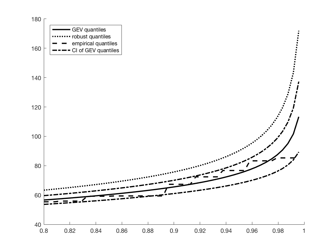
(a) Quantile plots for rainfall data, Eg. 1

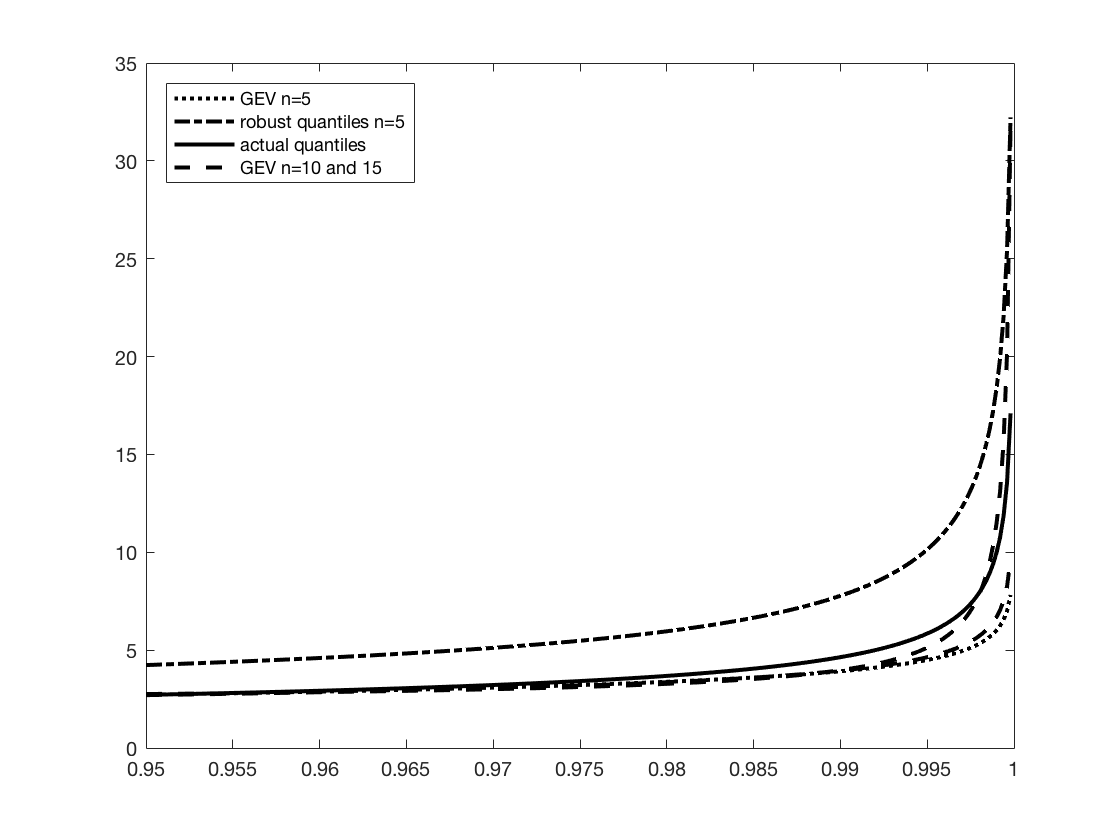
(b) Quantile plots for Pareto data, Eg. 2

Example 2.

In this example, we are provided with 100 independent samples of a Pareto random variable satisfying $P\{X>x\}=1-F(x)=1\wedge x^{-3}.$ As before, the objective is to compute quantiles $F^{\leftarrow}(p)$ for values of $p$ close to 1. As the entire probability distribution is known beforehand, this offers an opportunity to compare the quantile estimates returned by our algorithm with the actual quantiles. Unlike Example 1, the data in this example does not present a natural means to choose block sizes. As a first choice, we choose block size $n=5$ and perform routine computations as in Algorithm 1 to obtain a reference GEV model $P_{{}_{\mathnormal{GEV}}}$ with parameters $\gamma_{0}=0.11,a_{0}=0.58,b_{0}=1.88,$ and corresponding tolerance parameters $\alpha=1.5$ and $\delta=0.8.$ Then the worst-case quantile estimate $F_{\alpha}^{\leftarrow}(p^{n})=\sup\{G^{\leftarrow}(p^{n}):D_{\alpha}(G,P_{{}_{\mathnormal{GEV}}})\leq\delta\}$ is immediately calculated for various values of $p$ close to 1, and the result is plotted (in the dotted line) against the true quantiles $F^{\leftarrow}(p)=(1-p)^{-1/3}$ (in the solid line) in Figure 1(b). These can, in turn, be compared with the quantile estimates $x_{p}$ (in the solid line) due to traditional GEV extrapolation with reference model $P_{{}_{\mathnormal{GEV}}}.$ Recall that the initial choice for block size, $n=5,$ was arbitrary. One can perhaps choose a different block size, which will result in a different model for corresponding block-maximum $M_{n}.$ For example, if we choose $n=10,$ the respective GEV model for $M_{10}$ has parameters $\gamma_{0}=0.22,a_{0}=0.55$ and $b_{0}=2.3.$ Whereas, if we choose $n=15,$ the GEV model for $M_{15}$ has parameters $\gamma_{0}=0.72,a_{0}=0.32\text{ and }b_{0}=2.66.$ When considering the shape parameters, these models are different, and subsequently, the corresponding quantile estimates (plotted using dashed lines in Figure 1(b)) are also different. However, as it can be inferred from Figure 1(b), the robust quantile estimates (in the dotted line) obtained by running Algorithm 1 forms a good upper bound to the actual quantiles $F^{\leftarrow}(p),$ as well as to the quantile estimates due to different GEV extrapolations from different block sizes $n=10$ and 15.

Example 3.

The objective of this example is to demonstrate the applicability of Algorithm 1 in an instance where the traditional extrapolation techniques tend to not yield stable estimates. For this purpose, we use N = 2000 independent samples of the random variable $Y=X+50\mathbf{1}(X>5)$ as input to the maximum likelihood based GEV model estimation, with the aim of calculating the extreme quantile $F^{\leftarrow}(0.999).$ Here, $F$ denotes the distribution function of random variable $Y,$ and $X$ is a Pareto random variable with distribution $\max(1-x^{-1.1},0).$ The quantile estimates (and the corresponding 95% confidence intervals) output by this traditional GEV estimation procedure, for various choices of block sizes, is displayed with the solid line in Figure 2. Even for modestly large block size choices, it can be observed that the 95% confidence regions obtained from the calibrated GEV models are far below the true quantile drawn in the dashed line. This underestimation is perhaps because of the sudden shift of samples of block-maxima $M_{n}$ from a value less than 5 to a value larger than 55 (recall that the distribution $F$ assigns zero probability to the interval $(5,55)$).

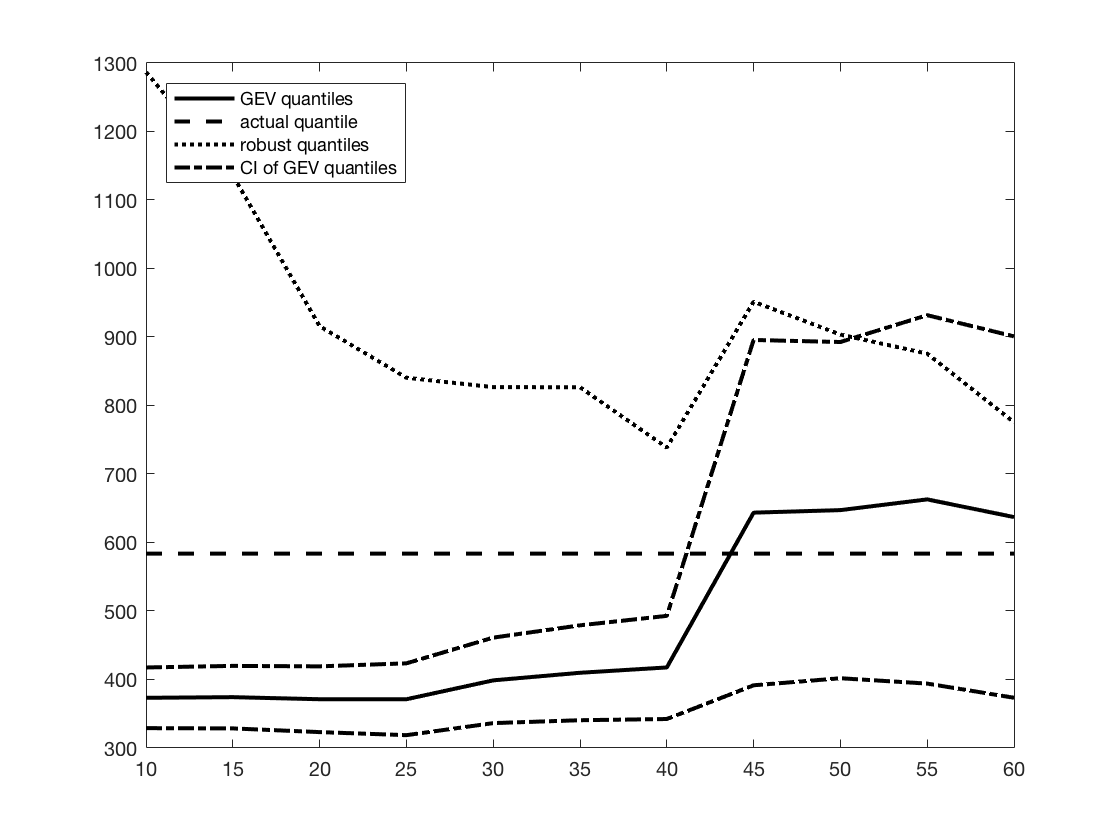
Figure 2. Plot for Example 3, instability in estimated quantile $F^{\leftarrow}(0.999)$

Next, we use Algorithm 1 to yield an upper bound that is robust against model errors. Unlike previous examples where standard errors are used to calculate the suitable $\alpha,$ in this example, we use the domain knowledge that the samples of $Y$ have finite mean, which means, $\gamma^{\ast}\leq 1.$ Assuming no additional information, we resort to the conservative choice $\gamma^{\ast}=1.$ The dashed curve in Figure 2 corresponds to the upper bound on $F^{\leftarrow}(0.999)$ output by Algorithm 1. We note the following observations: First, the worst case estimates output by Algorithm 1 indeed act as an upper bound for the true quantile (drawn in solid line), irrespective of the block-size chosen and the baseline GEV model used. Second, for block-sizes smaller than $n=45,$ it appears that the calibrated baseline GEV models are not representative enough of the distribution of $M_{n},$ and hence higher the value of $\delta$ for these choices of block sizes. Understandably, this results in a conservative worst case estimate for the smaller choices of block sizes. However, we argue that the overall procedure is not discouragingly conservative, by observing that the spread of 95% confidence region for block size choices $n=$ 50 to 60 (where the traditional GEV calibration appears correct) is comparable to the difference between the true quantile and the worst-case estimate produced by Algorithm 1 for majority of block size choices (from $n=$ 20 to 60).

Example 4.

In this example we consider the St. Petersburg distribution, which is not in the maximum domain of attraction of any GEV distribution (see e.g. [11]). Recall that $X$ is St.Petersburg distributed if

(24) $$P\{X=2^{k}\}=2^{-k},\quad k=1,2,\dots$$

Note that the St. Petersburg distribution takes large values with tiny probability. Let $B$ denote a Bernoulli random variable with parameter $1/5$. In addition let $W$ be exponentially distributed with mean $8$ and define $Z=B\cdot X+W.$ Suppose we have 5000 data points from the distribution of $Z$. Similar to the previous example, we want to estimate its quantile $F^{\leftarrow}(0.999)$.

Here we demonstrate another approach to choose the parameter $\alpha$. The idea, as described earlier in Item 3) is to first choose a tail probability level $q$ for which $F^{\leftarrow}(q)$ can be accurately estimated from the whole data set. For our example, we take $q=0.99$ and compute the plug-in estimate $F^{\leftarrow}(q)$ from the empirical distribution. Then we independently divide the given data set uniformly at random into $10$ batches each of size $625$ samples (corresponding to a scale-down factor = 8). We employ the procedure Rob-Estimator$(q,\alpha)$ for various values of $\alpha$ on each of these 10 sub-sampled mini-batches independently, and choose the largest value of $\alpha$ such that the robust estimates from each of the 10 sub-samples cover the earlier plug-in estimate $F^{\leftarrow}(0.99)$. The specific details for this example are as follows:

1) The plug-in estimate for $F^{\leftarrow}(0.99)$ from the given 5000 samples is 44.9. Note that with 5000 samples, this estimate from empirical distribution is with reasonably high confidence.

2) Resample the data into 10 mini-batches of size 5000/8 = 625 samples. With blocksize = 20 we utilize the procedure Rob-Estimator$(0.99,\alpha)$ on each of the 10 mini-batches to choose the largest $\alpha$ such that the respective robust estimates from all the 10 sub-sampled mini-batches cover the empirical estimate of $F^{\leftarrow}(0.99)$ obtained from step 1). This approach leads us to the choice of $\alpha=4.47$. Computing block maxima from blocks of samples with size = 48, the subsequent robust upper bound from the procedure Rob-Estimator$(0.999,4.47)$ turns out to be $652.90,$ which covers the true quantile, $F^{\leftarrow}(0.999)=268.27.$ In contrast, the $95\%$-confidence interval of GEV estimate is $[93.81,201.60]$, which fails to cover the true quantile.

This approach incorporates the trade-off between the choice of $\alpha$ and $\delta$. Large values of $\alpha$ may be desirable because they generate less conservative upper bounds. But Step 2) avoids picking too large values of $\alpha$, because too large values of $\alpha$, combined with the corresponding estimators for $\delta$ empirically do not lead to good coverage for $F^{\leftarrow}(0.99)$. Therefore this cross-validation-like procedure automatically incorporates the trade-off between the choice of hyperparameters $\alpha$ and $\delta$.

6. Proofs of main results

In this section, we provide proofs of Theorems 5 and 6, along with proofs of Propositions 4, 8 and c).

6.1. Proof of Proposition 4

By definition, $F_{\alpha,\delta}(x)$ is non-decreasing in $x.$ Since $F_{\alpha,\delta}(x)\leq P_{ref}(-\infty,x),$ we have $\lim_{x\rightarrow-\infty}F_{\alpha,\delta}(x)=0.$ In addition, we have from Corollary 1 that $\bar{F}_{\alpha,\delta}(x)=\theta_{x}P_{ref}(x,\infty),$ where $\theta_{x}$ satisfies (18). Since $P_{ref}(x,\infty)\phi_{\alpha}(\theta_{x})\leq\bar{\delta}$ (follows from (18)), we have $\theta_{x}\leq\phi_{\alpha}^{-1}(\bar{\delta}/P_{ref}(x,\infty)),$ where $\phi_{\alpha}^{-1}(\cdot)$ is the inverse function of $\phi_{\alpha}(\cdot)$ (recall the defintion of $\phi_{\alpha}(\cdot)$ in (13) to see that the inverse is well-defined for every $\alpha\geq 1$). As a result,

(25) $$\bar{F}_{\alpha,\delta}(x)\leq\phi_{\alpha}^{-1}\left(\frac{\bar{\delta}}{P_{ref}(x,\infty)}\right)P_{ref}(x,\infty).$$

If we let $W(x)$ denote the product log function, then $\phi^{-1}_{\alpha}(u)=u^{-1/\alpha}$ when $\alpha>1$ and $\phi^{-1}_{\alpha}(u)=u/W(u)$ when $\alpha=1.$ Consequently for any $\alpha\geq 1,$ $\epsilon\phi_{\alpha}^{-1}(1/\epsilon)\rightarrow 0$ as $\epsilon\rightarrow 0.$ As a result, $\lim_{x\rightarrow\infty}\bar{F}_{\alpha,\delta}(x)=0$ for any choice of $\alpha\geq 1$ and $\delta>0.$ Thus $\lim_{x\rightarrow\infty}F_{\alpha,\delta}(x)=1.$

To show that $F_{\alpha,\delta}(x)$ is right-continuous, we first see that

$$F_{\alpha,\delta}(x+\epsilon)-F_{\alpha,\delta}(x) =\sup_{P:D_{\alpha}(P,P_{ref})\leq\delta}P(x,\infty)-\sup_{P:D_{\alpha}(P,P_{ref})\leq\delta}P(x+\epsilon,\infty)$$

$$\leq\sup_{P:D_{\alpha}(P,P_{ref})\leq\delta}P(x,x+\epsilon],$$

for any $\epsilon>0,$ for every choice of $\delta>0,\alpha\geq 1$ and $P_{ref}.$ Following the same reasoning as in (25), we obtain that

$$\sup_{P:D_{\alpha}(P,P_{ref})\leq\delta}P(x,x+\epsilon]\leq\phi_{\alpha}^{-1}\left(\frac{\bar{\delta}}{P_{ref}(x,x+\epsilon]}\right)P_{ref}(x,x+\epsilon],$$

for which the right hand side vanishes when $\epsilon\rightarrow 0.$ As a result, $F_{\alpha,\delta}(x)$ is right-continuous as well, thus verifying all the properties required to prove that $F_{\alpha,\delta}(\cdot)$ is a cumulative distribution function. $\Box$

6.2. Proofs of Theorems 5 - 6

The following technical result, Lemma 12, is useful for proving Theorem 6. Given $\alpha\geq 1,$ $u\in(0,1)$ and $\bar{\delta}<\delta_{thr}(u),$ define

(26) $$h(u):=u\theta(u),$$

where $\theta(u)$ is a value of $\theta$ satisfying

(27) $$u\theta^{\alpha}+(1-u)\left(\frac{1-\theta u}{1-u}\right)^{\alpha}=\bar{\delta}.$$

Lemma 12.

For any $\alpha>1$ and $\bar{\delta}>1,$

$$\lim_{u\searrow 0}\frac{\theta(u)}{h^{\prime}(u)}=\frac{\alpha}{\alpha-1}\quad\text{ and }\quad\lim_{u\searrow 0}\frac{h(u)h^{\prime\prime}(u)}{\left(h^{\prime}(u)\right)^{2}}=-\frac{1}{\alpha-1}.$$

Proof of Lemma 12.

For $u\in(0,1),$ $\theta(u)$ satisfying (27) exists if $u$ is small enough such that $\delta_{thr}(u):=u\phi_{\alpha}(1/u)\geq\bar{\delta}$ (see Corollary 1). For all such small enough $u,$ an application of implicit function theorem gives that,

$$\theta^{\prime}(u)=\frac{(1-u)^{\alpha}\theta^{\alpha}(u)-(1-u\theta(u))^{\alpha}+\alpha(1-\theta(u))(1-u\theta(u))^{\alpha-1}}{\alpha(1-u)u[(1-u\theta(u))^{\alpha-1}-(1-u)^{\alpha-1}\theta^{\alpha-1}(u)]},$$

and consequently,

$$h^{\prime}(u)=\frac{(\alpha-1)[(1-u\theta(u))^{\alpha}-(1-u)^{\alpha}\theta^{\alpha}(u)]}{\alpha(1-u)[(1-u\theta(u))^{\alpha-1}-(1-u)^{\alpha-1}\theta^{\alpha-1}(u)]}.$$

Since $u\theta(u)\leq u\phi_{\alpha}^{-1}(\bar{\delta}/u)$ (see (25)), we have $u\theta(u)\rightarrow 0$ as $u\searrow 0.$ Moreover, since $\theta(u)\geq(\bar{\delta}-(1-u)^{-(\alpha-1)})/u$ (from (27)), we have that $\theta(u)\rightarrow\infty,$ as $u\searrow 0.$ Combining these observations with the above expression for $h^{\prime}(u),$ we arrive at the first conclusion that $\lim_{u\searrow 0}\theta(u)/h^{\prime}(u)=\alpha/(\alpha-1).$

To verify the second limiting statement, we proceed by rewriting as follows:

$$\frac{h(u)h^{\prime\prime}(u)}{\left(h^{\prime}(u)\right)^{2}}=\frac{\theta(u)}{h^{\prime}(u)}\frac{h^{\prime\prime}(u)}{\theta^{\prime}(u)}\frac{u\theta^{\prime}(u)}{h^{\prime}(u)}$$

We know from the above that ${\theta(u)}/{h^{\prime}(u)}$ converges to ${\alpha}/(\alpha-1)$, as $u\searrow 0;$ and by l’Hôspital’s rule, we have ${h^{\prime\prime}(u)}/{\theta^{\prime}(u)}$ converges to $(\alpha-1)/\alpha.$ Finally,

$$\frac{u\theta^{\prime}(u)}{h^{\prime}(u)} =\frac{u\theta^{\prime}(u)}{\theta(u)+u\theta^{\prime}(u)}$$

$$=\frac{(1-u)^{\alpha}\theta^{\alpha}(u)-(1-u\theta(u))^{\alpha}+\alpha(1-\theta(u))(1-u\theta(u))^{\alpha-1}}{(\alpha-1)[(1-u\theta(u))^{\alpha}-(1-u)^{\alpha}\theta^{\alpha}(u)]},$$

which converges to $-\frac{1}{\alpha-1}$, since $u\theta(u)\rightarrow 0$ as $u\searrow 0$.Combining the above observations, the verification of the second conclusion that ${h(u)h^{\prime\prime}(u)}/{(h^{\prime}(u))^{2}}\rightarrow-1/(\alpha-1)$ is complete. $\Box$ ∎

Proof of Theorem 6

Our goal is to determine the maximum domain of attraction membership of $\bar{F}_{\alpha,\delta}(x)=\sup\{P(x,\infty):D_{\alpha}(P,P_{{}_{\mathnormal{ref}}})\leq\delta\}.$ For brevity, let $\bar{F}(x):=P_{{}_{\mathnormal{ref}}}(x,\infty).$ Then for values of $x$ such that $P_{{}_{\mathnormal{ref}}}(x,\infty)$ small enough, we have from Corollary 1 that $\bar{F}_{\alpha,\delta}(x)=h(\bar{F}(x)).$ Since $\bar{F}(\cdot)$ satisfies the regularity conditions in the statement of Proposition 1, we have

(28) $$\lim_{x\uparrow x_{F}^{\ast}}\frac{\bar{F}(x)\bar{F}^{\prime\prime}(x)}{\left(\bar{F}^{\prime}(x)\right)^{2}}=\gamma_{ref}+1,$$

and the following from elementary calculus:

$$\bar{F}_{\alpha,\delta}^{\prime}(x) ={h}^{\prime}(\bar{F}(x))\bar{F}^{\prime}(x)\text{ and}$$

$$\bar{F}_{\alpha,\delta}^{\prime\prime}(x) =h^{\prime\prime}(\bar{F}(x))(\bar{F}^{\prime}(x))^{2}+h^{\prime}(\bar{F}(x))\bar{F}^{\prime\prime}(x).$$

Combining these observations with the definition in (26), we arrive at,

(29) $$\frac{\bar{F}_{\alpha,\delta}(x)\bar{F}_{\alpha,\delta}^{\prime\prime}(x)}{\left(\bar{F}_{\alpha,\delta}^{\prime}(x)\right)^{2}}=\frac{h(\bar{F}(x))h^{\prime\prime}(\bar{F}(x))}{\left(h^{\prime}(\bar{F}(x))\right)^{2}}+\frac{\theta(\bar{F}(x))}{h^{\prime}(\bar{F}(x))}\left(\frac{\bar{F}(x)\bar{F}^{\prime\prime}(x)}{\left(\bar{F}^{\prime}(x)\right)^{2}}\right).$$

Since $\bar{F}(x)\rightarrow 0$ as $x\rightarrow x_{F}^{\ast},$ it follows from Lemma 12, (29) and (28) that,

$$\lim_{x\uparrow x_{F}^{\ast}} \left(\frac{1-F_{\alpha,\delta}}{F_{\alpha,\delta}^{\prime}}\right)^{\prime}(x)=\lim_{x\uparrow x_{F}^{\ast}}\frac{\bar{F}_{\alpha,\delta}(x)\bar{F}_{\alpha,\delta}^{\prime\prime}(x)}{\left(\bar{F}_{\alpha,\delta}^{\prime}(x)\right)^{2}}-1$$

$$=\lim_{u\searrow 0}\frac{h(u)h^{\prime\prime}(u)}{\left(h^{\prime}(u)\right)^{2}}+\lim_{u\searrow 0}\frac{\theta(u)}{h^{\prime}(u)}\lim_{u\searrow 0}\frac{\bar{F}(x)\bar{F}^{\prime\prime}(x)}{\left(\bar{F}^{\prime}(x)\right)^{2}}-1$$

$$=-\frac{1}{\alpha-1}+\frac{\alpha}{\alpha-1}\left(\gamma_{ref}+1\right)-1=\frac{\alpha}{\alpha-1}\gamma_{ref}.$$

Thus, due to the characterization in Proposition 1, we have that $F_{\alpha,\delta}$ lies in the maximum domain of attraction of $G_{\gamma^{\ast}}.$ $\Box$

Proof of Theorem 5

Theorem 5 follows as a simple corollary of Theorem 6, once we verify that any GEV model $G(x):=P_{{}_{\mathnormal{GEV}}}(-\infty,x]$ satisfies $G^{\prime}(x)>0$ and $G^{\prime\prime}(x)$ exists in a left neighborhood of $x_{G}^{*}=\sup\{x:G(x)<1\},$ along with the property that

$$\lim_{x\uparrow x_{G}^{*}}\left(\frac{1-G}{G^{\prime}}\right)^{\prime}(x)=\gamma_{{}_{\mathnormal{ref}}},$$

where $\gamma_{{}_{\mathnormal{ref}}}$ is the shape parameter of $G.$ Such a GEV model satisfies $G(x)=G_{\gamma_{\textnormal{ref}}}(ax+b)$ for some scaling and translation constants $a$ and $b.$ Therefore, it is enough to verify these properties only for $G(x)=G_{\gamma_{\textnormal{ref}}}(x).$ Once we recall the definition of $G_{\gamma}$ in (4), the desired properties are elementary exercises in calculus. $\Box$

6.3. Proofs of Propositions 8 - c)

Given $u\in(0,1)$ and $\bar{\delta}<\delta_{thr}(u),$ let $\theta(u)$ be a value of $\theta$ that solves the equation,

(30) $$u\theta\log\theta+(1-\theta u)\log\frac{1-\theta u}{1-u}=\bar{\delta}.$$

Define $h(u):=u\theta(u)$ (as in the proof of Theorem 6, see (26)). The following technical result, Lemma 13, is useful for proving Proposition 8.

Lemma 13.

For any $\bar{\delta}>1,$

$$\lim_{u\searrow 0}\frac{\theta(u)}{h^{\prime}(u)}+\frac{h(u)h^{\prime\prime}(u)}{\left(h^{\prime}(u)\right)^{2}}=2.$$

Proof of Lemma 13.

For $u\in(0,1),$ $\theta(u)$ satisfying (27) exists if $u$ is small enough such that $\delta_{thr}(u):=u\phi_{\alpha}(u)\geq\bar{\delta}$ (see Corollary 1). For all such small enough $u,$ an application of implicit function theorem gives that,

$$\theta^{\prime}(u)=\frac{\theta(u)-1}{u(1-u)L(u)}-\frac{\theta(u)}{u},\quad\text{ where }L(u):=\log\frac{\theta(u)(1-u)}{1-u\theta(u)}.$$

∎

Since $h^{\prime}(u)=\theta(u)+u\theta^{\prime}(u),$ it follows that,

(31) $$\frac{\theta(u)-1}{h^{\prime}(u)}=L(u)(1-u).$$

Differentiating both sides and multiplying by $h(u),$ we obtain,

$$\frac{h(u)\theta^{\prime}(u)}{h^{\prime}(u)}-\left(\theta(u)-1\right)\frac{h(u)h^{\prime\prime}(u)}{\left(h^{\prime}(u)\right)^{2}}=u\theta(u)\left(L^{\prime}(u)(1-u)-L(u)\right).$$

Since the first term in the left hand side above simplifies to

$$\frac{h(u)\theta^{\prime}(u)}{h^{\prime}(u)}=\theta(u)\left(1-\frac{1-u}{1-1/\theta(u)}L(u)\right),$$

we obtain that,

(32) $$\left(1-\frac{1}{\theta(u)}\right)\frac{h(u)h^{\prime\prime}(u)}{\left(h^{\prime}(u)\right)^{2}}=1-\frac{(1-u)L(u)}{1-1/\theta(u)}+uL(u)-u(1-u)L^{\prime}(u).$$

Differentiating $L(u),$ we obtain,

$$\left(1-u\theta(u)\right)L^{\prime}(u)=\frac{\theta^{\prime}(u)}{\theta(u)}+\frac{\theta(u)-1}{1-u}.$$

Substituting this observation in (32), we obtain

$$\left(1-\frac{1}{\theta(u)}\right)\frac{h(u)h^{\prime\prime}(u)}{\left(h^{\prime}(u)\right)^{2}}$$

$$\qquad=1+\left(u-\frac{1-u}{1-1/\theta(u)}\right)L(u)-\frac{1-u}{1-u\theta(u)}\left(\frac{u\theta^{\prime}(u)}{\theta(u)}+\frac{u(\theta(u)-1)}{1-u}\right).$$

Combining this observation with that in (31), we obtain,

$$\left(1-\frac{1}{\theta(u)}\right)\left(\frac{\theta(u)}{h^{\prime}(u)}+\frac{h(u)h^{\prime\prime}(u)}{\left(h^{\prime}(u)\right)^{2}}\right)$$

$$\qquad=1-\frac{1-u\theta(u)}{\theta(u)-1}L(u)-\frac{1-u}{1-u\theta(u)}\left(\frac{1-1/\theta(u)}{(1-u)L(u)}-1+\frac{u(\theta(u)-1)}{1-u}\right).$$

Since $u\theta(u)\leq u\phi_{1}^{-1}(\bar{\delta}/u)$ (see (25)), we have $u\theta(u)\rightarrow 0$ as $u\searrow 0.$ Moreover, since $\theta(u)\geq\phi^{-1}((\bar{\delta}+\log(1-u))/u)$ (from (30)), we have that $\theta(u)\rightarrow\infty,$ as $u\searrow 0.$ Therefore, we have from the above displayed equation that,

$$\lim_{u\searrow 0}1\times\left(\frac{\theta(u)}{h^{\prime}(u)}+\frac{h(u)h^{\prime\prime}(u)}{\left(h^{\prime}(u)\right)^{2}}\right)$$

$$\qquad=1-(1-0)\lim_{u\searrow 0}\frac{L(u)}{\theta(u)-1}-\frac{1-0}{1-0}\left(\frac{1-0}{1\times\lim_{u\searrow 0}L(u)}-1-\frac{0}{1}\right).$$

It follows from the definition of $L(u)$ that $L(u)\rightarrow\infty$ as $u\searrow 0;$ due to L’Hôspital’s rule, we also obtain $\lim_{u\searrow 0}L(u)/(\theta(u)-1)=0.$ This verifies the statement of Lemma 13. $\Box$

Proof of Proposition 8

Our objective is to identify the maximum domain of attraction memberiship of the tail probability function,

$$\bar{F}_{1,\delta}(x):=\sup\{P(x,\infty):D_{1}(P,G_{0})\leq\delta\}.$$

For brevity, let $\bar{G}_{0}(x):=1-G_{0}(x).$ Then for values of $x$ such that $\bar{G}_{0}(x)$ small enough, we have from Corollary 1 that $\bar{F}_{1,\delta}(x)=h(\bar{G}_{0}(x)).$ Since $\bar{G}_{0}(\cdot)$ satisfies the regularity conditions in the statement of Proposition 1, we have

(33) $$\lim_{x\uparrow\infty}\frac{\bar{G}_{0}(x)\bar{G}_{0}^{\prime\prime}(x)}{\left(\bar{G}_{0}^{\prime}(x)\right)^{2}}=1,$$

Then, as in the proof of Theorem 6, we have from Lemma 13, (33),(29) that,

$$\lim_{x\rightarrow\infty} \left(\frac{1-F_{1,\delta}}{F_{1,\delta}^{\prime}}\right)^{\prime}(x)=\lim_{x\rightarrow\infty}\frac{\bar{F}_{1,\delta}(x)\bar{F}_{1,\delta}^{\prime\prime}(x)}{\left(\bar{F}_{1,\delta}^{\prime}(x)\right)^{2}}-1$$

$$=\lim_{x\rightarrow\infty}\frac{h(\bar{G}_{0}(x))h^{\prime\prime}(\bar{G}_{0}(x))}{\left(h^{\prime}(\bar{G}_{0}(x))\right)^{2}}+\frac{\theta(\bar{G}_{0}(x))}{h^{\prime}(\bar{G}_{0}(x))}\frac{\bar{G}_{0}(x)\bar{G}_{0}^{\prime\prime}(x)}{\left(\bar{G}_{0}^{\prime}(x)\right)^{2}}-1$$

$$=2-1=1.$$

Thus, due to the characterization in Proposition 1, we have that $F_{1,\delta}$ lies in the maximum domain of attraction of $G_{1}.$ $\Box$

Proof of Proposition c)

First, we treat the case $\gamma_{{}_{\mathnormal{ref}}}=0$: Consider the probability density function $f(x)=c(x\log x)^{-2}\mathbf{1}(x\geq 2),$ where $c$ is a normalizing constant that makes $\int f(x)dx=1.$ In addition, let $g(x)=G_{0}^{\prime}(x)$ denote the probability density function corresponding to the distribution $G_{0}.$ Clearly,

$$D_{1}(f,g) =\int f(x)\log\left(\frac{f(x)}{g(x)}\right)dx$$

$$=c\int_{2}^{\infty}(x\log x)^{-2}\log\left(\frac{c(x\log x)^{-2}}{\exp(-\exp(-x))\exp(-x)}\right)dx$$

$$\leq\int_{2}^{\infty}\frac{x+\exp(-x)+\log c}{x^{2}\log^{2}x}dx<\infty.$$

Next, consider the family of densities $\{h_{a}:a\in[0,1]\},$ where

(34) $$h_{a}:=af+(1-a)g.$$

Since $D_{1}(h_{0},g)=0,$ due to the continuity of $D_{1}(h_{a},g)$ with respect to $a,$ there exists an $\bar{a}\in(0,1)$ such that $D_{1}(h_{\bar{a}},g)\leq\delta.$ Then,

$$\int_{x}^{\infty}h_{\bar{a}}(u)du =\int_{x}^{\infty}\left(\bar{a}f+(1-\bar{a})g\right)(u)du$$

$$\geq\bar{a}\int_{x}^{\infty}\frac{c}{u^{2}\log^{2}u}du=\frac{\bar{a}c+o(1)}{x\log^{2}x},$$

The asymptotic equivalence used above in the last equality is due to Karamata’s theorem (see Theorem 1 in Chapter VIII.9 of [10]). This demonstrates the existence of a probability distribution $P$ and constants $c_{0},x_{0}$ such that $P(x,\infty)\geq c_{0}x^{-1}\log^{-2}x$ for all $x\geq x_{0}.$

Next, we treat the case $\gamma_{{}_{\mathnormal{ref}}}\neq 0$: Consider the probability measure $Q$ whose Radon-Nikodym derivative is given by,

$$\frac{dQ}{dG_{\gamma_{{}_{\mathnormal{ref}}}}}(x)=\phi_{1}^{-1}\left(\frac{c}{(1-G_{\gamma_{{}_{\mathnormal{ref}}}}(x))(1-\log(1-G_{\gamma_{{}_{\mathnormal{ref}}}}(x)))^{2}}\right),$$

for a suitable positive constant $c$. Here $\phi_{1}^{-1}(\cdot)$ denotes the inverse function of $\phi_{1}(x).$ Then $D_{1}(Q,P_{{}_{\mathnormal{ref}}})<\infty$ because of the change of variable from $x$ to $u$ via the relationship $u=1-G_{\gamma_{{}_{\mathnormal{ref}}}}(x)$ in the integration below:

$$\int\phi_{1}\left(\frac{dQ}{dG_{\gamma_{{}_{\mathnormal{ref}}}}}\right)dG_{\gamma_{{}_{\mathnormal{ref}}}}=\int_{0}^{1}\frac{c}{u(1-\log u)^{2}}du<\infty.$$

Let $g(x):=G_{\gamma_{{}_{\mathnormal{ref}}}}^{\prime}(x)$ and $f$ denote the probability density of the measure $Q.$ Consider the family of probability density functions $\{h_{a}:a\in[0,1]\},$ where $h_{a}$ is defined in $\eqref{defn:ha}.$ Since $D_{1}(h_{0},g)=0,$ due to the continuity of $D_{1}(h_{a},g)$ with respect to $a,$ there exists an $\bar{a}\in(0,1)$ such that $D_{1}(h_{\bar{a}},g)\leq\delta.$ Moreover, if we let $A(t)=\phi_{1}^{-1}(c(1-\log t)^{-2}/t),$ then observe that there exists a $t_{0}$ such that $A(t)$ is decreasing in the interval $(0,t_{0}).$ Therefore,

$$\int_{x}^{\infty}h_{\bar{a}}(u)du \geq\bar{a}\int_{x}^{\infty}\frac{f(u)}{g(u)}g(u)du=\bar{a}\int_{x}^{\infty}A(1-G_{\gamma_{{}_{\mathnormal{ref}}}}(u))g(u)du$$

$$\geq\bar{a}A(1-G_{\gamma_{{}_{\mathnormal{ref}}}}(x))\int_{x}^{\infty}g(u)du=\bar{a}A(1-G_{\gamma_{{}_{\mathnormal{ref}}}}(x))(1-G_{\gamma_{{}_{\mathnormal{ref}}}}(x)),$$

for all $x$ large enough. To proceed further, observe that

$$1-G_{\gamma_{\textnormal{ref}}}(x)\geq\bar{c}(1+\gamma_{{}_{\mathnormal{ref}}}x)^{-1/\gamma_{{}_{\mathnormal{ref}}}},$$

for some constant $\bar{c}<1$ and all $x$ close enough to the right endpoint $x^{*}_{{}_{G}}:=\sup\{x:G_{\gamma_{\textnormal{ref}}}(x)<1\}.$ In addition, $tA(t)$ strictly decreases to 0 as $t$ decreases to 0. Therefore, for all $x$ close to the right endpoint $x^{*}_{G}:=\sup\{x:G_{\gamma_{\textnormal{ref}}}(x)<1\},$ it follows that

$$\int_{x}^{\infty}h_{\bar{a}}(u)du\geq A\left(\bar{c}(1+\gamma_{{}_{\mathnormal{ref}}}x)^{-1/\gamma_{{}_{\mathnormal{ref}}}}\right)\bar{c}(1+\gamma_{{}_{\mathnormal{ref}}}x)^{-1/\gamma_{{}_{\mathnormal{ref}}}}.$$

Since $\phi_{1}^{-1}(u)\geq u/\log u$ for large enough $u,$ $A(t)\geq ac{t^{-1}\left(1-\log t\right)^{-2}\log^{-1}\left(c/t\right)},$ for all $t$ close to 0. As a result, there exists a constant $c^{\prime}$ such that $tA(t)\geq c^{\prime}(1-\log t)^{-3}$ for all $t$ sufficiently close to 0. This allows us to write

$$\int_{x}^{\infty}h_{\bar{a}}(u)du \geq c^{\prime}(1-\log(\bar{c}(1+\gamma_{{}_{\mathnormal{ref}}}x)^{-1/\gamma_{{}_{\mathnormal{ref}}}}))^{-3}$$

$$=c^{\prime}(1+\log(\bar{c}^{1/\gamma_{{}_{\mathnormal{ref}}}}(1+\gamma_{{}_{\mathnormal{ref}}}x))/\gamma_{{}_{\mathnormal{ref}}})^{-3},$$

for $x$ sufficiently close $x_{{}_{G}}^{\ast},$ thus verifying the statement in cases (a) and (c) where $\gamma_{{}_{\mathnormal{ref}}}\neq 0.$ This completes the proof of Proposition c). $\Box$

References

• [1] A. Ahmadi-Javid. Entropic value-at-risk: A new coherent risk measure. Journal of Optimization Theory and Applications, 155(3):1105–1123, Dec 2012.
• [2] R. Atar, K. Chowdhary, and P. Dupuis. Robust bounds on risk-sensitive functionals via Rényi divergence. SIAM/ASA J. Uncertain. Quantif., 3(1):18–33, 2015.
• [3] A. Ben-Tal, D. den Hertog, A. D. Waegenaere, B. Melenberg, and G. Rennen. Robust solutions of optimization problems affected by uncertain probabilities. Management Science, 59(2):341–357, 2013.
• [4] T. Breuer and I. Csiszár. Measuring distribution model risk. Mathematical Finance, 2013.
• [5] S. Coles. An introduction to statistical modeling of extreme values. Springer Series in Statistics. Springer-Verlag London, Ltd., London, 2001.
• [6] S. G. Coles and J. A. Tawn. A bayesian analysis of extreme rainfall data. Journal of the Royal Statistical Society. Series C (Applied Statistics), 45(4):pp. 463–478, 1996.
• [7] L. de Haan and A. Ferreira. Extreme value theory. Springer Series in Operations Research and Financial Engineering. Springer, New York, 2006. An introduction.
• [8] P. Dupuis, M. R. James, and I. Petersen. Robust properties of risk-sensitive control. Mathematics of Control, Signals and Systems, 13(4):318–332, 2000.
• [9] P. Embrechts, C. Klüppelberg, and T. Mikosch. Modelling extremal events, volume 33 of Applications of Mathematics (New York). Springer-Verlag, Berlin, 1997. For insurance and finance.
• [10] W. Feller. An introduction to probability theory and its applications. Vol. II. John Wiley & Sons, Inc., New York-London-Sydney, 1966.
• [11] G. Fukker, L. Gyorfi, and P. Kevei. Asymptotic behavior of the generalized st.petersburg sum conditioned on its maximum. Bernoulli 22(2),1026-1054, 2016.
• [12] P. Glasserman and X. Xu. Robust risk measurement and model risk. Quantitative Finance, 14(1):29–58, 2014.
• [13] M. Gupta and S. Srivastava. Parametric bayesian estimation of differential entropy and relative entropy. Entropy, 12(4):818, 2010.
• [14] L. P. Hansen and T. J. Sargent. Robust control and model uncertainty. The American Economic Review, 91(2):pp. 60–66, 2001.
• [15] P. Jorion. Value at Risk, 3rd Ed.: The New Benchmark for Managing Financial Risk. McGraw-Hill Education, 2006.
• [16] M. R. Leadbetter, G. Lindgren, and H. Rootzén. Extremes and related properties of random sequences and processes. Springer Series in Statistics. Springer-Verlag, New York-Berlin, 1983.
• [17] F. Liese and I. Vajda. Convex statistical distances. Teubner Texts in Mathematics. BSB B. G. Teubner Verlagsgesellschaft, Leipzig, 1987.
• [18] X. Nguyen, M. Wainwright, and M. Jordan. Estimating divergence functionals and the likelihood ratio by convex risk minimization. IEEE Transactions on Information Theory, 56(11):5847–5861, Nov 2010.
• [19] X. Nguyen, M. J. Wainwright, and M. I. Jordan. On surrogate loss functions and f-divergences. Ann. Statist., 37(2):876–904, 04 2009.
• [20] B. Póczos and J. Schneider. On the estimation of alpha-divergences. In AISTATS, 2011.
• [21] A. Rényi. On measures of entropy and information. In Proc. 4th Berkeley Sympos. Math. Statist. and Prob., Vol. I, pages 547–561. Univ. California Press, Berkeley, Calif., 1961.
• [22] S. I. Resnick. Extreme values, regular variation and point processes. Springer Series in Operations Research and Financial Engineering. Springer, New York, 2008. Reprint of the 1987 original.
• [23] Y.-L. Tsai, D. J. Murdoch, and D. J. Dupuis. Influence measures and robust estimators of dependence in multivariate extremes. Extremes, 14(4):343–363, 2010.
• [24] Q. Wang, S. R. Kulkarni, and S. Verdu. Divergence estimation for multidimensional densities via $k$-nearest-neighbor distances. IEEE Transactions on Information Theory, 55(5):2392–2405, May 2009.