On the quantum no-signalling assisted
zero-error classical simulation cost of
non-commutative bipartite graphs

Abstract

Using one channel to simulate another exactly with the aid of quantum no-signalling correlations has been studied recently. The one-shot no-signalling assisted classical zero-error simulation cost of non-commutative bipartite graphs has been formulated as semidefinite programms [Duan and Winter, IEEE Trans. Inf. Theory 62, 891 (2016)]. Before our work, it was unknown whether the one-shot (or asymptotic) no-signalling assisted zero-error classical simulation cost for general non-commutative graphs is multiplicative (resp. additive) or not. In this paper we address these issues and give a general sufficient condition for the multiplicativity of the one-shot simulation cost and the additivity of the asymptotic simulation cost of non-commutative bipartite graphs, which include all known cases such as extremal graphs and classical-quantum graphs. Applying this condition, we exhibit a large class of so-called cheapest-full-rank graphs whose asymptotic zero-error simulation cost is given by the one-shot simulation cost. Finally, we disprove the multiplicativity of one-shot simulation cost by explicitly constructing a special class of qubit-qutrit non-commutative bipartite graphs.

I Introduction

Channel simulation is a fundamental problem in information theory, which concerns how to use a channel ${\cal N}$ from Alice (A) to Bob (B) to simulate another channel ${\cal M}$ also from A to B [1]. Shannon’s celebrated noisy channel coding theorem determines the capability of any noisy channel ${\cal N}$ to simulate an noiseless channel [2] and the dual theorem “reverse Shannon theorem” was proved recently [3]. According to different resources available between A and B, this simulation problem has many variants and the case when A and B share unlimited amount of entanglement has been completely solved [3]. To optimally simulate ${\cal M}$ in the asymptotic setting, the rate is determined by the entanglement-assisted classical capacity of ${\cal N}$ and ${\cal M}$ [4, 5]. Furthermore, this rate cannot be improved even with no-signalling correlations or feedback [4].

In the zero-error setting [6] , recently the quantum zero-error information theory has been studied and the problem becomes more complex since many unexpected phenomena were observed such as the super-activation of noisy channels [9, 10, 11, 12] as well as the assistance of shared entanglement in zero-error communication [7, 8].

Quantum no-signalling correlations (QNSC) are introduced as two-input and two-output quantum channels with the no-signalling constraints. And such correlations have been studied in the relativistic causality of quantum operations [13, 14, 15, 16]. Cubitt et al. [17] first introduced classical no-signalling correlations into the zero-error classical communication problem. They also observed a kind of reversibility between no-signalling assisted zero-error capacity and exact simulation [17]. Duan and Winter [18] further introduced quantum non-signalling correlations into the zero-error communication problem and formulated both capacity and simulation cost problems as semidefinite programmings (SDPs) [21] which depend only on the non-commutative bipartite graph $K$. To be specific, QNSC is a bipartite completely positive and trace-preserving linear map $\Pi:{\cal L}({\cal A}_{i})\otimes{\cal L}({\cal B}_{i})\rightarrow{\cal L}({\cal A}_{o})\otimes{\cal L}({\cal B}_{o})$, where the subscripts $i$ and $o$ stand for input and output, respectively. Let the Choi-Jamiołkowski matrix of $\Pi$ be $\Omega_{{\cal A}_{i}^{\prime}{\cal A}_{o}{\cal B}_{i}^{\prime}{\cal B}_{o}}=({\mathds{1}}_{{\cal A}_{i}^{\prime}}\otimes{\mathds{1}}_{{\cal B}_{i}^{\prime}}\otimes\Pi)(\Phi_{{\cal A}_{i}{\cal A}_{i}^{\prime}}\otimes\Phi_{{\cal B}_{i}{\cal B}_{i}^{\prime}})$, where $\Phi_{{\cal A}_{i}{\cal A}_{i}^{\prime}}=|\Phi_{{\cal A}_{i}{\cal A}_{i}^{\prime}}\rangle\!\langle\Phi_{{\cal A}_{i}{\cal A}_{i}^{\prime}}|$, and $|\Phi_{{\cal A}_{i}{\cal A}_{i}^{\prime}}\rangle=\sum_{k}|k_{{\cal A}_{i}}\rangle|k_{{\cal A}_{i}^{\prime}}\rangle$ is the un-normalized maximally-entangled state.The following constraints are required for $\Pi$ to be QNSC [18]:

$$\Omega_{{\cal A}_{i}^{\prime}{\cal A}_{o}{\cal B}_{i}^{\prime}{\cal B}_{o}}\geq 0,\ \operatorname{Tr}_{{\cal A}_{o}{\cal B}_{o}}{\Omega_{{\cal A}_{i}^{\prime}{\cal A}_{o}{\cal B}_{i}^{\prime}{\cal B}_{o}}}={\mathds{1}}_{{\cal A}_{i}^{\prime}{\cal B}_{i}^{\prime}},$$

$$\operatorname{Tr}_{{\cal A}_{o}{\cal A}_{i}^{\prime}}{\Omega_{{\cal A}_{i}^{\prime}{\cal A}_{o}{\cal B}_{i}^{\prime}{\cal B}_{o}}X^{T}_{{\cal A}_{i}^{\prime}}}=0,\forall\operatorname{Tr}{X}=0,$$

$$\operatorname{Tr}_{{\cal B}_{o}{\cal B}_{i}^{\prime}}{\Omega_{{\cal A}_{i}^{\prime}{\cal A}_{o}{\cal B}_{i}^{\prime}{\cal B}_{o}}Y^{T}_{{\cal B}_{i}^{\prime}}}=0,\forall\operatorname{Tr}{Y}=0.$$

The new map ${\cal M}^{A_{i}\rightarrow B_{o}}=\Pi^{A_{i}\otimes B_{i}\rightarrow A_{o}\otimes B_{o}}\circ{\cal E}^{A_{o}\rightarrow B_{i}}$ by composing ${\cal N}$ and $\Pi$ can be constructed as illustrated in Figure 1.

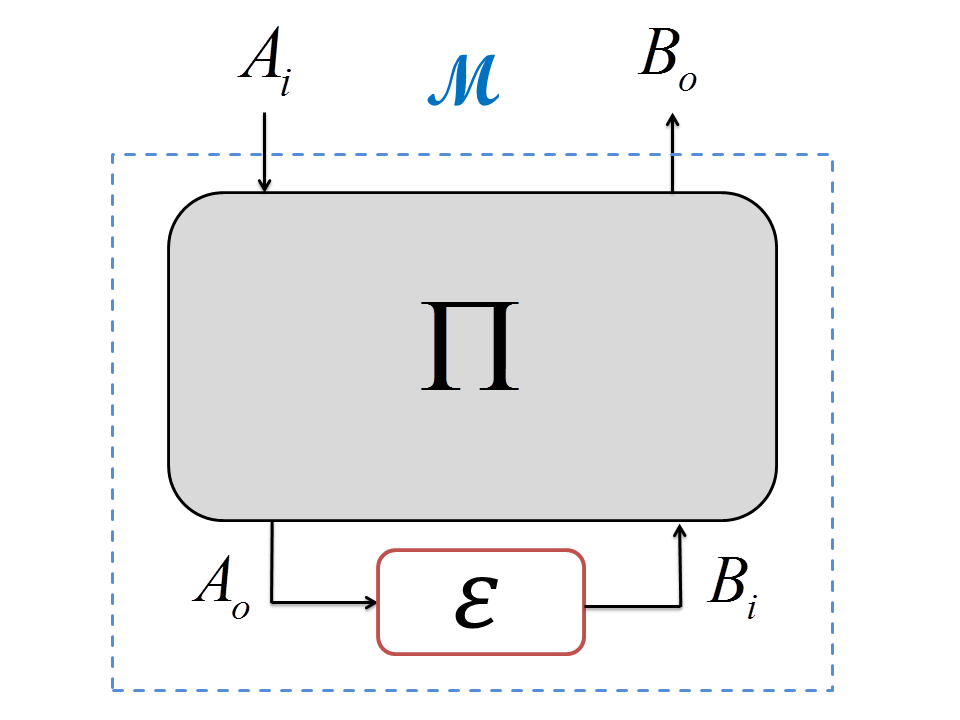
Figure 1: Implementing a channel ${\cal M}$ using another channel ${\cal E}$ with QNSC $\Pi$ between Alice and Bob.

The simulation cost problem concerns how much zero-error communication is required to simulate a noisy channel exactly. Particularly, the one-shot zero-error classical simulation cost of ${\cal N}$ assisted by $\Pi$ is the least noiseless symbols $m$ from $A_{o}$ to $B_{i}$ so that ${\cal M}$ can simulate ${\cal N}$. In [18], the one-shot simulation cost of a quantum channel ${\cal N}$ is given by

$$\Sigma({\cal N})=\min\operatorname{Tr}T_{B},\ {\rm s.t.}\ J_{AB}\leq{\mathds{1}}_{A}\otimes T_{B}.$$ (1)

Its dual SDP is

$$\Sigma({\cal N})=\max\operatorname{Tr}({J_{AB}}{U_{AB}}),\ {\rm s.t.}\ {{U_{AB}}\geq 0,\operatorname{Tr}_{A}{U_{AB}}={{\mathds{1}}_{B}}},$$

where $J_{AB}$ is the Choi-Jamiołkowski matrix of ${\cal N}$. By strong duality, the values of both the primal and the dual SDP coincide. The so-called “non-commutative graph theory” was first suggested in [25] as the non-commutative graph associated with the channel captures the zero-error communication properties, thus playing a similar role to confusability graph. Let ${\cal N}(\rho)=\sum_{k}E_{k}\rho E_{k}^{\dagger}$ be a quantum channel from ${\cal L}(A)$ to ${\cal L}(B)$, where $\sum_{k}E_{k}^{\dagger}E_{k}={\mathds{1}}_{A}$ and $K=K({\cal N})=\operatorname{span}\{E_{k}\}$ denotes the Choi-Kraus operator space of ${\cal N}$. The zero-error classical capacity of a quantum channel in the presence of quantum feedback only depends on the Choi-Kraus operator space of the channel [19]. That is to say, the Choi-Kraus operator space plays a role that is quite similar to the bipartite graph. Such Choi-Kraus operator space $K$ is alternatively called “non-commutative bipartite graph” since it is clear that any classical channel induces a bipartite graph and a confusability graph, while a quantum channel induces a non-commutative bipartite graph together with a non-commutative graph [18].

Back to the simulation cost problem, since there might be more than one channel with Choi-Kraus operator space included in $K$, the exact simulation cost of the “cheapest” one among these channels was defined as the one-shot zero-error classical simulation cost of $K$ [18]: $\Sigma(K)=\min\{\Sigma({\cal N}):{\cal N}\text{ is quantum channel and }K({\cal N})<K\}$, where $K({\cal N})<K$ means that $K({\cal N})$ is a subspace of $K$. Then the one-shot zero-error classical simulation cost of a non-commutative bipartite graph $K$ is given by [18]

$$\begin{split}\Sigma(K)&=\min\operatorname{Tr}T_{B}\ \text{ s.t. }\ 0\leq V_{AB}\leq{\mathds{1}}_{A}\otimes T_{B},\\ &\phantom{=\min\operatorname{Tr}T_{B}\text{ s.t. }}\operatorname{Tr}_{B}V_{AB}={\mathds{1}}_{A},\\ &\phantom{=\min\operatorname{Tr}T_{B}\text{ s.t. }}\operatorname{Tr}({\mathds{1}}-P)_{AB}V_{AB}=0.\end{split}$$ (2)

Its dual SDP is

$$\begin{split}\Sigma(K)&=\max\operatorname{Tr}S_{A}\ \text{ s.t. }\ 0\leq U_{AB},\ \operatorname{Tr}_{A}U_{AB}={\mathds{1}}_{B},\\ &\phantom{=\max\operatorname{Tr}S_{A}\text{ }}P_{AB}(S_{A}\otimes{\mathds{1}}_{B}-U_{AB})P_{AB}\leq 0,\end{split}$$ (3)

where $P_{AB}$ denotes the projection onto the support of the Choi-Jamiołkowski matrix of ${\cal N}$. Then by strong duality, values of both the primal and the dual SDP coincide. It is evident that $\Sigma(K)$ is sub-multiplicative, which means that for two non-commutative bipartite graphs $K_{1}$ and $K_{2}$, $\Sigma({K_{1}}\otimes{K_{2}})\leq\Sigma({K_{1}})\Sigma({K_{2}})$. Furthermore, the multiplicativity of $\Sigma(K)$ for classical-quantum (cq) graphs as well as extremal graphs were known but the general case was left as an open problem [18]. By the regularization, the no-signalling assisted zero-error simulation cost is

$$S_{0,NS}(K)=\inf_{n\geq 1}\frac{1}{n}\log\Sigma\left(K^{\otimes n}\right).$$

As noted in previous work [18, 19],

$$C_{0,NS}(K)\leq C_{\text{minE}}(K)\leq S_{0,NS}(K),$$

where $C_{0,NS}(K)$ is the QSNC assisted classical zero-error capacity and $C_{\text{minE}}(K)$ is the minimum of the entanglement-assisted classical capacity [3, 20] of quantum channels ${\cal N}$ such that $K({\cal N})<K$.

Semidefinite programs [21] can be solved in polynomial time in the program description [22] and there exist several different algorithms employing interior point methods which can compute the optimum value of semidefinite programs efficiently [23, 24]. The CVX software package [28] for MATLAB allows one to solve semidefinite programs efficiently.

In this paper, we focus on the multiplicativity of $\Sigma(K)$ for general non-commutative bipartite graph $K$. We start from the simulation cost of two different graphs and give a sufficient condition which contains all the known multiplicative cases such as cq graphs and extremal graphs. Then we consider about the simulation cost $\Sigma(K)$ when the “cheapest” subspace is full-rank and prove the multiplicativity of one-shot simulation cost in this case. We further explicitly construct a special class of non-commutative bipartite graphs $K_{\alpha}$ whose one-shot simulation cost is non-multiplicative. We also exploit some more properties of $K_{\alpha}$ as well as cheapest-low-rank graphs. Finally, we exhibit a lower bound in order to offer an estimation of the asymptotic simulation cost.

II Main results

II-A A sufficient condition of the multiplicativity of simulation cost

Theorem 1

Let ${K_{1}}$ and ${K_{2}}$ be non-commutative bipartite graphs of two quantum channels ${\cal N}_{1}:{\cal L}(A_{1})\to{\cal L}(B_{1})$ and ${{\cal N}_{2}}:{\cal L}(A_{2})\to{\cal L}(B_{2})$ with support projections $P_{{A_{1}}{B_{1}}}$ and $P_{{A_{2}}{B_{2}}}$, respectively. Suppose the optimal solutions of SDP(3) for $\Sigma({K_{1}})$ and $\Sigma(K_{2})$ are $\left\{{{S_{{A_{1}}}},{U_{1}}}\right\}$ and $\left\{{{S_{{A_{2}}}},{U_{2}}}\right\}$. If at least one of $S_{{A_{1}}}$ and $S_{{A_{2}}}$ satisfy

$${P_{{A_{i}}{B_{i}}}}({S_{{A_{i}}}}\otimes{{\mathds{1}}_{{B_{i}}}}){P_{{A_{i}}{B_{i}}}}\geq 0,i=1~{}\text{or}~{}2,$$ (4)

then

$$\Sigma({K_{1}}\otimes{K_{2}})=\Sigma({K_{1}})\Sigma({K_{2}}).$$

Furthermore,

$$S_{0,NS}(K_{1}\otimes K_{2})=S_{0,NS}(K_{1})+S_{0,NS}(K_{2}).$$

Proof.

It is obvious that ${U_{1}}\otimes{U_{2}}\geq 0\text{ and }\operatorname{Tr}_{{A_{1}}{A_{2}}}({U_{1}}\otimes{U_{2}})={{\mathds{1}}_{{B_{1}}{B_{2}}}}$. For convenience, let $P_{{A_{1}}{B_{1}}}=P_{1}$ and $P_{{A_{2}}{B_{2}}}=P_{2}$. Without loss of generality, we assume that ${P_{2}}({S_{{A_{2}}}}\otimes{{\mathds{1}}_{{B_{2}}}}){P_{2}}\geq 0$. From the last constraint of SDP(2), we have that ${P_{1}}\left({{S_{{A_{1}}}}\otimes{{\mathds{1}}_{{B_{1}}}}}\right){P_{1}}\leq{P_{1}}{U_{1}}{P_{1}}$ and ${P_{2}}({S_{{A_{2}}}}\otimes{{\mathds{1}}_{{B_{2}}}}){P_{2}}\leq{P_{2}}{U_{2}}{P_{2}}$. Note that ${P_{1}}\left({{S_{{A_{1}}}}\otimes{{\mathds{1}}_{{B_{1}}}}}\right){P_{1}}\otimes{P_{2}}({S_{{A_{2}}}}\otimes{{\mathds{1}}_{{B_{2}}}}){P_{2}}\leq{P_{1}}{U_{1}}{P_{1}}\otimes{P_{2}}({S_{{A_{2}}}}\otimes{{\mathds{1}}_{{B_{2}}}}){P_{2}}$. It is easy to see that

$$\begin{split}&{P_{1}}\otimes{P_{2}}\left({{S_{{A_{1}}}}\otimes{S_{{A_{2}}}}\otimes{{\mathds{1}}_{{B_{1}}{B_{2}}}}-{U_{1}}\otimes{U_{2}}}\right){P_{1}}\otimes{P_{2}}\\ \leq&{P_{1}}{U_{1}}{P_{1}}\otimes[{P_{2}}({S_{{A_{2}}}}\otimes{{\mathds{1}}_{{B_{2}}}}){P_{2}}-{P_{2}}{U_{2}}{P_{2}}]\leq 0.\end{split}$$ (5)

Hence, $\left\{{{S_{{A_{1}}}}\otimes{S_{{A_{2}}}},{U_{1}}\otimes{U_{2}}}\right\}$ is a feasible solution of SDP(3) for $\Sigma({K_{1}}\otimes{K_{2}})$, which means that $\Sigma({K_{1}}\otimes{K_{2}})\geq\Sigma({K_{1}})\Sigma({K_{2}})$. Since $\Sigma(K)$ is sub-multiplicative, we can conclude that $\Sigma({K_{1}}\otimes{K_{2}})=\Sigma({K_{1}})\Sigma({K_{2}})$.

Furthermore, for $K_{2}^{\otimes n}$, it is easy to see that $\{S_{A_{2}}^{\otimes n},U_{2}^{\otimes n}\}$ is a feasible solution of SDP(3) for $\Sigma(K_{2}^{\otimes n})$ and ${P_{2}^{\otimes n}}({S_{{A_{2}}}^{\otimes n}}\otimes{{\mathds{1}}_{{B_{2}}}}^{\otimes n}){P_{2}^{\otimes n}}\geq 0$. Therefore, $\Sigma(K_{2}^{\otimes n})=\Sigma(K_{2})^{n}$ and

$$\Sigma[(K_{1}\otimes K_{2})^{\otimes n}]=\Sigma(K_{1}^{\otimes n}\otimes K_{2}^{\otimes n})=\Sigma(K_{1}^{\otimes n})\Sigma(K_{2}^{\otimes n}).$$

Hence,

$$S_{0,NS}(K_{1}\otimes K_{2}) =\inf_{n\geq 1}\frac{1}{n}\log\Sigma\left(K_{1}^{\otimes n}\otimes K_{2}^{\otimes n}\right)$$

$$=\inf_{n\geq 1}\frac{1}{n}\log\Sigma(K_{1}^{\otimes n})\Sigma(K_{2}^{\otimes n})$$

$$=S_{0,NS}(K_{1})+S_{0,NS}(K_{2}).$$

$\sqcap$$\sqcup$

In [26], the activated zero-error no-signalling assisted capacity has been studied. Here, we consider about the corresponding simulation cost problem.

Corollary 2

For any non-commutative bipartite graph K, let $\Delta_{\ell}=\sum_{k=1}^{\ell}|kk\rangle\!\langle kk|$ be the non-commutative bipartite graph of a noiseless channel with $\ell$ symbols, then

$${\Sigma(K\otimes\Delta_{\ell})}={\ell}\Sigma(K),$$

which means that noiseless channel cannot reduce the simulation cost of any other non-commutative bipartite graph.

Proof.

It is evident that $\Delta_{\ell}$ satisfies the condition in Theorem 1. Then, ${\Sigma(K\otimes\Delta_{\ell})}=\ell\Sigma(K)$.     $\sqcap$$\sqcup$

II-B Simulation cost of the cheapest-full-rank non-commutative bipartite graph

Definition 3

Given a non-commutative bipartite graph $K$ with support projection $P_{AB}$. Assume the “cheapest channel” in this space is ${\cal N}_{c}$ with Choi-Jamiołkowski matrix $J_{{\cal N}_{c}}$. $K$ is said to be cheapest-full-rank if there exists ${\cal N}_{c}$ such that $rank(J_{{\cal N}_{c}})=rank(P_{AB})$. Otherwise, $K$ is said to be cheapest-low-rank.

Lemma 4

For a quantum channel ${\cal N}$ with Choi-Jamiołkowski matrix $J_{AB}$ and support projection $P_{AB}$, if $P_{AB}CP_{AB}=P_{AB}DP_{AB}$, then $\operatorname{Tr}(CJ_{AB})=\operatorname{Tr}(DJ_{AB})$.

Proof.

It is easy to see that

$$\operatorname{Tr}(CJ_{AB}) =\operatorname{Tr}(CP_{AB}J_{AB}P_{AB})=\operatorname{Tr}(P_{AB}CP_{AB}J_{AB})$$

$$=\operatorname{Tr}(P_{AB}DP_{AB}J_{AB})=\operatorname{Tr}(DJ_{AB}).$$

$\sqcap$$\sqcup$

Proposition 5

For any non-commutative bipartite graph K with support projection $P_{AB}$, suppose that the cheapest channel is ${\cal N}_{c}$ and the optimal solution of SDP (3) is $\{S_{A},U_{AB}\}$. Assume that

$$P_{AB}(S_{A}\otimes{\mathds{1}}_{B}-U_{AB})P_{AB}=-W_{AB}\text{ and }W_{AB}\geq 0.$$ (6)

Then, we have that

$$\operatorname{Tr}W_{AB}J_{AB}=0,$$ (7)

and $U_{AB}$ is also the optimal solution of $\Sigma({\cal N}_{c})$, where $J_{AB}$ is the Choi-Jamiołkowski matrix of ${\cal N}_{c}$.

Proof.

On one hand, since ${\cal N}_{c}$ is the cheapest channel, $\Sigma(K)$ will equal to $\Sigma({\cal N}_{c})$, also noting that $\{S_{A},U_{AB}\}$ is the optimal solution, we have

$$\begin{split}\operatorname{Tr}{S_{A}}&=\Sigma(K)=\Sigma({\cal N}_{c})\\ &=\max\operatorname{Tr}{J_{AB}}{V_{AB}},\ {\rm s.t.}\ {{V_{AB}}\geq 0,\operatorname{Tr}_{A}{V_{AB}}={{\mathds{1}}_{B}}},\\ &\geq\operatorname{Tr}{J_{AB}}{U_{AB}}.\end{split}$$ (8)

On the other hand, it is evident that $W_{AB}=P_{AB}WP_{AB}$, then $P_{AB}U_{AB}P_{AB}=P_{AB}(W_{AB}+S_{A}\otimes{\mathds{1}}_{B})P_{AB}$. From Lemma 4, we can conclude that $\operatorname{Tr}U_{AB}J_{AB}=\operatorname{Tr}(W_{AB}+S_{A}\otimes{\mathds{1}}_{B})J_{AB}=\operatorname{Tr}W_{AB}J_{AB}+\operatorname{Tr}(S_{A}\otimes{\mathds{1}}_{B})J_{AB}$.

For Choi-Jamiołkowski matrix $J_{AB}$, we have that

$$\begin{split}\operatorname{Tr}({S_{A}}\otimes{{\mathds{1}}_{B}}){J_{AB}}&=\operatorname{Tr}_{A}\operatorname{Tr}_{B}[({S_{A}}\otimes{{\mathds{1}}_{B}}){J_{AB}}]\\ &=\operatorname{Tr}_{A}[{S_{A}}(\operatorname{Tr}_{B}{J_{AB}})]=\operatorname{Tr}{S_{A}},\end{split}$$ (9)

then

$$\operatorname{Tr}U_{AB}J_{AB}=\operatorname{Tr}W_{AB}J_{AB}+\operatorname{Tr}{S_{A}}.$$ (10)

Combining (8) and (10), and noting that $W_{AB},J_{AB}\geq 0$, we can conclude that $\operatorname{Tr}W_{AB}J_{AB}=0$ and $U_{AB}$ is also the optimal solution of $\Sigma({\cal N}_{c})$.     $\sqcap$$\sqcup$

Theorem 6

For any cheapest-full-rank non-commutative bipartite graph $K$, we have

$$\begin{split}\Sigma(K)&=\max\operatorname{Tr}S_{A}\ \text{ s.t. }\ 0\leq U_{AB},\ \operatorname{Tr}_{A}U_{AB}={\mathds{1}}_{B},\\ &\phantom{=\max\operatorname{Tr}S_{A}\text{ s.t. }}P_{AB}(S_{A}\otimes{\mathds{1}}_{B}-U_{AB})P_{AB}=0.\end{split}$$ (11)

Also, $\Sigma({K}\otimes{K})=\Sigma({K})\Sigma({K})$. Consequently, $S_{0,NS}(K)=\log\Sigma(K)$.

And for any other non-commutative bipartite graph $K^{\prime}$, $S_{0,NS}(K\otimes K^{\prime})=S_{0,{\text{NS}}}(K)+S_{0,NS}(K^{\prime})$.

Proof.

We first assume that $W\neq 0$. Notice $rank(J_{AB})=rank(P_{AB})$, it is easy to see that $\operatorname{Tr}WJ_{AB}>0$, which contradicts Eq. (7). Hence the assumption is false, and we can conclude that $P_{AB}(S_{A}\otimes{\mathds{1}}_{B}-U_{AB})P_{AB}=0$.

Then by Theorem 1, it is easy to see that $\Sigma(K\otimes K)=\Sigma(K)\Sigma(K)$. Therefore,

$$S_{0,{\text{NS}}}(K)=\inf_{n\geq 1}\frac{1}{n}\log\Sigma(K^{\otimes n})=\log\Sigma(K).$$

Furthermore, for any other non-commutative bipartite graph $K^{\prime}$, $S_{0,NS}(K\otimes K^{\prime})=S_{0,{\text{NS}}}(K)+S_{0,NS}(K^{\prime})$.     $\sqcap$$\sqcup$

Noting that any rank-2 Choi-Kraus operator space is always cheapest-full-rank, we have the following immediate corollary.

Corollary 7

For any rank-2 Choi-Kraus operator space $K$, $S_{0,NS}(K)=\log\Sigma(K)$. And for any other non-commutative bipartite graph $K^{\prime}$, $S_{0,NS}(K\otimes K^{\prime})=S_{0,NS}(K)+S_{0,NS}(K^{\prime})$.

II-C The one-shot simulation cost is not multiplicative

We will focus on the non-commutative bipartite graph $K_{\alpha}$ with support projection $P_{AB}=\sum\limits_{j=0}^{2}|\psi_{j}\rangle\!\langle\psi_{j}|$, where $|\psi_{0}\rangle=\frac{1}{\sqrt{3}}(|00\rangle+|01\rangle+|12\rangle),|\psi_{1}\rangle=\cos\alpha|02\rangle+\sin\alpha|11\rangle,|\psi_{2}\rangle=|10\rangle$.

To prove that $K_{\alpha}$ ($0<\cos^{2}\alpha<1$) is feasible to be a class of feasible non-commutative bipartite graphs, we only need to find a channel ${\cal N}$ with Choi-Jamiołkowski matrix $J_{AB}$ such that $P_{AB}J_{AB}=J_{AB}$ and $\text{rank}(P_{AB})=\text{rank}(J_{AB})$ . Assume that $J_{AB}=\sum\limits_{j=0}^{2}a_{j}|\psi_{j}\rangle\!\langle\psi_{j}|$, then it is equivalent to prove that $\operatorname{Tr}_{B}J_{AB}={\mathds{1}}_{A}$ and $J_{AB}\geq 0$ has a feasible solution. Therefore,

$$\frac{2}{3}a_{0}+\cos^{2}\alpha a_{1}=1,a_{0}+a_{1}+a_{2}=2,a_{0},a_{1},a_{2}>0.$$

Noting that when we choose $0<a_{1}<\frac{1}{2}$, $a_{0}=\frac{3}{2}(1-\cos^{2}\alpha a_{1})$ and $a_{2}=\frac{1-(2-3\cos^{2}\alpha)a_{1}}{2}$ will be positive, which means that there exists such $J_{AB}$. Hence, $K_{\alpha}$ is a feasible noncommutative bipartite graph.

Theorem 8

There exists non-commutative bipartite graph K such that $\Sigma(K\otimes K)<\Sigma(K)^{2}$.

Proof.

As we have shown above, it is reasonable to focus on $K_{\alpha}$. Then, by semidefinite programming assisted with useful tools CVX [28] and QETLAB [29], the gap between one-shot and two-shot average no-signalling assisted zero-error simulation cost of $K_{\alpha}(0.25\leq\cos^{2}\alpha\leq 0.35)$ is presented in Figure 2.

To be specfic, when $\alpha=\pi/3$, it is clear that $\cos^{2}\alpha=1/4$ and $|\psi_{1}\rangle=\frac{1}{2}|02\rangle+\frac{\sqrt{3}}{2}|11\rangle$. Assume that $S=3.1102|0\rangle\!\langle 0|-0.5386|1\rangle\!\langle 1|$ and $U=\frac{99}{50}|u_{1}\rangle\!\langle u_{1}|+\frac{51}{50}|u_{2}\rangle\!\langle u_{2}|$, where $|u_{1}\rangle=\frac{10}{3\sqrt{33}}|00\rangle+\frac{5}{3}\sqrt{\frac{2}{33}}|01\rangle+\frac{7}{3\sqrt{11}}|12\rangle$ and $|u_{2}\rangle=\frac{1}{\sqrt{51}}|02\rangle-\frac{5}{3}\sqrt{\frac{2}{17}}|10\rangle+\frac{10}{3\sqrt{17}}|11\rangle$, and it can be checked that $U\geq 0$, $\operatorname{Tr}_{A}U={\mathds{1}}_{B}$ and $P_{AB}(S_{A}\otimes{\mathds{1}}_{B}-U_{AB})P_{AB}\leq 0$. Then $\{S,U\}$ is a feasible solution of SDP (3) for $\Sigma(K_{\pi/3})$, which means that $\Sigma(K_{\pi/3})\geq\operatorname{Tr}S=2.5716$. Similarily, we can find a feasible solution of SDP (2) for $\Sigma(K_{\pi/3}\otimes K_{\pi/3})$ through Matlab such that $\Sigma(K_{\pi/3}\otimes K_{\pi/3})^{1/2}\leq 2.57$. (The code is available at [27].) Hence, there is a non-vanishing gap between $\Sigma(K_{\pi/3})$ and $\Sigma(K_{\pi/3}\otimes K_{\pi/3})^{1/2}$.     $\sqcap$$\sqcup$

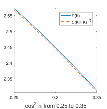
Figure 2: The one-shot (red) and two-shot average (blue) no-signalling assisted zero-error simulation cost of $K_{\alpha}$ over the parameter $\alpha$.

We have shown that one-shot simulation cost of cheapest-full-rank non-commutative bipartite graphs is multiplicative while there are counterexamples for cheapest-low-rank ones. However, not all cheapest-low-rank graphs have non-multiplicative simulation cost. Here is one trivial counterexample. Let $K=\text{span}\{|0\rangle\langle 0|,|1\rangle\langle 0|,|1\rangle\langle 1|\}$, the cheapest channel is a constant channel ${\cal N}$ with $E_{0}=|1\rangle\langle 0|$ and $E_{1}=|1\rangle\langle 1|$. In this case, $\Sigma(K\otimes K)=\Sigma(K)\Sigma(K)=1.$ Actually, the simulation cost problem of cheapest-low-rank non-commutative bipartite graphs is complex since it is hard to determine the cheapest subspace under tensor powers. Therefore, it is difficult to calculate the asymptotic simulation cost of non-multiplicative cases.

In [19], $K$ is called non-trivial if there is no constant channel ${\cal N}_{0}:\rho\to|\beta\rangle\!\langle\beta|$ with $K({\cal N}_{0})<K$, where $|\beta\rangle$ is a state vector. It was known that $K$ is non-trivial if and only if the no-signalling assisted zero-error capacity is positive, say $C_{0,NS}(K)>0$. Clearly we have the following result.

Proposition 9

For any non-commutative bipartite graph $K$, $S_{0,NS}(K)>0$ if and only if $K$ is non-trivial.

Proof.

If $K$ is non-trivial, it is obvious that $S_{0,NS}(K)\geq C_{0,NS}(K)>0$. Otherwise, $0\leq S_{0,NS}(K)\leq S_{0,NS}({\cal N}_{0})=0$, which means that $S_{0,NS}(K)=0$.     $\sqcap$$\sqcup$

II-D A lower bound

Let us introduce a revised SDP which has the same simplified form in cq-channel case:

$$\begin{split}\Sigma^{-}(K)&=\max\operatorname{Tr}S_{A}\ \text{ s.t. }\ S_{A}\geq 0,U_{AB}\geq 0\ \operatorname{Tr}_{A}U_{AB}={\mathds{1}}_{B},\\ &\phantom{=\max\operatorname{Tr}S_{A}\text{ s.t. }}P_{AB}(S_{A}\otimes{\mathds{1}}_{B}-U_{AB})P_{AB}\leq 0,\end{split}$$ (12)

Lemma 10

For any non-commutative bipartite graphs $K_{1}$ and $K_{2}$,

$$\Sigma^{-}(K_{1}\otimes K_{2})\geq\Sigma^{-}(K_{1})\Sigma^{-}(K_{2}).$$

Consequently, $\Sigma^{-}({K_{1}})\Sigma^{-}({K_{2}})\leq\Sigma({K_{1}}\otimes{K_{2}})\leq\Sigma({K_{1}})\Sigma({K_{2}})$.

Proof.

From SDP (12), noting that $P_{AB}(S_{A}\otimes{\mathds{1}}_{B})P_{AB}\geq 0$, it is easy to prove $\Sigma^{-}(K_{1}\otimes K_{2})\geq\Sigma^{-}(K_{1})\Sigma^{-}(K_{2})$ by similar technique applied in Theorem 3. Therefore, $\Sigma^{-}({K_{1}})\Sigma^{-}({K_{2}})\leq\Sigma^{-}({K_{1}}\otimes{K_{2}})\leq\Sigma({K_{1}}\otimes{K_{2}})\leq\Sigma({K_{1}})\Sigma({K_{2}})$.     $\sqcap$$\sqcup$

Proposition 11

For a general non-commutative bipartite graph $K$,

$$\log{\Sigma^{-}}(K)\leq{S_{0,NS}}(K)\leq\log\Sigma(K).$$

Proof.

By Lemma 10, it is easy to see that ${\Sigma^{-}}{(K)^{n}}\leq\Sigma(K^{\otimes n})\leq\Sigma{(K)^{n}}$. Then, $\log{\Sigma^{-}}(K)\leq{S_{0,NS}}(K)\leq\log\Sigma(K)$. Also, it is obvious that ${S_{0,NS}}(K)$ will equal to $\log\Sigma(K)$ when $\Sigma^{-}(K)=\Sigma(K).$     $\sqcap$$\sqcup$

III Conclusions

In sum, for two different non-commutative bipartite graphs, we give sufficient conditions for the multiplicativity of one-shot simulation cost as well as the additivity of the asymptotic simulation cost. The case of cheapest-full-rank non-commutative bipartite graphs has been completely solved while the cheapest-low-rank graphs have a more complex structure. We further show that the one-shot no-signalling assisted classical zero-error simulation cost of non-commutative bipartite graphs is not multiplicative. We provide a lower bound of $\Sigma(K)$ such that the asymptotic zero-error simulation cost can be estimated by $\log\Sigma^{-}(K)\leq S_{0,NS}(K)\leq\log\Sigma(K)$.

It is of great interest to know whether the sufficient condition of multiplicativity in Theorem 1 is also necessary. It also remains unknown about the additivity of the asymptotic simulation cost of general non-commutative bipartite graphs and whether it equals to $\log\Sigma^{-}(K)$.

References

• [1] D. Kretschmann and R. F. Werner, “Tema con variazioni: quantum channel capacity”, New Journal of Physics, vol. 6, no. 1, pp. 26, 2004.
• [2] C. E. Shannon, “A mathematical theory of communication”, Bell System Tech. J, vol. 27, pp. 379-423, 1948.
• [3] C. H. Bennett, P. W. Shor, J. A. Smolin and A. V. Thapliyal, “Entanglement-assisted capacity of a quantum channel and the reverse Shannon theorem”, IEEE Transactions on Information Theory, vol. 48, no. 10, pp. 2637-2655, 2002.
• [4] C. H. Bennett, I. Devetak, A. W. Harrow, P. W. Shor and A. Winter, “The Quantum Reverse Shannon Theorem and Resource Tradeoffs for Simulating Quantum Channels”, IEEE Transactions on Information Theory, vol. 60, no. 3, pp. 2926-2959, 2014.
• [5] M. Berta, M. Christandl and R. Renner, “The Quantum Reverse Shannon Theorem Based on One-Shot Information Theory”, Communications in Mathematical Physics, vol. 306, no.3, pp. 579-615, 2011.
• [6] C. E. Shannon, “The zero-error capacity of a noisy channel”, IRE Transactions on Information Theory, vol. 2, no. 3, pp. 8-19, 1956.
• [7] T. S. Cubitt, D. Leung, W. Matthews, and A. Winter, “Improving zero-error classical communication with entanglement”, Physical Review Letters, vol. 104, no. 23, pp. 230503, 2010.
• [8] D. Leung, L. Mančinska, W. Matthews, M. Ozols and A. Roy, “Entanglement can increase asymptotic rates of zero-error classical communication over classical channels”, Communications in Mathematical Physics, vol. 311, pp. 97-111, 2012.
• [9] R. Duan, “Super-activation of zero-error capacity of noisy quantum channels”, arXiv:0906.2526.
• [10] R. Duan and Y. Shi, “Entanglement between two uses of a noisy multipartite quantum channel enables perfect transmission of classical information”, Physical Review Letters, vol. 101, no. 02, pp. 020501, 2008.
• [11] T. S. Cubitt, J. Chen and A. W. Harrow, “Superactivation of the asymptotic zero-error classical capacity of a quantum channel”, IEEE Transactions on Information Theory, vol. 57, no. 12, pp. 8114-8126, 2011.
• [12] T. S. Cubitt and G. Smith, “An extreme form of super-activation for quantum zero-error capacities”, IEEE Transactions on Information Theory, vol. 58, no. 3, pp. 1953-1961, 2012.
• [13] D. Beckman, D. Gottesman, M. A. Nielsen and J. Preskill, “Causal and localizable quantum operations”, Physical Review A, vol. 64, no. 05, pp. 052309, 2001.
• [14] T. Eggeling, D. Schlingemann and R. F. Werner, “Semicausal operations are semilocalizable”, Europhysics Letters, vol. 57, no. 6, pp. 782-788, 2002.
• [15] M. Piani, M. Horodecki, P. Horodecki and R. Horodecki, “Properties of quantum nonsignaling boxes”, Physical Review A, vol. 74, no. 01, pp. 012305, 2006.
• [16] O. Oreshkov, F. Costa, and Č. Brukner, “Quantum correlations with no causal order”, Nature communications, vol. 3, no. 10, pp. 1092, 2012.
• [17] T. S. Cubitt, D. Leung, W. Matthews, and A. Winter, “Zero-error channel capacity and simulation assisted by non-local correlations”, IEEE Transactions on Information Theory, vol. 57, no. 8, pp. 5509-5523, 2011.
• [18] R. Duan and A. Winter, “Non-Signalling Assisted Zero-Error Capacity of Quantum Channels and an Information Theoretic Interpretation of the Lovász Number”, IEEE Transactions on Information Theory, vol. 62, no. 2, pp. 891–914, 2016.
• [19] R. Duan, S. Severini and A. Winter, “On zero-error communication via quantum channels in the presence of noiseless feedback”, arXiv:1502.02987.
• [20] C. H. Bennett, P. W. Shor, J. A. Smolin, and A. V Thapliyal, “Entanglement-assisted classical capacity of noisy quantum channels,” Physical Review Letters, vol. 83, no. 15, pp. 3081 (1999).
• [21] L. Vandenberghe, S. Boyd, “Semidefinite Programming”, SIAM Review, vol. 38, no. 1, pp. 49-95, 1996.
• [22] L. G. Khachiyan, “Polynomial algorithms in linear programming”, USSR Computational Mathematics and Mathematical Physics, vol. 20, no. 1, pp. 53–72, 1980.
• [23] F. Alizadeh, “Interior point methods in semidefinite programming with applications to combinatorial optimization”, SIAM Journal on Optimization, vol. 5, no. 1, pp. 13–51, 1995.
• [24] E. De Klerk, “Aspects of semidefinite programming: interior point algorithms and selected applications”, Springer Science & Business Media, 2002.
• [25] R. Duan, S. Severini, and A. Winter, “Zero-error communication via quantum channels, non-commutative graphs and a quantum Lovász number”, IEEE Transactions on Information Theory, vol. 59, no. 2, pp. 1164-1174, 2013.
• [26] R. Duan and X. Wang, Activated zero-error classical capacity of quantum channels in the presence of quantum no-signalling correlations, arXiv:1505.00907.
• [27] X. Wang, Supplementary software for implementing the one-shot QSNC assisted zero-error simulation cost is not multiplicative, https://github.com/xinwang1/QSNC-simulation-cost.
• [28] M. Grant and S. Boyd. CVX: Matlab software for disciplined convex programming, version 2.1. http://cvxr.com/cvx, 2014.
• [29] N. Johnston, A. Cosentino, and V. Russo. QETLAB: A MATLAB toolbox for quantum entanglement, http://qetlab.com, 2015.