Cosmology in new gravitational scalar-tensor theories

Abstract

We investigate the cosmological applications of new gravitational scalar-tensor theories, which are novel modifications of gravity possessing $2+2$ propagating degrees of freedom, arising from a Lagrangian that includes the Ricci scalar and its first and second derivatives. Extracting the field equations we obtain an effective dark energy sector that consists of both extra scalar degrees of freedom, and we determine various observables. We analyze two specific models and we obtain a cosmological behavior in agreement with observations, i.e. transition from matter to dark energy era, with the onset of cosmic acceleration. Additionally, for a particular range of the model parameters, the equation-of-state parameter of the effective dark energy sector can exhibit the phantom-divide crossing. These features reveal the capabilities of these theories, since they arise solely from the novel, higher-derivative terms.

I Introduction

According to the standard model of cosmology, which is supported by a huge amount of observations, the expansion of the universe includes two accelerated phases, at early and late times respectively. Since this behavior cannot be described within the standard paradigm of physics, namely within general relativity and Standard Model of particles, physicists try to increase the degrees of freedom of the theory. In principle there are two ways to achieve it. The first is to modify the universe content by introducing new, exotic, fields, such as the inflaton Olive:1989nu ; Bartolo:2004if or the concept of dark energy Copeland:2006wr ; Cai:2009zp . The second is to consider that the extra degrees of freedom are gravitationally oriented, i.e. that they arise from a gravitational modification at specific scales Nojiri:2006ri ; Capozziello:2011et . Note that the second approach, apart from the above cosmological motivation, has a theoretical motivation too, namely to improve the UltraViolet behavior of gravity Stelle:1976gc ; Biswas:2011ar . Finally, we mention that the above constructions are not separated by strict boundaries, since one can completely or partially transform between them, or build theories where both extensions are used.

In order to construct a gravitational modification one can add higher-order corrections to the action of general relativity, as in $f(R)$ gravity Sotiriou:2008rp ; DeFelice:2010aj ; Nojiri:2010wj ; Nojiri:2006gh , in Gauss-Bonnet and $f(G)$ gravity Nojiri:2005jg ; DeFelice:2008wz , in Lovelock gravity Lovelock:1971yv ; Deruelle:1989fj , in Weyl gravity Mannheim:1988dj ; Flanagan:2006ra , etc. However, one should ensure himself that the additional degrees of freedom introduced in such modifications do not present a ghost behavior or other kind of catastrophic instabilities, at the background or perturbation levels. Indeed, Horndeski was able to construct the most general single-scalar field theory with second-order equations of motion and thus without ghosts in Horndeski:1974wa , a construction which was re-discovered in the framework of Galileon modifications in Nicolis:2008in ; Deffayet:2009wt ; Deffayet:2009mn ; Deffayet:2011gz . These classes of theories involve $2+1$ propagating degrees of freedom, that is one extra comparing to general relativity (see also the extension to beyond Horndeski theories, with still one extra propagating degree of freedom Zumalacarregui:2013pma ; Gleyzes:2014dya ; Gao:2014soa ; Gleyzes:2014qga ; Gao:2014fra ).

Hence, a question arises naturally: can we construct gravitational modifications beyond the above classes, i.e. possessing for instance $2+2$ propagating degrees of freedom, while still being ghost-free? Indeed, such a multi-scalar modification was developed in Padilla:2010de ; Padilla:2012dx , and it was shown to be the most general multi-scalar tensor theory in a flat background Sivanesan:2013tba but not in a general one Kobayashi:2013ina . Nevertheless, the construction of the most general field equations for a bi-scalar Ohashi:2015fma or multi-scalar theory still attracts a lot of interest in the literature Padilla:2013jza , as well as the corresponding cosmological and black-hole applications Padilla:2010tj ; Charmousis:2014zaa .

However, although the construction of ghost-free theories with $2+2$ or more propagating degrees of freedom is obtained relatively easily in the scalar-field language, it proves to be a harder task if one starts from the pure gravitational modification formulation. Indeed, in Naruko:2015zze the authors managed to construct a modified gravity using the Ricci scalar and its first and second derivatives, which under a specific Lagrangian choice is free of ghosts, possessing $2+2$ degrees of freedom, namely 2 scalar degrees and 2 tensor ones. These constructions, named gravitational scalar-tensor theories, are equivalent with specific cases of generalized bi-Galileon theories, however whether there is a complete one-to-one correspondence between them is an open question.

In the present work we are interested in investigating the cosmological behavior in gravitational scalar-tensor theories. In particular, we desire to study the late-time evolution of a universe governed by such a gravitational modification, and examine whether we can obtain acceleration without the use of an explicit cosmological constant, namely arising solely from the novel terms of the theory. The plan of the work is as follows: In Section II we present the new gravitational scalar-tensor theories and we derive the corresponding field equations in a general background. Then, in Section III we apply them in a cosmological framework, and we explicitly investigate two specific models. Finally, Section IV is devoted to summary and discussion.

II New gravitational scalar-tensor theories

In this section we briefly review the construction of gravitational scalar-tensor theories following Naruko:2015zze , starting from the modified gravitational action and resulting in the corresponding specific bi-scalar action. Then we derive the general equations of motion for both metric and scalar degrees of freedom, in a general background.

The starting point for the construction of new gravitational scalar-tensor theories is the idea to (re-)formulate generalized scalar-tensor theories only in terms of the metric and its derivatives, without the use of a scalar field Naruko:2015zze . Hence, one starts by extending the $f(R)$ action to include derivatives of the Ricci scalar, namely

$$S=\int d^{4}\sqrt{-g}\,f\left(R,(\nabla R)^{2},\square R\right),$$ (1)

where $(\nabla R)^{2}=g^{\mu\nu}\nabla_{\mu}R\nabla_{\nu}R$. These actions, despite their higher derivative nature, using double Lagrange multipliers can be transformed to actions of multi-scalar fields coupled minimally to gravity. A crucial step is the dependence of $f$ on $\square R=\beta$. In the case where it does not enter linearly, namely if $f_{\beta\beta}\neq 0$, where subscripts denote partial derivatives, then (1) can be re-written in the following form:

$$\!\!\!\!\!\!\!\!S=\!\int\!d^{4}x\sqrt{-\hat{g}}\left\{\frac{1}{2}\hat{R}-\frac{1}{2}\hat{g}^{\mu\nu}\left(\partial_{\mu}\chi\partial_{\nu}\chi+e^{-\sqrt{\frac{2}{3}}\chi}\partial_{\mu}\phi\partial_{\nu}\phi\right)\right.$$

$$\left.-\frac{1}{4}\!\left[e^{-\sqrt{\frac{2}{3}}\chi}\phi+e^{-2\sqrt{\frac{2}{3}}\chi}\left(\varphi\,\beta(\phi,(\hat{\nabla}\phi)^{2},\varphi)\!-\!f\right)\right]\!\right\}\!,$$ (2)

where $\chi,\phi$ are scalar fields and $\varphi\equiv f_{\beta}$ (for simplicity, here and in the following, we set the gravitational constant to one). In the above expression the $hat$ denotes a frame conformally related to the original one through $g_{\mu\nu}=\frac{1}{2}e^{-\sqrt{\frac{2}{3}}\chi}\hat{g}_{\mu\nu}$.

If on the other hand $\beta$ does enter linearly, namely if $f_{\beta\beta}=0$, then the function $f$ can be re-written as

$$f(R,(\nabla R)^{2},\square R)=\mathcal{K}((R,(\nabla R)^{2})+\mathcal{G}(R,(\nabla R)^{2})\square R.$$ (3)

If $\mathcal{G}$ depends only on $R$, then through integration by parts the second term of the above relation can be redefined in terms of the first one, and thus this case is equivalent to the $\mathcal{G}=0$ one. However, in the general case where $\mathcal{G}=\mathcal{G}(R,(\nabla R)^{2})$ the above new gravitational scalar-tensor theory can be transformed to the following bi-scalar construction Naruko:2015zze :

$$\!\!\!\!\!\!\!\!\!\!\!\!\!\!\!S=\int d^{4}x\sqrt{-\hat{g}}\left[\frac{1}{2}\hat{R}-\frac{1}{2}\hat{g}^{\mu\nu}\nabla_{\mu}\chi\nabla_{\nu}\chi\right.$$

$$\ \ \ \ \ \ \ \ \ \ \ \ -\frac{1}{\sqrt{6}}e^{-\sqrt{\frac{2}{3}}\chi}\hat{g}^{\mu\nu}\mathcal{G}\nabla_{\mu}\chi\nabla_{\nu}\phi+\frac{1}{4}e^{-2\sqrt{\frac{2}{3}}\chi}\mathcal{K}$$

$$\ \ \ \ \ \ \ \ \ \ \ \ \left.+\frac{1}{2}e^{-\sqrt{\frac{2}{3}}\chi}\mathcal{G}\hat{\square}\phi-\frac{1}{4}e^{-\sqrt{\frac{2}{3}}\chi}\phi\right],$$ (4)

where now

$$\mathcal{K}=\mathcal{K}(\phi,B),\quad\mathcal{G}=\mathcal{G}(\phi,B),$$ (5)

with

$$B=2e^{\sqrt{\frac{2}{3}}\chi}g^{\mu\nu}\nabla_{\mu}\phi\nabla_{\nu}\phi.$$ (6)

The above action contains two scalar fields, namely $\chi$ and $\phi$, however it does so in the specific and suitable combination in order to be equivalent with the original higher-derivative gravitational action. Hence, although in simple $f(R)$ theories the conformal transformation leads to the replacement of the functional degree of freedom of $f(R)$ by a scalar field, in the above constructions the derivatives of $R$ are not replaced by derivatives of the scalar-field in a naive way, but only through the above two-field combination. That is why the authors of Naruko:2015zze named these theories as “new gravitational scalar-tensor theories”, in a sense that they can be understood as the pure gravitational formulations of standard multi-scalar-tensor theories constructed from scalar fields and the metric. Such theories have not been previously investigated and thus they may open new paths towards the construction of gravitational modifications.

In the following we will work with the Einstein-frame version of the above theories, namely with action (II), and thus for simplicity we drop the hats. Varying (II) with respect to the metric leads to the metric field equations

$$\mathcal{E}_{\mu\nu} \!\!=\!\! \frac{1}{2}G_{\mu\nu}+\frac{1}{4}g_{\mu\nu}g^{\alpha\beta}\nabla_{\alpha}\chi\nabla_{\beta}\chi-\frac{1}{2}\nabla_{\mu}\chi\nabla_{\nu}\chi$$ (7)

$$+\frac{1}{4}g_{\mu\nu}\sqrt{\frac{2}{3}}e^{-\sqrt{\frac{2}{3}}\chi}g^{\alpha\beta}\mathcal{G}\nabla_{\alpha}\chi\nabla_{\beta}\phi$$

$$-\frac{1}{2}\sqrt{\frac{2}{3}}e^{-\sqrt{\frac{2}{3}}\chi}\mathcal{G}\nabla_{(\mu}\chi\nabla_{\nu)}\phi$$

$$-\sqrt{\frac{2}{3}}g^{\alpha\beta}\nabla_{\alpha}\chi\nabla_{\beta}\phi\,\mathcal{G}_{B}\nabla_{\mu}\phi\nabla_{\nu}\phi$$

$$-\frac{1}{4}g_{\mu\nu}e^{-\sqrt{\frac{2}{3}}\chi}\mathcal{G}\square\phi+\mathcal{G}_{B}(\square\phi)\nabla_{\mu}\phi\nabla_{\nu}\phi$$

$$+\frac{1}{2}e^{-\sqrt{\frac{2}{3}}\chi}\mathcal{G}\nabla_{\mu}\nabla_{\nu}\phi-\frac{1}{2}\nabla_{\kappa}\left(e^{-\sqrt{\frac{2}{3}}\chi}\mathcal{G}\delta^{\lambda}_{(\mu}\delta^{\kappa}_{\nu)}\nabla_{\lambda}\phi\right)$$

$$+\frac{1}{4}\nabla_{\kappa}\left(e^{-\sqrt{\frac{2}{3}}\chi}\mathcal{G}g_{\mu\nu}\nabla^{\kappa}\phi\right)-\frac{1}{8}g_{\mu\nu}e^{-2\sqrt{\frac{2}{3}}\chi}\mathcal{K}$$

$$+\frac{1}{2}e^{-\sqrt{\frac{2}{3}}\chi}\mathcal{K}_{B}\nabla_{\mu}\phi\nabla_{\nu}\phi+\frac{1}{8}g_{\mu\nu}e^{-\sqrt{\frac{2}{3}}\chi}\phi=0,$$

where the parentheses in space-time indices mark symmetrization, and the subscripts in $\mathcal{G}$ and $\mathcal{K}$ denote partial derivatives with respect to the corresponding argument (for instance $\mathcal{G}_{B}=\frac{\partial\mathcal{G}(\phi,B)}{\partial B}$ etc). Similarly, variation of (II) with respect to the scalar fields $\chi$ and $\phi$ leads respectively to their equations of motion, namely

$$\mathcal{E}_{\chi} \!\!=\!\! \square\chi+\frac{1}{3}e^{-\sqrt{\frac{2}{3}}\chi}g^{\mu\nu}\mathcal{G}\nabla_{\mu}\chi\nabla_{\nu}\phi$$ (8)

$$-\frac{2}{3}g^{\mu\nu}\nabla_{\mu}\chi\nabla_{\nu}\phi\,\mathcal{G}_{B}g^{\alpha\beta}\nabla_{\alpha}\phi\nabla_{\beta}\phi$$

$$+\frac{1}{2}\sqrt{\frac{2}{3}}\nabla_{\mu}\left(e^{-\sqrt{\frac{2}{3}}\chi}g^{\mu\nu}\mathcal{G}\nabla_{\nu}\phi\right)$$

$$-\frac{1}{2}\sqrt{\frac{2}{3}}e^{-\sqrt{\frac{2}{3}}\chi}\mathcal{G}\square\phi+\sqrt{\frac{2}{3}}\mathcal{G}_{B}\nabla_{\mu}\phi\nabla_{\nu}\phi\,g^{\mu\nu}\square\phi$$

$$-\frac{1}{2}\sqrt{\frac{2}{3}}e^{-2\sqrt{\frac{2}{3}}\chi}\mathcal{K}+\frac{1}{2}e^{-\sqrt{\frac{2}{3}}\chi}\mathcal{K}_{B}\sqrt{\frac{2}{3}}g^{\mu\nu}\nabla_{\mu}\phi\nabla_{\nu}\phi$$

$$+\frac{1}{4}\sqrt{\frac{2}{3}}e^{-\sqrt{\frac{2}{3}}\chi}\phi=0,$$

and

$$\mathcal{E}_{\phi} \!\!=\!\! -\frac{1}{2}\sqrt{\frac{2}{3}}e^{-\sqrt{\frac{2}{3}}\chi}g^{\mu\nu}\mathcal{G}_{\phi}\nabla_{\mu}\chi\nabla_{\nu}\phi$$ (9)

$$+2\sqrt{\frac{2}{3}}\nabla_{\beta}\left(g^{\mu\nu}\mathcal{G}_{B}g^{\alpha\beta}\nabla_{\alpha}\phi\nabla_{\mu}\chi\nabla_{\nu}\phi\right)$$

$$+\frac{1}{2}\sqrt{\frac{2}{3}}\nabla_{\nu}\left(e^{-\sqrt{\frac{2}{3}}\chi}g^{\mu\nu}\mathcal{G}\nabla_{\mu}\chi\right)$$

$$+\frac{1}{2}e^{-\sqrt{\frac{2}{3}}\chi}\mathcal{G}_{\phi}\square\phi-2\mathcal{G}_{B}(\square\phi)^{2}-2\nabla_{\nu}\mathcal{G}_{B}\square\phi\nabla^{\nu}\phi$$

$$-\frac{1}{2}\sqrt{\frac{2}{3}}\nabla^{\mu}\left(e^{-\sqrt{\frac{2}{3}}\chi}\nabla_{\mu}\chi\,\mathcal{G}\right)+\frac{1}{2}\nabla^{\mu}\left(e^{-\sqrt{\frac{2}{3}}\chi}\,\mathcal{G}_{\phi}\nabla_{\mu}\phi\right)$$

$$-\frac{1}{2}\sqrt{\frac{2}{3}}e^{-\sqrt{\frac{2}{3}}\chi}\nabla^{\mu}\chi\mathcal{G}_{B}\nabla_{\mu}B+\frac{1}{2}e^{-\sqrt{\frac{2}{3}}\chi}\nabla^{\mu}\mathcal{G}_{B}\nabla_{\mu}B$$

$$+\sqrt{\frac{2}{3}}e^{-\sqrt{\frac{2}{3}}\chi}\mathcal{G}_{B}\nabla^{\mu}\left(e^{\sqrt{\frac{2}{3}}\chi}\nabla_{\mu}\chi\nabla^{\nu}\phi\nabla_{\nu}\phi\right)$$

$$+2e^{-\sqrt{\frac{2}{3}}\chi}\mathcal{G}_{B}\nabla^{\mu}\left(e^{\sqrt{\frac{2}{3}}\chi}\nabla^{\nu}\phi\right)\nabla_{\mu}\nabla_{\nu}\phi$$

$$+2\mathcal{G}_{B}R^{\mu\nu}\nabla_{\mu}\phi\nabla_{\nu}\phi+\frac{1}{4}e^{-2\sqrt{\frac{2}{3}}\chi}\mathcal{K}_{\phi}$$

$$-\nabla_{\nu}\left(e^{-\sqrt{\frac{2}{3}}\chi}\mathcal{K}_{B}g^{\mu\nu}\nabla_{\mu}\phi\right)-\frac{1}{4}e^{-\sqrt{\frac{2}{3}}\chi}=0.$$

We stress here that despite the fact that the higher-order term in the action (II) naively seems to be problematic, in the sense that it could lead to higher-order derivatives in the field equation for $\phi$, it proves to be perfectly fine, just like the corresponding term in simple Horndeski theory Horndeski:1974wa ; Deffayet:2011gz . Lastly, note that the scenario at hand reproduces standard general relativity in the case where $\mathcal{K}=\phi/2$ and $\mathcal{G}=0$, and the triviality of the conformal transformation in this case leads to $\chi=-\sqrt{\frac{3}{2}}\ln 2$.

III Cosmology in new gravitational scalar-tensor theories

The new gravitational scalar-tensor theories presented above are novel gravitational modifications, and hence it would be interesting to examine their cosmological applications. The first thing one should do in order to investigate the cosmology in a universe governed by such gravitational theories is to introduce the matter content. Although incorporating the matter sector in the original Jordan frame or in the Einstein one would lead to different theories, in this work we prefer for simplicity to introduce it straightaway in the action (II), leaving the alternative approach for a future study. Hence, we consider the total action $S_{tot}=S+S_{m}$, and thus the metric field equations (7) now become

$$\mathcal{E}_{\mu\nu}=\frac{1}{2}T_{\mu\nu},$$ (10)

where $T_{\mu\nu}=\frac{-2}{\sqrt{-g}}\frac{\delta S_{m}}{\delta g^{\mu\nu}}$ is the energy-momentum tensor of the matter perfect fluid. Furthermore, we consider a flat Friedmann-Robertson-Walker (FRW) spacetime metric of the form

$$ds^{2}=-dt^{2}+a(t)^{2}\delta_{ij}dx^{i}dx^{j},$$ (11)

where $a(t)$ is the scale factor, and thus the two scalars are time-dependent only. Under these considerations, the metric field equations (7) give rise to the Friedmann equations, namely

$$\!\!\!\!\!\!\!\!\!\!\!\!\!\!\!\!\!3H^{2}-\rho_{m}-\frac{1}{2}\dot{\chi}^{2}+\frac{1}{4}e^{-2\sqrt{\frac{2}{3}}\chi}\mathcal{K}$$

$$\!\!\!\!+\frac{2}{3}\dot{\phi}^{2}\left[\dot{\phi}\left(\sqrt{6}\dot{\chi}-9H\right)-3\ddot{\phi}\right]\mathcal{G}_{B}$$

$$\!\!\!\!-\frac{1}{2}e^{-\sqrt{\frac{2}{3}}\chi}\left[\dot{B}\dot{\phi}\mathcal{G}_{B}+\frac{\phi}{2}+\dot{\phi}^{2}\left(\mathcal{G}_{\phi}-2\mathcal{K}_{B}\right)\right]\!=0,$$ (12)

$$\!\!\!\!\!\!\!\!\!\!\!\!\!\!\!\!\!\!\!\!\!\!3H^{2}+2\dot{H}+p_{m}+\frac{1}{2}\dot{\chi}^{2}+\frac{1}{4}e^{-2\sqrt{\frac{2}{3}}\chi}\mathcal{K}$$

$$\!\!\!\!\!\!\!\!\!+\frac{1}{2}e^{-\sqrt{\frac{2}{3}}\chi}\left(-\frac{\phi}{2}+\dot{B}\dot{\phi}\mathcal{G}_{B}+\dot{\phi}^{2}\mathcal{G}_{\phi}\right)=0,$$ (13)

where now $B(t)=2e^{\sqrt{\frac{2}{3}}\chi}g^{\mu\nu}\nabla_{\mu}\phi\nabla_{\nu}\phi=-2e^{\sqrt{\frac{2}{3}}\chi}\dot{\phi}^{2}$, $H=\dot{a}/a$ is the Hubble parameter, and a dot denotes differentiation with respect to $t$. In these expressions $\rho_{m}$ and $p_{m}$ are respectively the energy density and pressure of the matter fluid. Similarly, from the two scalar field equations (8) and (9) we respectively obtain their evolution equations, namely

$$\!\!\!\!\!\!\!\!\!\!\!\!\!\!\mathcal{E}_{\chi}=\ddot{\chi}+3H\dot{\chi}-\frac{1}{3}\dot{\phi}^{2}\left[\dot{\phi}\left(3\sqrt{6}H-2\dot{\chi}\right)+\sqrt{6}\ddot{\phi}\right]\mathcal{G}_{B}$$

$$+\frac{1}{2\sqrt{6}}e^{-\sqrt{\frac{2}{3}}\chi}\left[2\dot{B}\dot{\phi}\mathcal{G}_{B}-\phi+2\dot{\phi}^{2}\left(\mathcal{K}_{B}+\mathcal{G}_{\phi}\right)\right]$$

$$+\frac{1}{\sqrt{6}}e^{-2\sqrt{\frac{2}{3}}\chi}\mathcal{K}=0,$$ (14)

and

$$\!\!\!\!\!\!\!\!\!\!\mathcal{E}_{\phi}=\frac{1}{3}e^{-\sqrt{\frac{2}{3}}\chi}\left[\dot{\phi}\left(-9H+\sqrt{6}\dot{\chi}\right)-3\ddot{\phi}\right]\mathcal{K}_{B}$$

$$+\frac{1}{6}\dot{B}\left\{3e^{-\sqrt{\frac{2}{3}}\chi}\dot{B}+4\dot{\phi}\left[\dot{\phi}\left(9H-\sqrt{6}\dot{\chi}\right)+3\ddot{\phi}\right]\right\}\mathcal{G}_{BB}$$

$$+\frac{1}{3}e^{-\sqrt{\frac{2}{3}}\chi}\left[\dot{\phi}\left(9H-\sqrt{6}\dot{\chi}\right)+3\ddot{\phi}\right]\mathcal{G}_{\phi}$$

$$+\left\{e^{-\sqrt{\frac{2}{3}}\chi}\dot{B}\dot{\phi}+\frac{2}{3}\dot{\phi}^{2}\left[\dot{\phi}\left(9H-\sqrt{6}\dot{\chi}\right)+3\ddot{\phi}\right]\right\}\mathcal{G}_{B\phi}$$

$$-e^{-\sqrt{\frac{2}{3}}\chi}\dot{\phi}^{2}\mathcal{K}_{B\phi}+\frac{1}{2}e^{-\sqrt{\frac{2}{3}}\chi}\dot{\phi}^{2}\mathcal{G}_{\phi\phi}-e^{-\sqrt{\frac{2}{3}}\chi}\dot{B}\dot{\phi}\mathcal{K}_{BB}$$

$$+\left[\frac{4}{3}\dot{\phi}\left(9H-2\sqrt{6}\dot{\chi}\right)\ddot{\phi}-\frac{1}{\sqrt{6}}e^{-\sqrt{\frac{2}{3}}\chi}\dot{B}\dot{\chi}\right.$$

$$\left.\ \ \ \,+\dot{\phi}^{2}\left(18H^{2}+6\dot{H}-3\sqrt{6}H\dot{\chi}-\frac{2}{3}\dot{\chi}^{2}-\sqrt{6}\ddot{\chi}\right)\right]\mathcal{G}_{B}$$

$$-\frac{1}{4}e^{-2\sqrt{\frac{2}{3}}\chi}\mathcal{K}_{\phi}+\frac{1}{4}e^{-\sqrt{\frac{2}{3}}\chi}=0,$$ (15)

where we use the notation $\mathcal{G}_{B\phi}=\mathcal{G}_{\phi B}=\frac{\partial^{2}\mathcal{G}}{\partial B\partial\phi}$, etc. One can rigorously verify that the above equations are compatible with the equations arising from the fact that the total action is diffeomorphism invariant Ohashi:2015fma :

$$\nabla_{\mu}\mathcal{E}^{\mu\nu}+\frac{1}{2}\mathcal{E}_{\chi}\nabla^{\nu}\chi+\frac{1}{2}\mathcal{E}_{\phi}\nabla^{\nu}\phi=\frac{1}{2}\nabla_{\mu}T^{\mu\nu}=0.$$ (16)

Concerning the late-time application of the above equations, one can see that the Friedmann equations (12),(13) can be written in the usual form, namely

$$H^{2}=\frac{1}{3}(\rho_{DE}+\rho_{m})$$ (17)

$$2\dot{H}+3H^{2}=-(p_{DE}+p_{m}),$$ (18)

defining an effective dark energy sector with energy density and pressure respectively as:

$$\!\!\!\!\!\!\!\!\!\!\!\!\!\!\!\!\!\!\!\!\rho_{DE}\equiv\frac{1}{2}\dot{\chi}^{2}-\frac{1}{4}e^{-2\sqrt{\frac{2}{3}}\chi}\mathcal{K}$$

$$\!\!-\frac{2}{3}\dot{\phi}^{2}\left[\dot{\phi}\left(\sqrt{6}\dot{\chi}-9H\right)-3\ddot{\phi}\right]\mathcal{G}_{B}$$

$$\!\!+\frac{1}{2}e^{-\sqrt{\frac{2}{3}}\chi}\left[\dot{B}\dot{\phi}\mathcal{G}_{B}+\frac{\phi}{2}+\dot{\phi}^{2}\left(\mathcal{G}_{\phi}-2\mathcal{K}_{B}\right)\right],$$ (19)

$$\!\!\!\!\!\!\!\!\!\!\!\!\!\!\!\!\!\!\!\!\!\!\!\!\!\!\!\!\!\!\!\!\!\!\!\!\!\!\!\!\!p_{DE}\equiv\frac{1}{2}\dot{\chi}^{2}+\frac{1}{4}e^{-2\sqrt{\frac{2}{3}}\chi}\mathcal{K}$$

$$\!\!\!\!\!\!\!\!\!\!\!\!\!\!\!\!\!\!\!\!\!\!\!+\frac{1}{2}e^{-\sqrt{\frac{2}{3}}\chi}\left(\dot{B}\dot{\phi}\mathcal{G}_{B}+\dot{\phi}^{2}\mathcal{G}_{\phi}-\frac{\phi}{2}\right).$$ (20)

Therefore, in the new gravitational scalar-tensor theories at hand, we obtain an effective dark-energy sector that consists of both extra scalar degrees of freedom. Using the scalar field equations of motion (14) and (15), one can straightforwardly see that

$$\dot{\rho}_{DE}+3H(\rho_{DE}+p_{DE})=0,$$ (21)

while the corresponding dark-energy equation-of-state parameter is given by:

$$w_{DE}\equiv\frac{p_{DE}}{\rho_{DE}}.$$ (22)

Finally, note that the matter energy density and pressure satisfy the standard evolution equation

$$\dot{\rho}_{m}+3H(\rho_{m}+p_{m})=0.$$ (23)

In order to examine the cosmological application of the above construction, we have to consider specific ansatzes for the functions $\mathcal{K}(\phi,B)$ and $\mathcal{G}(\phi,B)$. In the following subsections we consider two of such examples, corresponding to the first non-trivial extensions of general relativity possessing $2+2$ degrees of freedom.

III.1 Model 1: $\mathcal{K}(\phi,B)=\frac{\phi}{2}-\frac{\zeta}{2}B$ and $\mathcal{G}(\phi,B)=0$

As a first example let us investigate the case where

$$\mathcal{K}(\phi,B)=\frac{1}{2}\phi-\frac{\zeta}{2}B\quad\text{and}\quad\mathcal{G}(\phi,B)=0,$$ (24)

with $\zeta$ the corresponding coupling constant. We remind that in FRW geometry we have $B(t)=-2e^{\sqrt{\frac{2}{3}}\chi}\dot{\phi}^{2}$. In this case the Friedmann equations (12),(13) read

$$3H^{2}-\rho_{m}-\frac{1}{2}\dot{\chi}^{2}+\frac{1}{8}e^{-2\sqrt{\frac{2}{3}}\chi}\phi-\frac{1}{4}e^{-\sqrt{\frac{2}{3}}\chi}\left(\phi+\zeta\dot{\phi}^{2}\right)=0,$$ (25)

$$\!\!\!\!\!\!\!\!\!\!\!\!\!\!\!\!\!\!\!\!\!\!\!\!\!\!\!\!\!\!\!\!\!\!\!\!\!\!\!\!\!\!\!\!\!3H^{2}+2\dot{H}+p_{m}+\frac{1}{2}\dot{\chi}^{2}+\frac{1}{8}e^{-2\sqrt{\frac{2}{3}}\chi}\phi$$

$$\!\!-\frac{1}{4}e^{-\sqrt{\frac{2}{3}}\chi}\left(\phi-\zeta\dot{\phi}^{2}\right)=0,$$ (26)

while the two scalar field equations (14) and (15) write as

$$\ddot{\chi}+3H\dot{\chi}+\frac{1}{2\sqrt{6}}e^{-2\sqrt{\frac{2}{3}}\chi}\phi-\frac{1}{2\sqrt{6}}e^{-\sqrt{\frac{2}{3}}\chi}\left(\phi-\zeta\dot{\phi}^{2}\right)=0,$$ (27)

$$\zeta\ddot{\phi}+\frac{1}{3}\zeta\dot{\phi}\left(9H-\sqrt{6}\dot{\chi}\right)-\frac{1}{4}e^{-\sqrt{\frac{2}{3}}\chi}+\frac{1}{2}=0.$$ (28)

Hence, in this case the effective dark-energy energy density and pressure (III),(III) become

$$\rho_{DE}=\frac{1}{2}\dot{\chi}^{2}-\frac{1}{8}e^{-2\sqrt{\frac{2}{3}}\chi}\phi+\frac{1}{4}e^{-\sqrt{\frac{2}{3}}\chi}\left(\phi+\zeta\dot{\phi}^{2}\right),$$ (29)

$$p_{DE}=\frac{1}{2}\dot{\chi}^{2}+\frac{1}{8}e^{-2\sqrt{\frac{2}{3}}\chi}\phi-\frac{1}{4}e^{-\sqrt{\frac{2}{3}}\chi}\left(\phi-\zeta\dot{\phi}^{2}\right).$$ (30)

The above equations do not accept analytical solutions, and hence in order to investigate the cosmological evolution we perform a numerical elaboration. We consider the matter sector to be dust, and thus we set $p_{m}\approx 0$. Additionally, in order to acquire a consistent cosmology in agreement with observations, we set the present values of the density parameters to $\Omega_{m0}=\frac{\rho_{m0}}{3H^{2}}\approx 0.3$ and $\Omega_{DE0}=\frac{\rho_{DE0}}{3H^{2}}\approx 0.7$ Ade:2013sjv . Finally, as usual it proves convenient to use the redshift $z=-1+a_{0}/a$ as the independent variable, setting the current scale factor $a_{0}$ to 1.

In Fig. 1 we present the cosmological evolution for the parameter choice $\zeta=10$, focusing on various observables. In particular, in the upper graph we depict the evolution of the matter and dark energy density parameters, and as we observe it is in agreement with the observed one Ade:2013sjv . In the middle graph of Fig. 1 we depict the evolution of the dark-energy equation-of-state parameter $w_{DE}$. As we can see, it presents a dynamical behavior, and at late times it almost stabilizes in a value very close to the cosmological-constant one, as expected from observations. Finally, in the lower graph of Fig. 1 we depict the evolution of the deceleration parameter $q=-1-\dot{H}/H^{2}$, where we can clearly see the passage from deceleration ($q>0$) to acceleration ($q<0$) in the recent cosmological past, as it is required from observations.

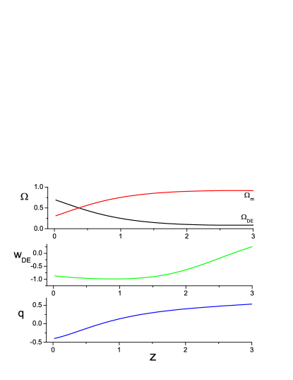
Figure 1: The late-time cosmological evolution, for Model 1, for the parameter choice $\zeta=10$ (in units where the gravitational constant is set to one), having imposed $\Omega_{m0}\approx 0.3$, $\Omega_{DE0}\approx 0.7$ at present, and having set the present scale factor $a_{0}=1$. As independent variable we use the redshift $z=-1+a_{0}/a$. In the upper graph we depict the evolution of the matter and dark energy density parameters. In the middle graph we present the evolution of the dark-energy equation-of-state parameter $w_{DE}$. In the lower graph we depict the evolution of the deceleration parameter $q$.

In summary, the cosmological behavior of the scenario at hand is in agreement with observations. We stress here that we have not considered an explicit cosmological constant, and thus the obtained acceleration arises solely from the novel, higher-derivative terms of the gravitational scalar-tensor theories.

Let us now investigate how the model parameter $\zeta$ affects the behavior of the dark-energy equation-of-state parameter $w_{DE}$. In Fig. 2 we present the evolution of $w_{DE}$ for various values of $\zeta$ (we consider $\zeta>0$ in order for the $\phi$ field not to exhibit an effective ghost behavior in (25)). As we observe, $w_{DE}$ lies in the quintessence regime and with increasing $\zeta$ its final value comes closer to the cosmological-constant value $-1$.

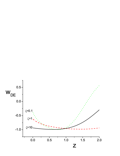
Figure 2: The evolution of the dark-energy equation-of-state parameter $w_{DE}$ as a function of the redshift $z=-1+a_{0}/a$, for six values of the model parameter $\zeta$ (in units where the gravitational constant is set to one), having imposed $\Omega_{m0}\approx 0.3$, $\Omega_{DE0}\approx 0.7$ at present, and having set the present scale factor $a_{0}=1$.

III.2 Model 2: $\mathcal{K}(\phi,B)=\frac{\phi}{2}$ and $\mathcal{G}(\phi,B)=\xi B$

As a second example we consider the case where

$$\mathcal{K}(\phi,B)=\frac{1}{2}\phi\quad\text{and}\quad\mathcal{G}(\phi,B)=\xi B,$$ (31)

with $\xi$ the corresponding coupling constant (in FRW geometry we have $B(t)=-2e^{\sqrt{\frac{2}{3}}\chi}\dot{\phi}^{2}$). Thus, the Friedmann equations (12),(13) become

$$\!\!\!\!\!\!\!\!\!\!\!\!\!\!\!\!\!3H^{2}-\rho_{m}-\frac{1}{2}\dot{\chi}^{2}+\frac{1}{8}e^{-2\sqrt{\frac{2}{3}}\chi}\left(1-2e^{\sqrt{\frac{2}{3}}\chi}\right)\phi$$

$$\ \ \ \ \ \,+\xi\dot{\phi}^{3}\left(\sqrt{6}\dot{\chi}-6H\right)=0,$$ (32)

$$\!\!\!\!\!\!\!\!\!\!\!\!\!\!\!\!\!3H^{2}+2\dot{H}+p_{m}+\frac{1}{2}\dot{\chi}^{2}+\frac{1}{8}e^{-2\sqrt{\frac{2}{3}}\chi}\left(1-2e^{\sqrt{\frac{2}{3}}\chi}\right)\phi$$

$$\ \ \ \ \ \,-\frac{1}{3}\xi\dot{\phi}^{2}\left(\sqrt{6}\dot{\phi}\dot{\chi}+6\ddot{\phi}\right)=0,$$ (33)

while the two scalar field equations (14) and (15) read as

$$\!\!\!\!\!\!\!\!\!\!\!\!\!\!\!\!\!\!\!\!\!\!\!\!\!\ddot{\chi}+3H\dot{\chi}+\frac{1}{2\sqrt{6}}e^{-2\sqrt{\frac{2}{3}}\chi}\left(1-e^{\sqrt{\frac{2}{3}}\chi}\right)\phi$$

$$-\sqrt{6}\,\xi\dot{\phi}^{2}\left(H\dot{\phi}+\ddot{\phi}\right)=0,$$ (34)

$$\!\!\!\!\!\!\!\!\!\!\xi\dot{\phi}\left\{2\left(-6H+\sqrt{6}\dot{\chi}\right)\ddot{\phi}\right.$$

$$\left.+\dot{\phi}\left[-6\dot{H}+3H\left(-6H+\sqrt{6}\dot{\chi}\right)+\sqrt{6}\ddot{\chi}\right]\right\}$$

$$\!\!\!\!\!\!\!\!\!+\frac{1}{8}e^{-2\sqrt{\frac{2}{3}}\chi}\left(1-2e^{\sqrt{\frac{2}{3}}\chi}\right)=0.$$ (35)

Therefore, in this case the effective dark-energy energy density and pressure (III),(III) write as

$$\!\!\!\!\!\!\!\!\!\!\!\!\!\!\!\!\!\!\rho_{DE}=\frac{1}{2}\dot{\chi}^{2}-\frac{1}{8}e^{-2\sqrt{\frac{2}{3}}\chi}\left(1-2e^{\sqrt{\frac{2}{3}}\chi}\right)\phi$$

$$-\xi\dot{\phi}^{3}\left(\sqrt{6}\dot{\chi}-6H\right),$$ (36)

$$\!\!\!\!\!\!\!\!\!\!\!\!\!\!\!\!\!\!p_{DE}=\frac{1}{2}\dot{\chi}^{2}+\frac{1}{8}e^{-2\sqrt{\frac{2}{3}}\chi}\left(1-2e^{\sqrt{\frac{2}{3}}\chi}\right)\phi$$

$$-\frac{1}{3}\xi\dot{\phi}^{2}\left(\sqrt{6}\dot{\phi}\dot{\chi}+6\ddot{\phi}\right).$$ (37)

In Fig. 3 we depict the cosmological evolution for the parameter choice $\xi=-1$. In the upper graph we show the behavior of the matter and dark energy density parameters, which is in agreement with the observed one Ade:2013sjv . In the middle graph of Fig. 3 we depict the evolution of the dark-energy equation-of-state parameter $w_{DE}$, which presents a dynamical behavior, and at late times it almost stabilizes in a value very close to the cosmological-constant one, as expected from observations. Finally, in the lower graph of Fig. 3 we present the evolution of the deceleration parameter, from which we can see the passage from deceleration to acceleration. Similarly to Model 1 of the previous subsection, we mention that the onset of acceleration is a pure effect of the novel, higher-derivative terms of the gravitational scalar-tensor theories.

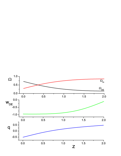
Figure 3: The late-time cosmological evolution, for Model 2, for the parameter choice $\xi=-1$ (in units where the gravitational constant is set to one), having imposed $\Omega_{m0}\approx 0.3$, $\Omega_{DE0}\approx 0.7$ at present, and having set the present scale factor $a_{0}=1$. As independent variable we use the redshift $z=-1+a_{0}/a$. In the upper graph we depict the evolution of the matter and dark energy density parameters. In the middle graph we present the evolution of the dark-energy equation-of-state parameter $w_{DE}$. In the lower graph we depict the evolution of the deceleration parameter $q$.

In order to see how the model parameter $\xi$ affects the behavior of $w_{DE}$, in Fig. 4 we present the evolution of $w_{DE}$ for various values of $\xi$. As we can see, for large negative $\xi$-values $w_{DE}$ lies in the quintessence regime, while for small negative values it exhibits the phantom-divide crossing and lies below $-1$ at current times. Although this phantom behavior might be a signal that the $\phi$ field behaves effectively as a ghost, this does not need necessarily to be the case since $\phi$-field’s effective kinetic energy in (III.2) has a complicated form depending on the time-derivatives of both fields as well as of the scale factor, and thus the phantom behavior can result even if the fields behave as canonical ones Nojiri:2013ru . Clearly, the safe procedure to investigate this issue is to perform a detailed hamiltonian analysis, a task that lies beyond the scope of the present work and thus it is left for a future project.

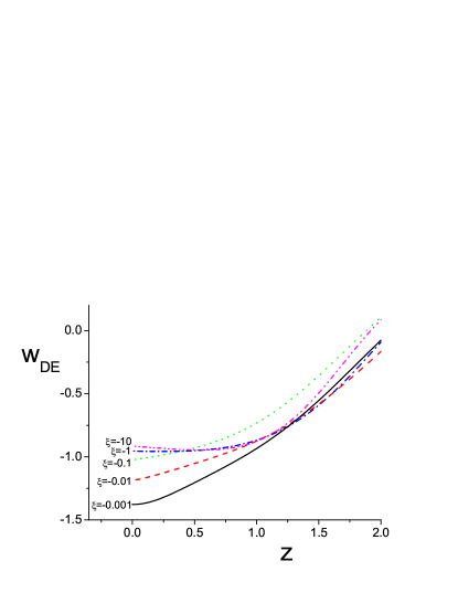
Figure 4: The evolution of the dark-energy equation-of-state parameter $w_{DE}$ as a function of the redshift $z=-1+a_{0}/a$, for five values of the model parameter $\xi$ (in units where the gravitational constant is set to one), having imposed $\Omega_{m0}\approx 0.3$,$\Omega_{DE0}\approx 0.7$ at present, and having set the present scale factor $a_{0}=1$.

IV Conclusions

New gravitational scalar-tensor theories are novel modifications of gravity possessing $2+2$ propagating degrees of freedom. Although similar models had been constructed in the scalar-field language, for instance in bi-scalar or bi-Galileon models, it is not straightforward to develop them in the pure gravitational language. However, such a construction is indeed possible using the Ricci scalar and its first and second derivatives under a specific Lagrangian that is free of ghosts Naruko:2015zze . The crucial point is that although in simple $f(R)$ theories the conformal transformation leads to the replacement of the functional degree of freedom of $f(R)$ by a scalar field, in the above constructions the derivatives of $R$ are not replaced by derivatives of the scalar-field in a naive way, but only through a specific and suitable two-field combination.

In this work we investigated the cosmological applications of new gravitational scalar-tensor theories. Introducing the matter sector and considering a homogeneous and isotropic geometry, we extracted the Friedmann equations, as well as the evolution equations of the new extra scalar degrees of freedom. In such a scenario, we obtain an effective dark energy sector that consists of both extra scalar degrees of freedom, and hence we can determine various observables, such as the dark-energy and matter density parameters, the dark-energy equation-of-state parameter and the deceleration parameter.

We analyzed two specific models, corresponding to the first non-trivial extensions of general relativity possessing $2+2$ degrees of freedom. As we showed, the resulting cosmological behavior is in agreement with observations, i.e. we obtain the transition from the matter to the dark energy era, with the onset of cosmic acceleration. Moreover, the equation-of-state parameter of the effective dark energy sector can be stabilized in a value very close to the cosmological-constant one. The most interesting feature is that such a behavior arises solely from the novel, higher-derivative terms of the gravitational scalar-tensor theories, since we have not considered an explicit cosmological constant. Additionally, we saw that for a particular range of the model parameters, the dark-energy equation-of-state parameter can exhibit the phantom-divide crossing in the recent cosmological past and currently lie in the phantom regime, which might be the case according to observations. This feature reveals the capabilities of new gravitational scalar-tensor theories, since the phantom behavior could be obtained even if the fields behave as canonical ones.

The above features indicate that the new gravitational scalar-tensor theories provide an interesting candidate for modified theories of gravity. Hence it would be worthy to perform detailed investigations on their applications. Firstly, one should perform a detail confrontation with observational data from Type Ia Supernovae (SNIa), Baryon Acoustic Oscillations (BAO), and Cosmic Microwave Background (CMB) observations, to constrain the possible classes of such modifications. Additionally, one should perform a complete phase-space analysis, in order to extract information about the global late-time behavior of the above scenarios. Moreover, an extensive analysis of the perturbations is a necessary task that could bring these constructions closer to detailed data such as those related to the growth index and the large-scale structure. Furthermore, one should examine the black hole solutions in the framework of new gravitational scalar-tensor theories, in order to obtain additional information on their novel features. Finally, one could try to analyze further extensions along this direction, using for instance terms of the form $(\nabla_{\mu}\nabla_{\nu}R)^{2}=\nabla_{\mu}\nabla_{\nu}R\nabla^{\mu}\nabla^{\nu}R$. These projects are left for near-future investigations.

References

• (1) K. A. Olive, Phys. Rept.  190, 307 (1990).
• (2) N. Bartolo, E. Komatsu, S. Matarrese and A. Riotto, Phys. Rept.  402, 103 (2004).
• (3) E. J. Copeland, M. Sami and S. Tsujikawa, Int. J. Mod. Phys.  D 15, 1753 (2006).
• (4) Y. F. Cai, E. N. Saridakis, M. R. Setare and J. Q. Xia, Phys. Rept.  493, 1 (2010).
• (5) S. Nojiri and S. D. Odintsov, eConf C0602061, 06 (2006), Int. J. Geom. Meth. Mod. Phys. 4, 115 (2007).
• (6) S. Capozziello and M. De Laurentis, Phys. Rept.  509, 167 (2011).
• (7) K. S. Stelle, Phys. Rev. D 16, 953 (1977).
• (8) T. Biswas, E. Gerwick, T. Koivisto and A. Mazumdar, Phys. Rev. Lett.  108, 031101 (2012).
• (9) T. P. Sotiriou and V. Faraoni, Rev. Mod. Phys.  82, 451 (2010).
• (10) A. De Felice and S. Tsujikawa, Living Rev. Rel.  13, 3 (2010).
• (11) S. ’i. Nojiri and S. D. Odintsov, Phys. Rept.  505, 59 (2011).
• (12) S. Nojiri and S. D. Odintsov, Phys. Rev. D 74, 086005 (2006).
• (13) S. ’i. Nojiri and S. D. Odintsov, Phys. Lett. B 631, 1 (2005).
• (14) A. De Felice and S. Tsujikawa, Phys. Lett. B 675, 1 (2009).
• (15) D. Lovelock, J. Math. Phys.  12, 498 (1971).
• (16) N. Deruelle and L. Farina-Busto, Phys. Rev. D 41, 3696 (1990).
• (17) P. D. Mannheim and D. Kazanas, Astrophys. J.  342, 635 (1989).
• (18) E. E. Flanagan, Phys. Rev. D 74, 023002 (2006).
• (19) G. W. Horndeski, Int. J. Theor. Phys.  10 (1974) 363.
• (20) A. Nicolis, R. Rattazzi and E. Trincherini, Phys. Rev. D 79 (2009) 064036.
• (21) C. Deffayet, G. Esposito-Farese and A. Vikman, Phys. Rev. D 79, 084003 (2009).
• (22) C. Deffayet, S. Deser and G. Esposito-Farese, Phys. Rev. D 80, 064015 (2009).
• (23) C. Deffayet, X. Gao, D. A. Steer and G. Zahariade, Phys. Rev. D 84 (2011) 064039.
• (24) M. Zumalacárregui and J. García-Bellido, Phys. Rev. D 89, 064046 (2014).
• (25) J. Gleyzes, D. Langlois, F. Piazza and F. Vernizzi, Phys. Rev. Lett.  114, no. 21, 211101 (2015).
• (26) X. Gao, Phys. Rev. D 90, 081501 (2014).
• (27) J. Gleyzes, D. Langlois, F. Piazza and F. Vernizzi, JCAP 1502, 018 (2015).
• (28) X. Gao, Phys. Rev. D 90, 104033 (2014).
• (29) A. Padilla, P. M. Saffin and S. Y. Zhou, JHEP 1012 (2010) 031.
• (30) A. Padilla and V. Sivanesan, JHEP 1304 (2013) 032.
• (31) V. Sivanesan, Phys. Rev. D 90 (2014) 10, 104006.
• (32) T. Kobayashi, N. Tanahashi and M. Yamaguchi, Phys. Rev. D 88 (2013) 8, 083504.
• (33) S. Ohashi, N. Tanahashi, T. Kobayashi and M. Yamaguchi, JHEP 1507 (2015) 008.
• (34) A. Padilla, D. Stefanyszyn and M. Tsoukalas, Phys. Rev. D 89 (2014) 6, 065009.
• (35) A. Padilla, P. M. Saffin and S. Y. Zhou, JHEP 1101, 099 (2011).
• (36) C. Charmousis, T. Kolyvaris, E. Papantonopoulos and M. Tsoukalas, JHEP 1407 (2014) 085.
• (37) A. Naruko, D. Yoshida and S. Mukohyama, arXiv:1512.06977 [gr-qc].
• (38) P. A. R. Ade et al. [Planck Collaboration], Astron. Astrophys.  571, A1 (2014).
• (39) S. Nojiri and E. N. Saridakis, Astrophys. Space Sci.  347, 221 (2013).