On rank one perturbations of Hamiltonian system with periodic coefficients

1 Introduction

Let $J,W\in\mathbb{R}^{2N\times 2N}$ be two matrices such that $J$ is nonsingular and skew-symmetric matrix. We say that the matrix $W$ is $J$-symplectic (or $J$-orthogonal ) if $W^{T}JW=J$. These types of matrices (so-called structured) usually appear in control theory [15, 12, 11, 1]: more precisely in optimal control [11] and in the parametric resonance theory [10, 15]. In these areas, these types of matrices are obtained as solutions of Hamiltonian systems with periodic coefficients. About these systems, that are differential equations with $P$-periodic coefficients of the below form

$$J\dfrac{dX(t)}{dt}=H(t)X(t),\;\;t\in\mathbb{R}$$ (1)

where $J^{T}=-J$, $(H(t))^{T}=H(t)=H(t+P)$. The fundamental solution $X(t)$ of (1) i.e. the matrix satisfying

$$\left\{\begin{array}[]{rcl}J\dfrac{dX(t)}{dt}&=&H(t)X(t),\;\;t\in\mathbb{R}_{+}^{*}\\ X(0)&=&I_{2N}\end{array}\right.$$ (2)

is $J$-symplectic [2, 7, 3, 15] and satisfies the relationship $X(t+nP)=X(t)X^{n}(P)$, $\forall t\in\mathbb{R}$ and $\forall n\in\mathbb{N}$. The solution of the system evaluated at the period is called the monodromy matrix of the system. The eigenvalues of this monodromy matrix are called the multipliers of the system (2). The following definition permits to classify the multiplies of Hamiltonian system

Definition 1

Let $\rho$ be a semi-simple multiplier of (2) lying on the unit circle. Then $\rho$ is called a multiplier of the first (second ) kind if the quadratic form $(iJx,x)$ is positive (negative) on the eigenspace associated with $\rho$ . When $(Jx,x)=0$, then $\rho$ is of mixed kind.

In this definition, the notation $(iJx,x)$ stands for the Euclidean scalar product and $i=\sqrt{-1}$.

This other definition proposed by S. K. Godunov [4, 5, 8, 9] gives another classification of the multipliers of (2)

Definition 2

Let $\rho$ be a semi-simple multiplier of (2) lying on the unit circle. We say that $\rho$ is of the red (green) color or in short $r$-multiplier ( $g$-multiplier) if $(S_{0}x,x)>0$ ( respectively $(S_{0}x,x)<0$ ) on the eigenspace associated with $\rho$ where $S_{0}=(1/2)\left((JX(P))^{T}+(JX(P))\right)$. If $(S_{0}x,x)=0$, we say that $\rho$ is of mixed color.

From Definition 2, Dosso and Sadkane obtained a result of strong stability of symplectic matrix (see [2, 6, 4])

Theorem 3

A symplectic matrix is strong stability if and only if

1. all eigenvalues are on the unit circle ;

2. the eigenvalues are either red color or green color ;

3. the subspaces associated of these deux groups of the eigenvalues are well separated.

Denote by $\mathbb{P}_{r}$ and $\mathbb{P}_{g}$ the spectral projectors associated with the $r-$eigenvalues and $r-$eigenvalues of the monodromy matrix $X(P)$ of (2) and let’s put $S_{r}:=\mathbb{P}_{r}^{T}S_{0}\mathbb{P}_{r}=S_{r}^{T}\geq 0$ and $S_{g}:=\mathbb{P}_{g}^{T}S_{0}\mathbb{P}_{g}=S_{g}^{T}\leq 0$ where $S_{0}=(1/2)\left((X(P)J)+(X(P)J)^{T}\right)$. We give the following theorem which gathers all assertions on the strong stability of Hamiltonian systems with periodic coefficients [15, 6, 2].

Theorem 4

The Hamiltonian system (2) is strongly stable if one of the following conditions is satisfied :

1. If there exists $\epsilon>0$ such that any Hamiltonian system with $P$-periodic coefficients of the form $J\dfrac{dx(t)}{dt}=\widetilde{H}(t)x(t)$ and satisfying

   $$\|H-\widetilde{H}\|\equiv\int_{0}^{T}\|H(t)-\widetilde{H}(t)\|dt<\epsilon$$

   is stable.

2. The monodromy matrix $W=X(P)$ of the system (2) is strongly stable

3. (KGL criterion) the multipliers of the system (2) are either of the first kind and either of second kind. The multipliers of the first kind and second kind of the monodromy matrix should be well separated i.e. the quantity

   $$\delta_{KGL}(X(P))=min\left\{|e^{i\theta_{k}}-e^{i\theta_{l}}|\;;e^{i\theta_{k}},e^{i\theta_{l}}\right.$$

   $$\left.\text{are multipliers of $(\ref{EQS1})$ of different kinds }\right\}$$ (3)

   should not be close to zero.

4. the multipliers of the system (2) are either of the red color and either of the green color. The r-multipliers and g-multipliers of the monodromy matrix should be well separated i.e. the quantity

   $$\delta_{S}(X(P))=min\left\{|e^{i\theta_{k}}-e^{i\theta_{l}}|\;;e^{i\theta_{k}},e^{i\theta_{l}}\right.$$

   $$\left.\text{are $r-$multpliers and $g-$multipliers of}\;\;(\ref{EQS1})\right\}$$ (4)

   should not be close to zero.

5. $S_{r}\geq 0$, $S_{g}\leq 0$ and $S_{r}-S_{g}>0$

6. $\mathbb{P}_{r}+\mathbb{P}_{g}=I$ and $\mathbb{P}_{r}^{T}S_{0}\mathbb{P}_{g}=0$.

The paper is organized as follows. In Section 2 we give some preliminaries and useful results to introduce the rank one perturbations of Hamiltonian systems with periodic coefficients. More specifically, this section explains what led us to rank one perturbations of Hamiltonian system with periodic coefficients. Section 3 explains the concept of rank one perturbation of Hamiltonian systems with coefficients. In Section 4 we analyze the consequences of strongly stable of Hamiltonian systems with periodic coefficients on its rank on perturbation. Section 5 is devoted to numerical tests. Finally some concluding remarks are summarized in Section 6

Throughout this paper, we denoted the identity and zero matrices of order $k$ by $I_{k}$ and $0_{k}$ respectively or just $I$ and $0$ whenever it is clear from the context. The 2-norm of a matrix $A$ is denoted by $\|A\|$. The transpose of a matrix (or vector ) $U$ is denoted by $U^{T}$.

2 Rank one perturbation of symplectic matrices depending on a parameter

Let $W\in\mathbb{R}^{2N\times 2N}$ be a $J$-symplectic matrix where $J\in\mathbb{R}^{2N\times 2N}$ is skew-symmetric matrix (i.e. $J^{T}=-J$)[13, 14].

Definition 5

We call a rank one perturbation of the symplectic matrix $W$ any matrix of the form $\widetilde{W}=(I+uu^{T}J)W$ where $u\in\mathbb{R}^{2N}$.

We recall in the following proposition some properties of rank one perturbations of symplectic matrices (see [16]).

Proposition 6

Let $W$ be a $J$-sympectic matrix.

1. Any rank one perturbation of $W$ is $J$-symplectic.

2. The invertible of a rank one perturbation $I+uu^{T}J$ of identity matrix $I$ is the matrix $I-uu^{T}J$.

Proof:  See [13, 16] for the proof. $\sqcap\!\!\!\!\sqcup$

Let $u$ be a vector of $\mathbb{R}^{2N}$. Consider the following lemma

Lemma 7

Consider the rank one perturbations $\widetilde{W}=(I+uu^{T}J)W$ of the $J$-symplectic matrix $W$. Then for any $y\in\mathbb{R}^{2N}$, the quadratic form $(S_{0}y,y)$ is defined by

$$(S_{0}y,y)=(\widetilde{S}_{0}y,y)-\varphi(y)$$ (5)

where

$$\widetilde{S}_{0}=(1/2)\left((J\widetilde{W})+(J\widetilde{W})^{T}\right)$$

and

$$\varphi(y)=(1/2)\left(((Juu^{T}JW)+(Juu^{T}JW))^{T})y,y\right).$$

Proof:  Developing $\widetilde{S}_{0}$, we have

$$\widetilde{S}_{0}= (1/2)\left((JW)+(JW)^{T}\right)+$$

$$(1/2)\left[(Juu^{T}JW)+(Juu^{T}JW)^{T}\right].$$

we deduct

$$(\widetilde{S}_{0}y,y)=(S_{0}y,y)+$$

$$\underbrace{(1/2)\left(\left[(Juu^{T}JW)+(Juu^{T}JW)^{T}\right]y,y\right)}_{\displaystyle\varphi(y)}$$

$$\qquad=(S_{0}y,y)+\varphi(y)$$

$\sqcap\!\!\!\!\sqcup$

Corollary 8

Let $\rho$ be an eigenvalue of $W$ of modulus 1 and $y$ an eigenvector associated with $\rho$. Then $\rho$ is an eigenvalue of red color (respectively eigenvalue of green ) if and only if $\left(\widetilde{S}_{0}y,y\right)>\varphi(y)$ (respectively $\left(\widetilde{S}_{0}y,y\right)<\varphi(y)$).
However if $\left(\widetilde{S}_{0}y,y\right)=\varphi(y)$, then $\rho$ is of mixed color.

Proof:  According to lemma 7, we get

$$(S_{0}y,y)=(\widetilde{S}_{0}y,y)-\varphi(y)$$

From Definition 2, we have

• if $\rho$ is an eigenvalue of red color,

  $$(S_{0}y,y)>0\Longrightarrow(\widetilde{S}_{0}y,y)>\varphi(y)\;;$$

• if $\rho$ is an eigenvalue of green color,

  $$(S_{0}y,y)<0\Longrightarrow(\widetilde{S}_{0}y,y)<\varphi(y)\;;$$

• if $\rho$ is an eigenvalue of mixed color,

  $$(S_{0}y,y)=0\Longrightarrow(\widetilde{S}_{0}y,y)=\varphi(y).$$

$\sqcap\!\!\!\!\sqcup$

We consider the following rank one perturbation of the fundamental solution $X(t)$ of (2)

$$\widetilde{X}(t)=(I+uu^{T})X(t)$$ (6)

then we have the following lemma

Lemma 9

If $\widetilde{X}(t)$ is a $J$-symplectic matrix function such that $\text{rank}(\widetilde{X}(t)-X(t))=1,\;\,\forall t>0$, then there is a vector function $u(t)\in\mathbb{C}^{2N}\;\;\;\forall t>0$ such that

$$\widetilde{X}(t)=(I+u(t)u(t)^{T}J)X(t),\;\;\forall t\in\mathbb{R}$$

Conversely, for any vector $u(t)\in\mathbb{C}^{2N}$, the matrix function $\widetilde{X}(t)$ is $J$-symplectic.

Proof:  According to Lemma 7.1 of [13, Section 7,p. 18], for all $t>0$, there exists a vector $u(t)\in\mathbb{C}^{2N}$ such that

$$\widetilde{X}(t)=(I+u(t)u(t)^{T}J)X(t).$$

Moreover, if $X(t)$ is $J$-symplectic, $\widetilde{X}(t)$ is also $J$-symplectic. $\sqcap\!\!\!\!\sqcup$

This Lemma leads us to introduce the concept of rank one perturbation of Hamiltonian systems with periodic coefficients.

Now consider, in the follow, that the vector function is a vector constant. We give the following theorem which extend Theorem 7.2 of [13, Section 7, p. 19] to matrizant of system (2).

Theorem 10

Let $J\in\mathbb{C}^{2N\times 2N}$ be skew-symmetric and nonsingular matrix, $(X(t))_{t>0}$ fondamental solution of system (2) and $\lambda(t)\in\mathbb{C}$ an eigenvalue of $X(t)$ for all $t>0$. Assume that $X(t)$ has the Jordan canonical form

$$\left(\bigoplus_{j=1}^{l_{1}}\mathcal{J}_{n_{1}}(\lambda(t))\right)\oplus\left(\bigoplus_{j=1}^{l_{2}}\mathcal{J}_{n_{2}}(\lambda(t))\right)\oplus\cdots\oplus\left(\bigoplus_{j=1}^{l_{m(t)}}\mathcal{J}_{n_{m(t)}}(\lambda(t))\right)\oplus\mathcal{J}(t),$$

where $n_{1}>\cdots>n_{m(t)}$ with $m\;:\;\mathbb{R}\longrightarrow\mathbb{N}^{*}$ a function of index such that the algebraic multiplicities is $a(t)=l_{1}n_{1}+\cdots+l_{m(t)}n_{m(t)}$ and $\mathcal{J}(t)$ with $\sigma(\mathcal{J}(t))\subseteq\mathbb{C}\setminus\{\lambda(t)\}$ contains all Jordan blocks associated with eigenvalues different from $\lambda(t)$. Furthermore, let $u\in\mathbb{C}^{2N}$ and $B(t)=uu^{T}JX(t)$.

1. If $\forall t>0$, $\lambda(t)\not\in\{-1,1\}$, then generically with respect to the components of $u$, the matrix $X(t)+B(t)$ has the Jordan canonical form

   $$\left(\bigoplus_{j=1}^{l_{1}-1}\mathcal{J}_{n_{1}}(\lambda(t))\right) \oplus\left(\bigoplus_{j=1}^{l_{2}}\mathcal{J}_{n_{2}}(\lambda(t))\right)\oplus\cdots\oplus$$

   $$\left(\bigoplus_{j=1}^{l_{m(t)}}\mathcal{J}_{n_{m(t)}}(\lambda(t))\right)\oplus\widetilde{\mathcal{J}}(t),$$ (7)

   where $\mathcal{J}(t)$ contains all the Jordan blocks of $X(t)+B(t)$ associated with eigenvalues different from $\lambda(t)$.

2. If $\exists t_{0}>0$, verifying $\lambda(t_{0})\in\{+1,1\}$, we have

   1. if $n_{1}$ is even, then generically with respect to the components of $u$, the matrix
      $X(t_{0})+B(t_{0})$ has the Jordan canonical form

      $$\left(\bigoplus_{j=1}^{l_{1}-1}\mathcal{J}_{n_{1}}(\lambda(t_{0}))\right) \oplus\left(\bigoplus_{j=1}^{l_{2}}\mathcal{J}_{n_{2}}(\lambda(t_{0}))\right)\oplus\cdots\oplus$$

      $$\left(\bigoplus_{j=1}^{l_{m(t)}}\mathcal{J}_{n_{m(t)}}(\lambda(t_{0}))\right)\oplus\widetilde{\mathcal{J}}(t_{0}),$$

      where $\mathcal{J}(t)$ contains all the Jordan of $X(t)+B(t)$ associated with eigenvalues different from $\lambda(t)$.

   2. if $n_{1}$ is odd, then $l_{1}$ is even and generically with respect to the components of $u$, the matrix $X(t_{0})+B(t_{0})$ has the Jordan canonical form

      $$\mathcal{J}_{n_{1}+1}(\lambda(t_{0})) \oplus\left(\bigoplus_{j=1}^{l_{1}-2}\mathcal{J}_{n_{1}}(\lambda(t_{0}))\right)\oplus\cdots\oplus$$

      $$\left(\bigoplus_{j=1}^{l_{m(t)}}\mathcal{J}_{n_{m(t)}}(\lambda(t_{0}))\right)\oplus\widetilde{\mathcal{J}}(t_{0}),$$

      where $\mathcal{J}(t_{0})$ contains all the blocks of $X(t_{0})+B(t_{0})$ associated with eigenvalues different from $\lambda(t_{0})$.

Proof:  For all $t>0$, if $\lambda(t)\not\in\{-1,1\}$, we have the decomposition $(\ref{EQS2})$ according to [13, Theorem 7.2]). Other hand, the number of Jordan blocks depend on the variation of $t$. Thus, this number is a function of index $m\;:\;\mathbb{R}^{+}\longrightarrow\mathbb{N}^{*}$.
For the other two points $(2a)$ and $(2b)$, they show in the same way that items (2) and (3) of Theorem 7.2 of [13, Theorem 7.2]) since $X(t_{0})+B(t_{0})$ is a constant matrix. $\sqcap\!\!\!\!\sqcup$

In reality, the integers $l_{1},...,l_{m}(t)$ and indexes $n_{1},...,n_{m}(t)$ are not constant when t varies. The number of Jordan blocks and their sizes can varied in function of the variation of t. In Theorem 10, we considered the integers $l_{k}$ and $n_{k}$ constant $\forall k\in\left\{1,...,m(t)\right\}$ for an index $m(t)$ given. When $t=0$, $\lambda(0)=1$ with $m(0)=2N$ and $l_{k}=1,\;\;\forall k$. All Jordan blocks are reduced to $1$.

3 Rank one perturbations of Hamiltonian system with periodic coefficients

Let $u$ be a constant vector of $\mathbb{R}^{2N}$. $(X(t))_{t\in\geq 0}$ the fundamental solution of system 2. We have the following proposition

Proposition 11

Consider the perturbed Hamiltonian system

$$J\dfrac{d\widetilde{X}(t)}{dt}=\left[H(t)+E(t)\right]\widetilde{X}(t)$$ (8)

where

$$E(t)=(Juu^{T}H(t))^{T}+Juu^{T}H(t)+(uu^{T}J)^{T}H(t)(uu^{T}J).$$

Then $\widetilde{X}(t)=(I+uu^{T}J)X(t)$ is a solution of system (8).

Proof:  By derivation of $\widetilde{X}(t)$, we obtain :

$$J\dfrac{d\widetilde{X}(t)}{dt}= J(I+uu^{T}J)J^{-1}J\dfrac{dX(t)}{dt}$$

$$= J(I+uu^{T}J)J^{-1}H(t)X(t),$$

$$\text{according from system }\;\;(\ref{EQS1})$$

$$= [H(t)+Juu^{T}H(t)]X(t)$$

$$= [H(t)+Juu^{T}H(t)](I+uu^{T}J)^{-1}\widetilde{X}(t)$$

$$= [H(t)+Juu^{T}H(t)](I-uu^{T}J)\widetilde{X}(t)$$

because $$(I+uu^{T}J)^{-1}=(I-uu^{T}J)\;\;\;(\text{see \cite[cite]{[\@@bibref{}{Yan2}{}{}]}})$$

$$= \left[H(t)-H(t)uu^{T}J+Juu^{T}H(t)-\right.$$

$$\left.Juu^{T}H(t)uu^{T}J\right]\widetilde{X}(t)$$

$$= \left[H(t)+\underbrace{(Juu^{T}H(t))^{T}+Juu^{T}H(t)+(uu^{T}J)^{T}H(t)(uu^{T}J)}_{\displaystyle E(t)}\right]\widetilde{X}(t)$$

Hence the following perturbed Hamiltonian equation (8) where

$$E(t)= (Juu^{T}H(t))^{T}+Juu^{T}H(t)+$$

$$(uu^{T}J)^{T}H(t)(uu^{T}J)$$ (9)

$\sqcap\!\!\!\!\sqcup$

We note that $E(t)$ is symmetric and $P$-periodic i.e. $E(t)^{T}=E(t)$ and $E(t+P)=E(t)$ for all $t\in\geq 0$. The following corollary gives us a simplified form of system (8)

Corollary 12

The system (8) can be put at the form

$$\left\{\begin{array}[]{rcl}J\dfrac{d\widetilde{X}(t)}{dt}&=&(I-uu^{T}J)^{T}H(t)(I-uu^{T}J)\widetilde{X}(t),\\ &&\\ \widetilde{X}(0)&=&I+uu^{T}J\end{array}\right.$$ (10)

Proof:  Indeed, developing
$(I-uu^{T}J)^{T}H(t)(I-uu^{T}J)$ and we get

$$(I-uu^{T}J)^{T}H(t)(I-uu^{T}J)=H(t)+$$

$$\underbrace{(J^{T}uu^{T}H(t))^{T}+J^{T}uu^{T}H(t)+(uu^{T}J)^{T}H(t)(uu^{T}J)}_{E(t)}$$

and $\widetilde{X}(0)=(I+uu^{T}J)X(0)=I+uu^{T}J$. $\sqcap\!\!\!\!\sqcup$

We give the following corollary

Corollary 13

Let $(X(t))_{t\geq 0}$ be the fundamental solution of system (2).
All solution $\widetilde{X}(t)$ of perturbed system (10) of system (2), is of the form $\widetilde{X}(t)=(I+uu^{T}J)X(t)$.

Proof:  From Proposition 8 if $X(t)$ is a solution de (2), the perturbed matrix $W(t)=(I+uu^{T}J)X(t)$ is a solution of (10).
Reciprocally, for any solution $\widetilde{X}(t)$ de $(\ref{Eq2})$, Let’s put

$$X(t)=(I-uu^{T}J)\widetilde{X}(t)$$

where $u$ is the vector defined in system (10)

$$\Longrightarrow\widetilde{X}(t)=(I+uu^{T}J)X(t)$$

because $(I+uu^{T}J)$ is inverse of the matrix
$(I-uu^{T}J)$ (see [16]). By replacing this expression $\widetilde{X}(t)$ in (10), we obtain

$$J(I+uu^{T}J)\dfrac{d}{dt}X(t)=(I-uu^{T}J)^{T} H(t)X(t)$$

$$J(I+uu^{T}J)\dfrac{d}{dt}X(t)=(I-uu^{T}J)^{T} H(t)X(t)$$

$$(I-uu^{T}J)^{-T}J(I+uu^{T}J)\dfrac{d}{dt}X(t)= H(t)X(t)$$

$$\underbrace{(I+uu^{T}J)^{T}J(I+uu^{T}J)}_{=J}\dfrac{d}{dt}X(t)= H(t)X(t)$$

$$J\dfrac{d}{dt}X(t)= H(t)X(t)$$

and $X(0)=(I-uu^{T}J)\widetilde{X}(0)=(I-uu^{T}J)(I+uu^{T}J)=I$. Consequently, $X(t)$ is solution of (2). $\sqcap\!\!\!\!\sqcup$

From the foregoing, we give the following definition :

Definition 14

We call rank one perturbations of Hamiltonian system with periodic coefficients, any perturbation of the form (10) of (2).

Consider the following canonical perturbed system taking $I_{2N}$ at $t=0$.

$$\left\{\begin{array}[]{rcl}J\dfrac{d\widetilde{W}(t)}{dt}&=&(I-uu^{T}J)^{T}H(t)(I-uu^{T}J)\widetilde{W}(t),\\ &&\\ \widetilde{W}(0)&=&I\end{array}\right.$$ (11)

4 Consequence of the strong stability on rank one perturbations

We give the following proposition which is a consequent of Corollary 8

Proposition 15

If a symplectic matrix $W$ is strongly stable, then there exists a positif constant $\delta$ such that any vector $u\in\mathbb{R}^{2N}$ verifying $\|uu^{T}JW\|<\delta$, we have $\left(\widetilde{S}_{0}y,y\right)\not=\varphi(y)$ for any eigenvector $y$ of $W$ where $\widetilde{S}_{0}=(1/2)\left((J\widetilde{W})+(J\widetilde{W})\right)$ with $\widetilde{W}=(I+uu^{T})W$.

Proof:  The strong stability of symplectic matrix $W$ implies that the eigenvalues of $W$ are either of red color either of green color i.e. for any eigenvector $y$ of $W$, we have

$$(S_{0}y,y)\neq 0\Longrightarrow(\widetilde{S}_{0}y,y)\neq\varphi(y)$$

using Corollary 8. $\sqcap\!\!\!\!\sqcup$

This following Proposition gives us another consequence of the strong stability of $W$ under small perturbation that preserve symplecticity.

Proposition 16

If a symplectic matrix $W$ is strongly stable, then there exists a positif constant $\delta$ such that any vector $u\in\mathbb{R}^{2N}$ verifies $\|uu^{T}JW\|<\delta$, we have $\widetilde{W}=(I+uu^{t}J)W$ is stable.

Proof:  If $W$ is strongly stable, then there exists a positif constant $\delta$ such that any small perturbation $\widetilde{W}$ of $W$ preserving its symplecticity verifying $\|\widetilde{W}-W\|\leq\delta$, is stable. In particulary, if the perturbation is a rank one perturbation with $\widetilde{W}$ of the form $W+uu^{T}JW$, any vector $u$ verifying $\|uu^{T}JW\|\leq\delta$ gives $\widetilde{W}$ stable. $\sqcap\!\!\!\!\sqcup$

Hence we have this following result on the strong stability of the Hamiltonian systems with periodic coefficients

Proposition 17

If Hamiltonian system with periodic coefficients (2) is strongly stable, then there exists $\varepsilon>0$ such that for any vector $u$ verifying

$$\|E(t)\|\leq\varepsilon$$

where $E(t)$ is defined in (9), rank one perturbation Hamiltonian system (10) associated is stable.

Proof:  This proposition is a consequence of Theorem 4 using system (8) of Proposition 11. $\sqcap\!\!\!\!\sqcup$

On the other hand, if the unperturbed system is unstable, there exits a neighborhood in which any rank one perturbation of system (2) remains unstable.

Remark 18

The stability of any small rank one perturbation of a Hamiltonian system with periodic coefficients doesn’t imply its strong stability because we are in a particular case of the perturbation of the system. However it can permit to study the behavior of multipliers of Hamiltonian systems with periodic coefficients.

5 Numerical examples

Example 19

Consider the Mathieu equation

$$J\dfrac{d^{2}y(t)}{dt^{2}}=(a+b\sin(2t))y(t)$$ (12)

where $a,b\in\mathbb{R}$ (see [15, vol. 2, p. 412],[4]). Putting

$$x(t)=\left(\begin{array}[]{c}y\\ \dfrac{dy}{dt}\end{array}\right),J=\left(\begin{array}[]{cc}0&-1\\ 1&0\end{array}\right)$$

and

$$H(t)=\left(\begin{array}[]{cc}b\;\sin\;2t+a&0\\ 0&1\end{array}\right),$$

we obtain the following canonical Hamiltonian Equation

$$J\dfrac{dX(t)}{dt}=H(t)X(t),\quad\forall t\in\mathbb{R},X(0)=I_{2},$$ (13)

where the matrix $H(t)$ is Hamiltonian and $\pi$-periodic. Let $u\in\mathbb{R}^{2N\times 2N}$ be a random vector in a neighborhood of the zero vector. Consider perturbed system (10) of (13). We show that the rank one perturbation of the fundamental solution is a solution of perturbed system (10). Consider

$$\psi(t)=\|\widetilde{X}_{1}(t)-\widetilde{X}_{2}(t)\|,\quad\forall t\geq 0$$

where $\widetilde{X}_{1}(t)=(I-uu^{T}J)X(t)$ and $(\widetilde{X}_{2}(t))_{t\in\geq 0}$ is the solution of system (10). We show by numerical examples that $(\psi(t))\leq 1.5\;10^{-14},\;\;\forall t\in[0,\pi]$.

• For $a=7$ and $b=4$, consider the vector $u=\left(\begin{array}[]{c}0.8913\\ 0.7621\end{array}\right)$. In Figure 1, we consider a random vector u which permits to disrupt system (13) by the vectors $u,10^{-1}u,10^{-2}u$ and $10^{-3}u$. In this first figure, we note that $\psi(t)\leq 1.5\;10^{-14}$. This shows that $\widetilde{X}_{1}(t)=\widetilde{X}_{2}(t)$ for all $t\in[0,\pi]$ i.e. the rank one perturbation $(\widetilde{X}_{1}(t))_{t\in[0,\pi]}$ of the fundamental solution of system (13) is equal to the solution $(\widetilde{X}_{2}(t))_{t\in[0,\pi]}$ of rank one perturbation system (10).

  

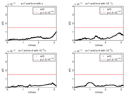
  Figure 1: Comparison of two solutions

  However, unperturbed system (13) is strongly stable. We remark that the rank one perturbed systems (10) of (13) is strongly stable when the vector $u\in\left\{u,10^{-1}u,10^{-2},10^{-3}\right\}$. Therefore they are stable. This justifies Proposition (17)

• For $a=16.1916618724166685...$ and $b=5$, consider the vector $u=\left(\begin{array}[]{c}0.4565\\ 0.0185\end{array}\right)$. In this another example illustrated by Figure 2, we consider a random vector u which permits to disrupt system (13) by the vectors $u,10^{-1}u,10^{-2}u$ and $10^{-3}u$. In figure 2, we note that $\psi(t)\leq 1.5\;10^{-14}$. This shows that $\widetilde{X}_{1}(t)=\widetilde{X}_{2}(t)$ for all $t\in[0,\pi]$.

  

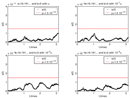
  Figure 2: Comparison of two solutions

In this example, the unperturbed system being unstable, the rank one perturbation system is unstable when the vector $u\in\left\{u,10^{-1}u,10^{-2}u,10^{-3}\right\}$. This justifies the existence of a neighborhood of the unperturbed system in which any rank one perturbation of the system is unstable.

Example 20

Consider the system of differential equations ( see [9] and [15, Vil. 2, p. 412])

$${\tiny\left\{\begin{array}[]{l}q_{1}\dfrac{d^{2}\eta_{1}}{dt^{2}}+p_{1}\eta_{1}+\left[a\eta_{1}\cos\;2\gamma t+(b\cos\;2\gamma t+c\sin\;2\gamma t)\eta_{3}\right]=0\\ q_{2}\dfrac{d^{2}\eta_{2}}{dt^{2}}+p_{2}\eta_{2}+g\eta_{3}\sin\;5\gamma t=0,\\ q_{3}\dfrac{d^{2}\eta_{3}}{dt^{2}}+p_{3}\eta_{3}+\left[(b\cos\;2\gamma t+c\sin\;2\gamma t)\eta_{1}+g\eta_{2}\sin\;5\gamma t\right]=0,\end{array}\right.}$$ (14)

which can be reduced on the following canonical Hamiltonian system

$$J\dfrac{dX(t)}{dt}=H(t),\qquad X(0)=I_{6}$$ (15)

where

$$x=\left(\begin{array}[]{c}\eta\\ \dfrac{d\eta}{dt}\end{array}\right),\qquad J=\left(\begin{array}[]{cc}0_{3}&-I_{3}\\ I_{3}&0_{3}\end{array}\right),$$

$$H(t)=\left(\begin{array}[]{cc}P(t)&0_{3}\\ 0_{3}&I_{3}\end{array}\right),$$

with $\eta=\left(\begin{array}[]{c}\frac{\eta_{1}}{\sqrt{q_{1}}}\\ \dfrac{\eta_{2}}{\sqrt{q_{2}}}\\ \dfrac{eta_{3}}{\sqrt{q_{3}}}\end{array}\right)$ and

$$P(t)=\left(\begin{array}[]{ccc}\dfrac{p_{1}+a\cos\;2\gamma t}{q_{1}}&0&\dfrac{b\cos\;2\gamma\;2\gamma t+c\sin\;2\gamma t}{\sqrt{q_{1}q_{3}}}\\ 0&\dfrac{p_{2}}{q_{2}}&\frac{g\sin\>5\gamma t}{\sqrt{q_{2}q_{3}}}\\ \dfrac{b\cos\;2\gamma\;2\gamma t+c\sin\;2\gamma t}{\sqrt{q_{1}q_{3}}}&\frac{g\sin\>5\gamma t}{\sqrt{q_{2}q_{3}}}&\dfrac{p_{3}}{q_{3}}\end{array}\right).$$

Let $u\in\mathbb{R}^{2N}$ be a random vector in a neighborhood of the zero vector. Consider perturbed system (10) of (15). We show that the rank one perturbation of the fundamental solution of 15 is a solution of its rank one perturbation system. Consider

$$\psi(t)=\|\widetilde{X}_{1}(t)-\widetilde{X}_{2}(t)\|,\forall t\in\mathbb{R}$$

where $\widetilde{X}_{1}(t)=(I-uu^{T}J)X(t)$ and $(\widetilde{X}_{2}(t))_{t\in\mathbb{R}}$ is the solution of the rank one perturbation Hamiltonian system (10) of (15). Figures 3 and 4 represent the norm of the difference between $\widetilde{X}_{1}$ et $\widetilde{X}_{2}$.

• for $\epsilon=15.5$ and $\delta=1$, Let’s take
  $u=\tiny\left(\begin{array}[]{c}0.8214\\ 0.4447\\ 0.6154\\ 0.7919\\ 0.9218\\ 0.7382\end{array}\right)$. Figure 3 is obtained for values of the vector u taken in $\left\{u,10^{-1}u,10^{-2}u,10^{-3}u\right\}$. In figure 3, we note that $\psi(t)\leq 5\;10^{-13}$. This shows that $\widetilde{X}_{1}(t)=\widetilde{X}_{2}(t)$ for all $t\in[0,\pi]$ i.e. the rank one perturbation $(\widetilde{X}_{1}(t))_{t\in[0,\pi]}$ of the fundamental solution of system (15) is equal to the solution $(\widetilde{X}_{2}(t))_{t\in[0,\pi]}$ of the rank one perturbation system of (15).

  

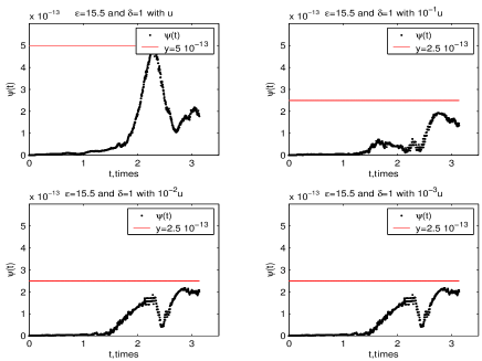
  Figure 3: Comparison of two solutions

  However, unperturbed system (15) is strongly stable. We also note that the rank one perturbed systems (10) of (15) is strongly stable when the vector $u\in\left\{u,10^{-1}u,10^{-2}u,10^{-3}\right\}$. Therefore they are stable. This justifies Proposition (17)

• $\epsilon=15$ and $\delta=2$, Let’s take $u=\tiny\left(\begin{array}[]{c}0.0272\\ 0.3127\\ 0.0129\\ 0.3840\\ 0.6831\\ 0.0928\end{array}\right)$. The following figures is obtained for values of the vector u taken in $\left\{u,10^{-1}u,10^{-2}u,10^{-3}u\right\}$. In figure 4, we also note that $\psi(t)\leq 2\;10^{-13}$. This shows that $\widetilde{X}_{1}(t)=\widetilde{X}_{2}(t)$ for all $t\in[0,\pi]$.

  

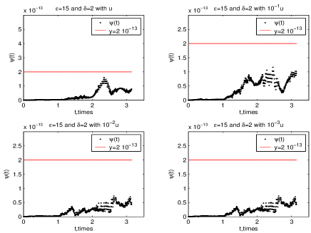
  Figure 4: Comparisons of two solutions

  In this latter example, the unperturbed system is unstable and the rank one perturbation systems remain unstable when the vector $u\in\left\{u,10^{-1}u,10^{-2}u,10^{-3}\right\}$. This justifies the existence of a neighborhood of the unperturbed system in which any rank one perturbation of the system is unstable.

6 Conclusion

From a theory developed by C. Mehl, et al., on the rank one perturbation of symplectic matrices (see [13]), we defined the rank one perturbation of Hamiltonian system of periodic coefficients. After an adaptation of some results of [13] on symplectic matrices when they depend on a time parameter, we show that the rank one perturbation of the fundamental solution of a Hamiltonian system with periodic coefficients is solution of the rank one perturbation of the system. A result of this theory, we give a consequence of the strong stability on a small rank one perturbation of these Hamiltonian systems. Two numerical examples are given to illustrate this theory.

In future work, we will look how to use the rank one perturbation of Hamiltonian system with periodic coefficients to analyze the behavior of their multipliers and also how this theory can analyze their strong stability ?

References:

• [1] C. Brezinski, Computational Aspercts of Linear Control, Kluwer Academic Publishers, 2002.
• [2] M. Dosso, Sur quelques algorithms d’analyse de stabilit forte de matrices symplectiques, PHD Thesis (September 2006), Universit de Bretagne Occidentale. Ecole Doctorale SMIS, Laboratoire de Math matiques, UFR Sciences et Techniques.
• [3] M. Dosso, N. Coulibaly, An Analysis of the Behavior of Mulpliers of Hamiltonian System with periodic. Far East Journal of Mathematical Sciences. Vol. 99, Number 3, 2016, 301–322.
• [4] M. Dosso, N. Coulibaly, Symplectic matrices and strong stability of Hamiltonian systems with periodic coefficients. Journal of Mathematical Sciences : Advances and Applications. Vol. 28, 2014, Pages  15–38.
• [5] M. Dosso, N. Coulibaly and L. Samassi, Strong stability of symplectic matrices using a spectral dichotomy method. Far East Journal of Applied Mathematics. Vol. 79, Number 2, 2013, pp. 73–110.
• [6] M. Dosso and M. Sadkane. On the strong stability of symplectic matrices. Numerical Linear Algebra with Applications, 20(2) (2013), 234–249.
• [7] M. Dosso, M. Sadkane, A spectral trichotomy method for symplectic matrices, Numer Algor. 52(2009), 187–212
• [8] S.K. Godunov, Verification of boundedness for the powers of symplectic matrices with the help of averaging, Siber. Math. J. 33,(1992),  939–949.
• [9] S.K. Godunov, M. Sadkane, Numerical determination of a canonical form of a symplectic matrix, Siberian Math. J. 42(2001), 629–647.
• [10] S.K. Godunov, M. Sadkane, Spectral analysis of symplectic matrices with application to the theory of parametric resonance, SIAM J. Matrix Anal. Appl. 28(2006), 1083–1096.
• [11] B. Hassibi, A. H. Sayed, T. Kailath, Indefinite-Quadratic Estimation and Control, SIAM, Philadelphia, PA, 1999.
• [12] P. Lancaster, L. Rodman, Algebraic Riccati Equations, Clarendon Press, 1995.
• [13] C. Mehl, V. Mehrmann, A.C.M. Ran, and L. Rodman. Eigenvalue perturbation theory under generic rank one perturbations: Symplectic, orthogonal, and unitary matrices. BIT, 54(2014), 219–255.
• [14] C. Mehl, V. Mehrmann, A.C.M. Ran and L. Rodman. Eigenvalue perturbation theory of classes of structured matrices under generic structured rank one perturbations. Linear Algebra Appl., 435(2011), 687–716.
• [15] V.A., Yakubovich, V.M. Starzhinskii, Linear differential equations with periodic coefficients, Vol. 1 & 2., Wiley, New York (1975)
• [16] YAN Qing-you. The properties of a kind of random symplectic matrices. Applied mathematics and Mechanics. Vol 23, No 5, May 2002.