Property trends in simple metals: an empirical potential approach

Abstract

We demonstrate that the melting points and other thermodynamic quantities of the alkali metals can be calculated based on static crystalline properties. To do this we derive analytic interatomic potentials for the alkali metals fitted precisely to cohesive and vacancy energies, elastic moduli, lattice parameter and crystal stability. These potentials are then used to calculate melting points by simulating the equilibration of solid and liquid samples in thermal contact at ambient pressure. With the exception of lithium, remarkably good agreement is found with experimental values. The instability of the bcc structure in Li and Na at low temperatures is also reproduced, and, unusually, is not due to a soft T1N phonon mode. No forces or finite temperature properties are included in the fit, so this demonstrates a surprisingly high level of intrinsic transferrability in the simple potentials. Currently, there are few potentials available for the alkali metals, so in addition to demonstrating trends in behaviour, we expect that the potentials will be of broad general use.

I Introduction

The thermodynamic properties of Group 1A metals vary systematically down the group. Cohesive energies and elastic constants decrease from Li-Cs, while lattice parameters increase. This makes them an ideal testground for testing thermodynamic relationships between solid properties and melting points.

Melting points are impossible to calculate analytically, and it is well known that different parameterizations of metal potentials can give very different results for calculated melting points. Thus to examine trends down a group, we require an analytic description of interatomic interactions. This means creating an interatomic potential fully specified by a small number of materials properties.

We wish to derive a family of interatomic potentials describing the alkali metals which can be used in classical molecular dynamics. To ensure comparability, we aim for a form with a minimal number of parameters, fully determined by the fitting data. We choose to use the simplest form which describes many-body metallic interactions, the second-moment approximation to tight bindingDucastelle and Cyrot-Lackmann (1970); Finnis and Sinclair (1984). The motivation for this theory comes from the idea of a local density of states projected onto an atom, but the actual potentials are similar in form to the embedded atom methodDaw and Baskes (1984) (EAM). This is based on the conceptual idea of embedding an atom into a preexisting charge density, and calculating the energy change.

In either case the energy is written as:

$$\mathcal{U}=\sum_{i}{F({\rho}_{i})}+\frac{1}{2}\sum_{i,j\neq i}{{V}_{ij}(r_{ij})}$$ (1)

with

$${\rho}_{i}=\sum_{j\neq i}{\phi_{ij}(r_{ij})}$$ (2)

For elements where binding comes from a single band, the second-moment approach to second moment potentials gives $F=\sqrt{}$, although for materials where binding comes from two bands this is more complicatedAckland and Reed (2003); Ackland (2006). For alloys, another subtle difference arises. In EAM $\phi_{ij}$ is interpreted as the charge density due to atom $j$, such that $\phi_{ij}=\phi_{j}\neq\phi_{ji}$, while in the tight binding picture it represents a hopping integral, and $\phi_{ij}=\phi_{ji}$.

The second moment approximation does not account for the shape or filling of the band, this is implicit in the parameterization. Consequently, to examine trends in behavior, we should consider materials with similar band shapes and band fillings. It appears that the alkali metals provide an ideal case where this will work well: they have simple half-filled $s$-band binding and minimal $s-d$ and $s-p$ hybridization.

Parameterization of potential models can follow two paths: maximal or minimum fitting parameters. In the first case, one tries to achieve the most highly tuned potential by fitting to as many known properties as possible. This gives the best possible description of a particular material. In the second, used here, one uses a minimal set of fitting data. Such potentials may not reproduce materials properties as successfully, but if they do for a whole group of materials, it demonstrates transferrability due to the physics, and a physical connection between the fitted and unfitted properties. Furthermore, simple potentials should be treated as a null hypothesis, and a systematic failure to predict properties indicates missing physics, even if the properties can be reproduced by judicious fitting. For example, we see later that neglect of zero-point effects in Lithium increases the calculated melting point.

Our main aim is to ensure comparability between the metals, rather than transferability of a particular potential. Consequently, we consciously eschew approaches such as MEAMBaskes (1992), two-bandAckland and Reed (2003) and REAMZhou and Huang (2013) which have added complexity which gives the possibility to fit more closely to experimental data. We also avoid overconstrained data fitting which would allow tuning to a particular elementBrommer and Gähler (2007). Without doubt, additional fitting parameters could be used to “tune” melting points, phase transitions, or other properties of interest, but our interest here is the intrinsic transferability of the potentials.

II Calculations

II.1 Alkali Metals and Periodicity

The alkali metals comprise the group I elements excluding Hydrogen. They are particularly soft metals with low melting points and all adopt a body-centered cubic (bcc) crystal structure at standard temperature and pressure. Their bcc lattice parameters are notably large, resulting in low densities and high compressibilities. Being group I elements they have a [noble gas] + ns¹ electronic structure and have been studied extensively as a test of theories of ‘simple’ metals.

The solid/liquid phase transition in various metals has been studied using both classical and quantum mechanical methods and with both Monte Carlo and Molecular Dynamics approaches. Many-body potentials for one-off alkali metals have been created beforeWilson et al. (2015); Vella et al. (2014); Belashchenko (2012); Ouyang et al. (1994), but they have problems with crystal stability and have not yet been applied by other groups. Typical discrepancies between experimental and simulated melting points are on the order of hundreds of degrees.Mendelev and Ackland (2007)

The functions $\phi$ and $V$ were defined as cubic splines $F$ is given by its Finnis-SinclairFinnis and Sinclair (1984) form ($F={\rho}^{1/2}$) and

$$V(r)=\sum_{k=1}^{6}{a_{k}{(r_{k}-r)}^{3}}H(r_{k}-r)$$ (3)

$$\phi(r)=\sum_{k=1}^{2}{A_{k}{(R_{k}-r)}^{3}}H(R_{k}-r)$$ (4)

where $H(x)$ is the Heaviside step function: $H(x)=0$ for $x<0$ and $H(x)=1$ for $x>0$.

The spline knot points ($r_{k}$ and $R_{k}$) are not treated as adjustable parameters, their values were taken from previous workHan et al. (2003), scaled by the lattice parameter to give a potential extending to second neighbours. The 7 parameters $a_{k}$ and $A_{k}$ were chosen to exactly fit target values for cohesive energy, lattice constant, three elastic constants, unrelaxed vacancy formation energy and fcc-bcc energy difference (Table 1). These properties are independent of the final parameter $a_{6}$, which controls the short ranged repulsion inside the perfect crystal nearest neighbour distance. This was set to a constant value across all potentials, scaled by the cubed lattice parameter. The $r_{k}$ parameters were set to be the same for all elements, as a fraction of lattice parameter (see Table 2).

It can be noticed that all energies and elastic moduli systematically decrease down the period, by factors of about 2 and 6 respectively. However, the reduction in the elastic moduli is almost entirely due to the increased lattice parameter: the elastic moduli in units of eV per unit cell volume are remarkably constant.

Element	$a_{0}$	C11	C12	C44	$E_{coh}$	$E_{vac}$	$E_{fcc}$
Li	3.51	0.092	0.078	0.067	1.648	0.54	-0.006
Na	4.2906	0.0512	0.0418	0.0345	1.109	0.35	-0.003
K	5.328	0.0260	0.0213	0.0179	0.923	0.308	+0.001
Rb	5.585	0.0213	0.0179	0.0138	0.840	0.28	+0.012
Cs	6.141	0.0162	0.0135	0.00999	0.788	0.263	+0.016

Table 1: Fitting Data: bcc lattice parameter (Å), elastic constants (eV/ų) cohesive energy, unrelaxed vacancy formation energy and fcc energy per atom (eV) above the bcc value. For sodium the low temperature ground state is actually fcc, and for lithium it is reported to be a 9R complex close-packed structure, however bcc is stable at room temperature, and we fit to the bcc properties

The square root dependence appears to make the fitting nonlinear, however this nonlinearity can be transferred from the fitting to the data being fitted. Specifically, the many-body term’s parameters $A_{k}$ can be fully determined by linear fit to two quantities which are explicitly zero for any pair potential, i.e.

• the difference between vacancy formation energy and cohesive energy $(E_{coh}-E_{vac})$

• the Cauchy Pressure $C_{12}-C_{44}$

The pair-potential parameters $a_{i}$ can then be determined by a linear fit to the difference between the required property and the contribution from the many-body term. The lattice parameter is fitted by setting the derivative of the energy to zero at the required value. The fitting problem is then reduced to a simple 7x7 matrix problem.

We also attempted the fit using a genetic algorithmDieterich and Hartke (2010), which converged immediately for the linearly transformed problem, but failed to find the known solution within required several weeks of CPU time when fitting the seven pieces of data directly. The algorithm got “stuck” in many local minima, all of which are eliminated by transforming the fitting problem to linear algebra.

For meaningful comparison, it is useful that the linear fit for all potentials gives a broadly similar solution: parameters are given in Table 2. The best way to visualize these potentials is the “effective pair potential”, which incorporates both attractive and repulsive parts, approximating $\rho$ by its equilibrium value at the minimum bcc energy $\rho_{0}$.

$$V_{eff}(r)=V(r)+\phi(r)/\rho_{0}$$ (5)

These functions $V_{eff}(r)$ shown in Fig. 1. Several trends are notable here, the most obvious being the range and depth of the potentials. More subtle is the development of a secondary minimum in Li, Na and K. Although the parameterization data comes from bcc only, this feature is ultimately responsible for the stability of fcc in Li and Na at low temperature, and K at high pressure. The existence of such a minimum is not explicit in the second moment approach. If it appeared for a single material, we might have dismissed it as a fitting anomaly. However, it is tempting to speculate that it arises from a mismatch between the optimal electron density and the first minimum in the screened electrostatic potential. This latter emerges from the free electron theory, the oscillations ultimately being related to the Fermi wavevectorAnimalu and Heine (1965).

Li
$a_{k}$	-9.741070	52.683696	-75.033831	39.542714	-14.782577	3.079201
$A_{k}$	20.537818	-34.233934
$l.p.$	3.510000
Na
$a_{k}$	-4.194182	27.427457	-44.559331	31.771667	-15.792378	3.079201
$A_{k}$	8.719427	-13.899855
$l.p.$	4.290600
K
$a_{k}$	-1.723040	5.203775	4.914958	-21.814488	20.037488	3.079201
$A_{k}$	5.438419	-8.619811
$l.p.$	5.328000
Rb
$a_{k}$	-2.924102	15.101598	-19.036044	8.221297	1.000245	3.079201
$A_{k}$	4.151321	-6.163082
$l.p.$	5.585000
Cs
$a_{k}$	-2.184268	9.803950	-8.445145	-2.009154	8.266863	3.079201
$A_{k}$	3.415288	-4.866591
$l.p.$	6.141000
$r_{k}$	1.3	1.22	1.15	1.06	0.95	$\sqrt{3/4}$
$R_{k}$	1.3	1.2

Table 2: Tabulated parameters for the alkali metal potentials. For ease of comparison, values are scaled by the lattice parameter (l.p.), such that the units are eV per lattice parameter cubed. This enables up to use consistent values for $R_{i}$ and $r_{i}$, enhancing comparability of the potentials

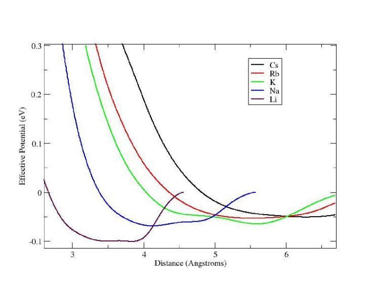
Figure 1: Effective pairwise potentials (table 3) showing trends down the group.

Element		$\mathbf{T_{m}^{exp}\,/\,K}$	$\mathbf{T_{m}^{sim}\,/\,K}$	$\mathbf{\Delta\,h\,/\,kJ\,mol^{-1}}$	$\mathbf{\Delta\,v\,/\,mL\,mol^{-1}}$
Lithium	Li	454	660(2)	44.38(1)	0.0301(2)
Sodium	Na	370	411(2)	3.51(2)	0.223(3)
Potassium	K	336	344(2)	2.99(2)	0.211(1)
Rubidium	Rb	312	333(2)	2.70(2)	1.385(1)
Caesium	Cs	301	305(2)	2.60(2)	1.957(1)

Table 3: Tabulated results for the alkali metal potentials. Shown are the experimental and simulated melting points, as well as the specific enthalpy and volume differences between the solid and liquid phases at the coexistence temperature.

II.2 Simulating Phase Transitions

To calculate the melting point, we employ the coexistence methodMorris et al. (1994) in which pre-formed samples of the two phases are brought together and allowed to equilibrate. A solid/liquid interface is present at the start of the simulation and the particle velocities are initialized to approximate the anticipated coexistence temperature. The total enthalpy of the system is held constant, in an NPE ensemble, so that if the initial temperature is below (above) $T_{m}$ the phase boundary will move and some of the sample will freeze (melt). The “ringing mode” is eliminated in an initial equilibration phase by setting the first time derivatives of the Nose and Parrinello-Rahman extended Lagrangian parameters to zero whenever their sign differs from the second derivative. This algorithm does not correspond to any Lagrangian, but very efficiently removes energy from ringing modes. After a short equilibration period, when the energy in the fictitious dynamic modes approaches kT, we continue production runs with the standard NPE Lagrangian. This process proved necessary because of the poor coupling between the fictitious degrees of freedom and the rest of the system. We note that the same ringing behaviour is present in the NVE ensemble, manifesting itself as an oscillation in the internal pressure.

On a timescale much longer than the ringing mode equilibration, the latent heat released during the transition increases (decreases) the temperature of the sample until it reaches $T_{m}$. We used a supercell with 17576 atoms (initialized with 8788 atoms of bcc: $13\times 13\times 26$, and a similar amount of melt). Convergence was checked by comparing several runs initialising the temperature above and below the expected melt point, and observing that in each case the simulation went to the same final temperature. The final configurations were visualized using VMD Humphrey et al. (1996) to verify that both crystal and solid phases were still present (Fig 2, inset).

All calculations reported here were carried out using the MOLDY molecular dynamics packageAckland et al. (2011). The potentials were also converted to LAMMPS formatPlimpton (1995) and are available at the NIST potential databaseBecker et al. (2013). These versions have adjustments at very short range to fit to the Biersack-ZieglerBiersack and Ziegler (1982) functions which are popular in radiation damage studies, but give identical results for the problems considered here.

Figure 2 shows the changes in temperature for three constant-energy simulations of a potassium supercell. Convergence times depend primarily on the atomic mass and on the system size and were typically on the order of hundreds of picoseconds.

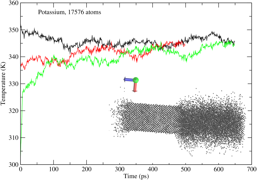
Figure 2: Temperature evolution of coexisting crystalline and liquid K in the NPEp ensemble. Simulations had temperatures initialized above or below. After relaxation all systems equilibrated to a single coexistence temperature. Inset is a snapshot of the simulation, with the periodic boundary conditions removed in the graphics to show the two distinct phases. Similar behaviour was observed for other elements

The thermal expansion of the materials was also calculated by constant pressure heating simulations (Fig 3). Thermal expansion depends on third derivatives of the potentials, which are not fitted, nevertheless, both the values and trends across the group are in good agreement with experiment. There is a weak temperature dependence, and in the absence of quantization of the phonons, calculated thermal expansions remain finite to 0K. The heating calculations also showed melting transitions in all elements, and a martensitic transformation to a faulted close-packed structure at low-T in Li and Na, also in accord with experiment. We observe that although this is an excellent test of phase stability, “heat until it transforms” is not a reliable way to determine transition temperatures.

II.3 Phase Coexistence Lines at pressure

In order to generate coexistence lines on the PT phase diagram of the alkali metals the Clausius-Clapeyron equation was integrated using a fourth order predictor-corrector algorithm. The coexistence conditions ($P$,$T$) were extrapolated over a range of several hundred degrees in intervals of 0.01 K. Shown in Figure 4 are the results for sodium, others being similar.

At high pressure, the alkali metals are known to exhibit a maximum in the melting curve. It is striking that none of the potentials presented here exhibits this feature: this tells us that physics beyond that sampled in the ambient pressure state, where the fitting was done, will be required. Another high pressure phenomenon, transformation to fcc, was observed in all the potentials, as a consequence of the lower bulk modulus and higher packing density under pressure. In Na, and Li, there is a martensitic transition to a complex close-packed structure at low temperaturesVaks et al. (1989); Hanfland et al. (2002)

II.4 Phonons

Phonon spectra can be calculated by lattice dynamics using the analytic second derivatives of the potential. For bcc, the symmetry constraints and fit to elastic constants mean that agreement with experiment is exact for the slope at the $\Gamma$ point, so the general similarity with neutron data is unsurprising and trends across the group can be readily seen. It is notable that Li and Na, which are unstable with respect to fcc at low temperature, have stable bcc phonon spectra, unlike other elements such as Ti and Zr, which are calculated to have negative bcc shear moduli at 0KMacLeod et al. (2012); Pinsook and Ackland (1999); Mendelev and Ackland (2007), and transform to bcc at high temperatures due to soft T1N modes. Figures 5 and 6 show phonon spectra for Li and Cs, other elements being similar (Supplemental Figure 3). The stable phases have real phonons throughout, but notably, fcc Cs is mechanically unstable with imaginary phonon modes along $\Gamma-L$. At higher pressures when Cs becomes thermodynamically stable, all phonons are stable.

It is also noticeable that the phonon frequencies are higher in fcc than in bcc. This has the effect of stabilizing the bcc phase at higher temperatures. It is notable that this feature is present in all cases, despite the properties of fcc elements being excluded from the fitting process.

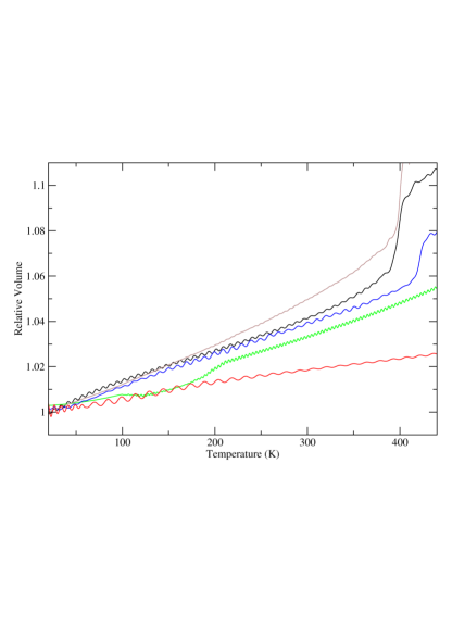
Figure 3: Volume against temperature for steady heating in NPT molecular dynamics. Volumes are scaled to their low-T bcc value to show trends in thermal expansion across the group, from lowest to highest Li (red) Na (green) K (blue) Rb (black) and Cs (brown). Heating rate was 1 K per 4000 timesteps, the timestep varying with the atomic mass from 0.1fs for Li to 1fs for Cs. Ringing-mode volume oscillations come from the Nose thermostat and Parrinello-Rahman barostat and persist for hundreds of picosecond. Sharp rises in volume around 400K for Cs, Rb, K, indicate melting, although hysteresis means this is not the thermodynamic melting point. The large oscillations for Li show the immediate transformation to close-packing at low T. The two changes in slope for Na come from the (metastable)bcc-fcc transition at about 100K, and the subsequent fcc-bcc retransformation around 200K.

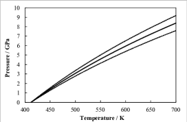
Figure 4: Coexistence line for Na integrated from a single simulation at $P=0.0$ using the Clausius-Clapeyron equation. Solid Line: Best estimate based on the specific enthalpy and volume differences between the solid and liquid at the zero-pressure melting point of 405 K. Dashed Lines: 67% confidence intervals based on the relative errors in the initial slope.

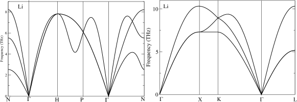
Figure 5: Phonon spectra calculated using lattice dynamics in lithium in bcc (left, fitted) and fcc (right).

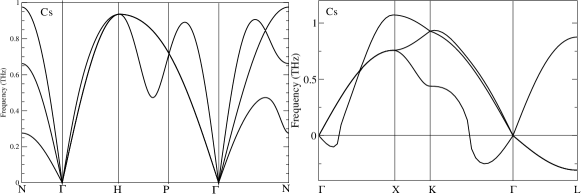
Figure 6: Phonon spectra calculated using lattice dynamics in Cs bcc (left, as fitted) and fcc (unstable phase).

Coexistence lines for the remaining alkali metals are shown in supplemental materials.

II.5 Parameter sensitivity

Our fitting process is fully defined, however there are uncertainties in the quantities being fitted. We tested the melting points against variation of the fitting parameters for lithium, and it proved to be remarkably robust except with respect to the short-range part of the repulsion (inside 3.03975$\AA$, parameter $a_{6}$), which is uncorrelated with the fitting data and chosen to match smoothly to the Biersack-ZieglerBiersack and Ziegler (1982) functions. Stiffer short range repulsion accords to higher melting point (and thermal expansion). We speculate that this is because the steep repulsion reduces the available phase space for the liquid state by more than the solid, reducing its relative entropic advantage. It is possible to lower the melting point by up to 100K before other unreasonable behaviour appears - notably that the liquid density becomes lower than the solid and the thermal expansivity becomes negative.

The very good agreement elsewhere suggests that for lithium our model is missing some physics. A reasonable candidate is the nuclear quantum effects, which are especially important for low mass effects. The classical molecular dynamics does not include the zero-point energy (ZPE) of lithium, which we calculated in our lattice dynamics and by using the CASTEP density functional packageCASTEP to be around 39meV/atom, corresponding to a Debye temperature of around 450K, somewhat higher than a previous studymoruzzi. ZPE dominates the vibrational contribution to the free energy below the Debye Temperature, which in lithium is close to the melting point. The effect on the melting point is that the quantum vibrational entropy is about half the classical value, and must therefore be assumed to be significant. The solid lithium ZPE is also significantly larger than the latent heat of melting (13meV/atom), which indicates that the liquid ZPE is also significant.

An accurate assessment of nuclear quantum effects on the melting point would require evaluating the ZPE for the liquid, for which there is no suitable theory. Qualitatively, we can expect that the zero point energy of the solid will be greater than that of the liquid, since the liquid has no resistance to shear. Consequently, nuclear quantum effects will destabilize the solid compared to the liquid, lowering the melting point. This is consistent with our observation that our calculated classical melting point is too high.

III Discussion and Conclusions

We have derived a series of analytic many-body interatomic potentials which describe the simple metals. Although the potentials are fitted only to crystal properties, they give a good description of the melting point with the notable exception of lithium, which we ascribe to nuclear quantum effects ignored in our MD.

The potentials are fitted to fcc and bcc energy at 0K, and to properties of bcc at ambient conditions, Consequently, the transition into a higher temperature bcc state in Li and Rb is a successful prediction. It is due to the lower phonon frequencies in bcc: the only contributory factor which was fitted is the bcc elasticity tensor. Heuristically, the fcc stability can be attributed to the appearance of a secondary minimum in the effective potential, which is more pronounced in the lower Z-elements. This minimum is not an input to the theory, it emerges from the fitting process, implying that its existence manifests in some feature of the fitted bcc elasticity.

Overall, the work shows that a number of trends can be deduced from minimal fitted data. Essentially, the input is that energies and elastic moduli are lower for higher-Z elements, while lattice parameters are larger. From this we deduce that the thermal expansion and volume change on melting increases down the group, while the melting point is reduced.

III.1 Acknowledgements

We thank The University of Edinburgh for the CPU time allocation, EPSRC for support under EP/F010680/1. Open data for the potentials in this paper is available at http://www.ctcms.nist.gov/potentials/

References

- Ducastelle and Cyrot-Lackmann (1970) F. Ducastelle and F. Cyrot-Lackmann, Journal of Physics and Chemistry of Solids 31, 1295 (1970).
- Finnis and Sinclair (1984) M. Finnis and J. Sinclair, Philosophical Magazine A 50, 45 (1984).
- Daw and Baskes (1984) M. S. Daw and M. I. Baskes, Physical Review B 29, 6443 (1984).
- Ackland and Reed (2003) G. J. Ackland and S. K. Reed, Physical Review B 67, 174108 (2003).
- Ackland (2006) G. J. Ackland, Journal of Nuclear Materials 351, 20 (2006).
- Baskes (1992) M. Baskes, Physical Review B 46, 2727 (1992).
- Zhou and Huang (2013) L. Zhou and H. Huang, Physical Review B 87, 045431 (2013).
- Brommer and Gähler (2007) P. Brommer and F. Gähler, Modelling and Simulation in Materials Science and Engineering 15, 295 (2007).
- Wilson et al. (2015) S. Wilson, K. Gunawardana, and M. Mendelev, The Journal of Chemical Physics 142, 134705 (2015).
- Belashchenko (2012) D. Belashchenko, Inorganic Materials 48, 79 (2012).
- Ouyang et al. (1994) Y.-F. Ouyang, B.-W. Zhang, S.-Z. Liao, et al., Science in China series A 37, 1232 (1994).
- Vella et al. (2014) J. R. Vella, F. H. Stillinger, A. Z. Panagiotopoulos, and P. G. Debenedetti, The Journal of Physical Chemistry B (2014).
- Mendelev and Ackland (2007) M. I. Mendelev and G. J. Ackland, Philosophical Magazine Letters 87, 349 (2007).
- Han et al. (2003) S. Han, L. A. Zepeda-Ruiz, G. J. Ackland, R. Car, and D. J. Srolovitz, Journal of applied physics 93, 3328 (2003).
- Dieterich and Hartke (2010) J. M. Dieterich and B. Hartke, Molecular Physics 108, 279 (2010).
- Animalu and Heine (1965) A. O. Animalu and V. Heine, Philosophical Magazine 12, 1249 (1965), URL http://dx.doi.org/10.1080/14786436508228674.
- Morris et al. (1994) J. R. Morris, C. Z. Wang, K. M. Ho, and C. T. Chan, Phys. Rev. B 49, 3109 (1994), URL http://link.aps.org/doi/10.1103/PhysRevB.49.3109.
- Humphrey et al. (1996) W. Humphrey, A. Dalke, and K. Schulten, Journal of molecular graphics 14, 33 (1996).
- Ackland et al. (2011) G. J. Ackland, K. D’Mellow, S. L. Daraszewicz, D. J. Hepburn, M. Uhrin, and K. Stratford, Computer Physics Communications 182, 2587 (2011).
- Plimpton (1995) S. Plimpton, Journal of Computational Physics 117, 1 (1995).
- Becker et al. (2013) C. A. Becker, F. Tavazza, Z. T. Trautt, and R. A. B. de Macedo, Current Opinion in Solid State and Materials Science 17, 277 (2013).
- Biersack and Ziegler (1982) J. Biersack and J. Ziegler, Nucl. Instrum. Methods 194, 93 (1982).
- Vaks et al. (1989) V. G. Vaks, M. I. Katsnelson, V. G. Koreshkov, A. I. Likhtenstein, O. E. Parfenov, V. F. Skok, V. A. Sukhoparov, A. V. Trefilov, and A. A. Chernyshov, Journal of Physics: Condensed Matter 1, 5319 (1989), URL http://stacks.iop.org/0953-8984/1/i=32/a=001.
- Hanfland et al. (2002) M. Hanfland, I. Loa, and K. Syassen, Phys. Rev. B 65, 184109 (2002), URL http://link.aps.org/doi/10.1103/PhysRevB.65.184109.
- MacLeod et al. (2012) S. G. MacLeod, B. E. Tegner, H. Cynn, W. J. Evans, J. E. Proctor, M. I. McMahon, and G. J. Ackland, Phys. Rev. B 85, 224202 (2012), URL http://link.aps.org/doi/10.1103/PhysRevB.85.224202.
- Pinsook and Ackland (1999) U. Pinsook and G. J. Ackland, Physical Review B 59, 13642 (1999).