eHDG: An Exponentially Convergent Iterative Solver for HDG Discretizations of Hyperbolic Partial Differential Equations.

Abstract

We present a scalable and efficient iterative solver for high-order hybridized discontinuous Galerkin (HDG) discretizations of hyperbolic partial differential equations. It is an interplay between domain decomposition methods and HDG discretizations. In particular, the method is a fixed-point approach that requires only independent element-by-element local solves in each iteration. As such, it is well-suited for current and future computing systems with massive concurrencies. We rigorously show that the proposed method is exponentially convergent in the number of iterations for transport and linearized shallow water equations. Furthermore, the convergence is independent of the solution order. Various 2D and 3D numerical results for steady and time-dependent problems are presented to verify our theoretical findings.

1 Introduction

The discontinuous Galerkin (DG) method was originally developed by Reed and Hill [33] for the neutron transport equation, first analyzed in [22, 20], and then has been extended to other problems governed by partial differential equations (PDEs) [11]. Roughly speaking, DG combines advantages of classical finite volume and finite element methods. In particular, it has the ability to treat solutions with large gradients including shocks, it provides the flexibility to deal with complex geometries, and it is highly parallelizable due to its compact stencil. As such, it has been adopted, for example, to solve large-scale forward [2, 35] and inverse [6] problems. However, for steady state problems or time-dependent ones that require implicit time-integrators, DG methods typically have many more (coupled) unknowns compared to the other existing numerical methods, and hence more expensive in general.

In order to mitigate the computational expense associated with DG methods, Cockburn, coauthors, and others have introduced hybridizable (also known as hybridized) discontinuous Galerkin (HDG) methods for various types of PDEs including Poisson-type equation [9, 10, 21, 28, 7, 13], Stokes equation [8, 29], Euler and Navier-Stokes equations, wave equations [32, 27, 31, 23, 30, 17, 12], to name a few. The upwind HDG framework proposed in [3, 4, 5] provides a unified and a systematic construction of HDG methods for a large class of PDEs. In HDG discretizations, the coupled unknowns are single-valued traces introduced on the mesh skeleton, i.e. the faces, and the resulting matrix is substantially smaller and sparser compared to standard DG approaches. Once they are solved for, the usual DG unknowns can be recovered in an element-by-element fashion, completely independent of each other. Nevertheless, the trace system is still a bottleneck for practically large-scale applications, where complex and high-fidelity simulations involving features with a large range of spatial and temporal scales are necessary.

Meanwhile, Schwarz-type domain decomposition methods (DDMs) have been introduced as procedures to parallelize and solve partial differential equations numerically, where each iteration involves the solutions of the original equations on smaller subdomains [24, 25, 26]. Among the many DDMs, Schwarz waveform relaxation methods and optimized Schwarz methods [18, 1, 19, 14, 15, 34], have attracted substantial attention over the past decade since they can be adapted to the physics of the underlying problems and thus lead to very efficient parallel solvers for challenging problems. We view the HDG method as an extreme DDM approach in which each subdomain is an element.

While either HDG community or DDM community can contribute individually towards advancing its own field, the potential for a true breakthrough may lie in bringing together the advances from both sides and in exploiting opportunities at their interfaces. In this paper, we blend the HDG method and optimized Schwarz idea to produce a efficient and scalable iterative approach for HDG methods. One of the main features of the proposed approach is that it has exponential convergence rate, and for that reason we term it as eHDG. The method can be viewed as a fixed-point approach that requires only independent element-by-element local solves in each iteration. As such, it is well-suited for current and future computing systems with massive concurrencies. We rigorously show that the proposed method is exponentially convergent in the number of iterations for transport and linearized shallow water equations. Furthermore, the convergence is independent of the solution order. The theoretical findings will be verified on various 2D and 3D numerical results for steady and time-dependent problems.

Let us mention that in [15], Schwarz methods for the hybridizable interior penalty (IPH) method have also been introduced. The methods have been proposed entirely at the discrete level and thus holds for arbitrary interfaces between two subdomains. It is proved that for an arbitrary two-subdomain decomposition the Schwarz algorithms have a convergence factor $1-O(h)$, and $1-O(\sqrt{h}),$ which means the algorithms converge slower and slower when we refine the mesh.

2 Notations for HDG discretizations

In this section we introduce common notations and conventions to be used in the following sections where we propose and rigorously analyze the eHDG approach for scalar and systems of hyperbolic PDEs in both steady and time-dependent cases. Let us partition an open and bounded domain $\Omega\in{\mathbb{R}}^{d}$ into ${N_{\text{el}}}$ non-overlapping elements ${K_{j}},j=1,\ldots,{N_{\text{el}}}$ with Lipschitz boundaries such that $\Omega_{h}:=\cup_{j=1}^{N_{\text{el}}}{K_{j}}$ and $\overline{\Omega}=\overline{\Omega}_{h}$. Here, $h$ is defined as $h:=\max_{j\in\left\{1,\ldots,{N_{\text{el}}}\right\}}diam\left({K_{j}}\right)$. We denote the skeleton of the mesh by ${\mathcal{E}_{h}}:=\cup_{j=1}^{N_{\text{el}}}\partial K_{j}$, the set of all (uniquely defined) faces $e$. We conventionally identify $\mathbf{n}^{-}$ as the normal vector on the boundary ${\partial K}$ of element $K$ (also denoted as $K^{-}$) and $\mathbf{n}^{+}=-\mathbf{n}^{-}$ as the normal vector of the boundary of a neighboring element (also denoted as $K^{+}$). Furthermore, we use $\mathbf{n}$ to denote either $\mathbf{n}^{-}$ or $\mathbf{n}^{+}$ in an expression that is valid for both cases, and this convention is also used for other quantities (restricted) on a face $e\in{\mathcal{E}_{h}}$.

For simplicity in writing we define $\left(\cdot,\cdot\right)_{K}$ as the $L^{2}$-inner product on a domain $K\in{\mathbb{R}}^{d}$ and $\left<\cdot,\cdot\right>_{K}$ as the $L^{2}$-inner product on a domain $K$ if $K\in{\mathbb{R}}^{{d}-1}$. We shall use $\left\|\cdot\right\|_{K}:=\left\|\cdot\right\|_{{L^{2}\left(K\right)}}$ as the induced norm for both cases and the particular value of $K$ in a context will indicate which inner product the norm is coming from. We also denote the ${\varepsilon}$-weighted norm of a function $u$ as $\left\|u\right\|_{{\varepsilon},K}:=\left\|\sqrt{{\varepsilon}}u\right\|_{K}$ for any positive ${\varepsilon}$. We shall use boldface lowercase letters for vector-valued functions and in that case the inner product is defined as $\left(\mathbf{u},\mathbf{v}\right)_{K}:=\sum_{i=1}^{m}\left(\mathbf{u}_{i},\mathbf{v}_{i}\right)_{K}$, and similarly $\left<\mathbf{u},\mathbf{v}\right>_{K}:=\sum_{i=1}^{m}\left<\mathbf{u}_{i},\mathbf{v}_{i}\right>_{K}$, where ${m}$ is the number of components ($\mathbf{u}_{i},i=1,\ldots,{m}$) of $\mathbf{u}$. Moreover, we define $\left(\mathbf{u},\mathbf{v}\right)_{\Omega}:=\sum_{K\in\Omega_{h}}\left(\mathbf{u},\mathbf{v}\right)_{K}$ and $\left<\mathbf{u},\mathbf{v}\right>_{\mathcal{E}_{h}}:=\sum_{e\in{\mathcal{E}_{h}}}\left<\mathbf{u},\mathbf{v}\right>_{e}$ whose induced (weighted) norms are clear, and hence their definitions are omitted. We employ boldface uppercase letters, e.g. $\mathbf{L}$, to denote matrices and tensors. In addition, subscripts are used to denote the components of vectors, matrices, and tensors.

We define ${\mathcal{P}}^{p}\left(K\right)$ as the space of polynomials of degree at most ${p}$ on a domain $K$. Next, we introduce two discontinuous piecewise polynomial spaces

$${{\mathbf{V}}_{h}}\left(\Omega_{h}\right) :=\left\{\mathbf{v}\in\left[L^{2}\left(\Omega_{h}\right)\right]^{2}:\left.\mathbf{v}\right\rvert_{K}\in\left[{\mathcal{P}}^{p}\left(K\right)\right]^{2},\forall K\in\Omega_{h}\right\},$$

$${\boldsymbol{\Lambda}_{h}}\left({\mathcal{E}_{h}}\right) :=\left\{\boldsymbol{\lambda}\in\left[{L^{2}\left({\mathcal{E}_{h}}\right)}\right]^{2}:\left.\boldsymbol{\lambda}\right\rvert_{e}\in\left[{\mathcal{P}}^{p}\left(e\right)\right]^{2},\forall e\in{\mathcal{E}_{h}}\right\},$$

and similar spaces for ${{\mathbf{V}}_{h}\left(K\right)}$ and ${\boldsymbol{\Lambda}_{h}\left(e\right)}$ by replacing $\Omega_{h}$ with $K$ and ${\mathcal{E}_{h}}$ with $e$. For scalar-valued functions, we denote the corresponding spaces as

$${{V}_{h}}\left(\Omega_{h}\right) :=\left\{v\in L^{2}\left(\Omega_{h}\right):\left.v\right\rvert_{K}\in{\mathcal{P}}^{p}\left(K\right),\forall K\in\Omega_{h}\right\},$$

$${{\Lambda}_{h}}\left({\mathcal{E}_{h}}\right) :=\left\{\lambda\in{L^{2}\left({\mathcal{E}_{h}}\right)}:\left.\lambda\right\rvert_{e}\in{\mathcal{P}}^{p}\left(e\right),\forall e\in{\mathcal{E}_{h}}\right\}.$$

3 Construction of eHDG methods for linear hyperbolic PDEs

In this section, we define eHDG methods for scalar and system of hyperbolic PDEs. For the clarity in exposition, we consider the transport equation and linearized shallow water system, and extension of the proposed approach to other hyperbolic PDEs is straightforward. To begin, let us consider the transport equation

$$\boldsymbol{\beta}\cdot\nabla u =f\quad\text{ in },\Omega,$$ (1a)

$$u =g\quad\text{ on }\partial\Omega^{-},$$ (1b)

where $\partial\Omega^{-}$ is the inflow part of the boundary $\partial\Omega$. An upwind HDG discretization [3] for (1) consists of the following local equation for each element $K$

$$-\left(u,\nabla\cdot\left(\boldsymbol{\beta}v\right)\right)_{K}+\left<\boldsymbol{\beta}\cdot\mathbf{n}u+\left|\boldsymbol{\beta}\cdot\mathbf{n}\right|\left(u-{\hat{u}}\right),v\right>_{\partial K}=\left(f,v\right)_{K},\quad\forall v\in{{V}_{h}}\left(K\right),$$ (2)

and conservation conditions on all edges $e$ in the mesh skeleton ${\mathcal{E}_{h}}$:

$$\left<[\![{\boldsymbol{\beta}\cdot\mathbf{n}u+\left|\boldsymbol{\beta}\cdot\mathbf{n}\right|\left(u-{\hat{u}}\right)}]\!],\mu\right>_{e}=0,\quad\forall\mu\in{{\Lambda}_{h}}\left(e\right).$$

Inspired by the upwind HDG approach [3] and the optimized Schwarz method [34], we introduce an eHDG iterative method for the transport equation (1) as in Algorithm 1. In particular, the approximate solution $u^{k+1}$ at the $(k+1)$th iteration restricted on element $K$ is defined as the solution of the following local equation, $\forall v\in{{V}_{h}}\left(K\right)$,

$$-\left(u^{k+1},\nabla\cdot\left(\boldsymbol{\beta}v\right)\right)_{K}+\left<\boldsymbol{\beta}\cdot\mathbf{n}u^{k+1}+\left|\boldsymbol{\beta}\cdot\mathbf{n}\right|\left(u^{k+1}-{{\hat{u}}}^{k}\right),v\right>_{\partial K}=\left(f,v\right)_{K},$$ (3)

where, by introducing the average operator as $2\left\{\!\!\left\{\left(\cdot\right)\right\}\!\!\right\}:=\left(\cdot\right)^{-}+\left(\cdot\right)^{+}$, we define

$${{\hat{u}}}^{k}:=\left\{\!\!\left\{u^{k}\text{ sgn}\!\left(\boldsymbol{\beta}\cdot\mathbf{n}\right)\right\}\!\!\right\}+\left\{\!\!\left\{u^{k}\right\}\!\!\right\}.$$ (4)

0:  Given initial guess $u^{0}$, compute the initial trace ${\hat{u}}^{0}$ using (4).

1:  while not converged do

2:     Solve the local equation (3) for $u^{k+1}$ using trace ${{\hat{u}}}^{k}$

3:     Compute ${\hat{u}}^{k+1}$ using (4).

4:     Check convergence. If yes, exit, otherwise continue

5:  end while

Algorithm 1 eHDG solver for transport equation (1)

Since (1) is linear, it is sufficient to show that eHDG converges for the homogeneous equation with zero forcing $f$ and zero boundary condition $g$.

Theorem 1.

Assume $-\nabla\cdot\boldsymbol{\beta}\geq\alpha>0$, i.e. (1) is well-posed. The above eHDG for homogeneous transport equation (1) converges exponentially with respect to the number of iterations $k$. In particular, there exist $J\leq{N_{\text{el}}}$ such that

$$\left\|u^{k}\right\|^{2}_{\frac{-\nabla\cdot\boldsymbol{\beta}}{2},\Omega_{h}}+\left\|u^{k}\right\|_{\left|\boldsymbol{\beta}\cdot\mathbf{n}\right|,{\mathcal{E}_{h}}}^{2} \leq\frac{C(k)}{2^{k}}\left\|u^{0}\right\|_{\left|\boldsymbol{\beta}\cdot\mathbf{n}\right|,{\mathcal{E}_{h}}}^{2},$$ (5)

where $C(k)$ is a polynomial in $k$ of order at most $J$ and is independent of ${p}$.

For time-dependent transport equation, we discretize the spatial operator using HDG and time using backward Euler method (for simplicity). The eHDG in this case is almost identical to the one for steady state equation except that we now have an additional $L^{2}$-term in the local equation (3).

We next consider the following oceanic linearized shallow water systems [16]

$$\frac{\partial}{\partial t}\left(\begin{array}[]{c}\phi\\ \Phi u\\ \Phi v\end{array}\right)+\frac{\partial}{\partial x}\left(\begin{array}[]{c}\Phi u\\ \Phi\phi\\ 0\end{array}\right)+\frac{\partial}{\partial y}\left(\begin{array}[]{c}\Phi v\\ 0\\ \Phi\phi\end{array}\right)=\left(\begin{array}[]{c}0\\ f\Phi v-\gamma\Phi u+\frac{\tau_{x}}{\rho}\\ -f\Phi u-\gamma\Phi v+\frac{\tau_{y}}{\rho}\end{array}\right)$$ (6)

where $\phi=gH$ is the geopotential height with $g$ and $H$ being the gravitational constant and the perturbation of the free surface height, $\Phi>0$ is a constant mean flow geopotential height, $\boldsymbol{\vartheta}:=\left(u,v\right)$ is the perturbed velocity, $\gamma\geq 0$ is the bottom friction, $\boldsymbol{\tau}:=\left(\tau_{x},\tau_{y}\right)$ is the wind stress, and $\rho$ is the density of the water. Here, $f=f_{0}+\beta\left(y-y_{m}\right)$ is the Coriolis parameter, where $f_{0}$, $\beta$, and $y_{m}$ are given constants.

Again, for simplicity of the exposition and analysis, let us employ the backward Euler discretization for temporal derivatives and HDG for spatial ones. Since the unknowns of interest are those at the $(m+1)$th time step, we can suppress the time index for clarity of the exposition. Furthermore, since the system (6) is linear, a similar argument as in the previous sections shows that it is sufficient to consider homogeneous system with zero initial condition, boundary condition, and forcing. An eHDG algorithm can be proposed for the homegeneous system as follows

$$\left(\frac{\phi^{k+1}}{\Delta t},\varphi_{1}\right)_{K}-\left(\Phi\boldsymbol{\vartheta}^{k+1},\nabla\varphi_{1}\right)_{K}+\left<\Phi\boldsymbol{\vartheta}^{k+1}\cdot\mathbf{n}+\sqrt{\Phi}\left(\phi^{k+1}-\hat{\phi}^{k}\right),\varphi_{1}\right>_{\partial K}=0,$$

$$\left(\frac{{\Phi u^{k+1}}}{\Delta t},\varphi_{2}\right)_{K}-\left(\Phi\phi^{k+1},\frac{\partial\varphi_{2}}{\partial x}\right)_{K}+\left<\Phi\hat{\phi}^{k}\mathbf{n}_{1},\varphi_{2}\right>_{\partial K}=\left(f\Phi{v}^{k+1}-\gamma\Phi u^{k+1},\varphi_{2}\right)_{K},$$

$$\left(\frac{{\Phi{v}^{k+1}}}{\Delta t},\varphi_{3}\right)_{K}-\left(\Phi\phi^{k+1},\frac{\partial\varphi_{3}}{\partial y}\right)_{K}+\left<\Phi\hat{\phi}^{k}\mathbf{n}_{2},\varphi_{3}\right>_{\partial K}=\left(-f\Phi u^{k+1}-\gamma\Phi{v}^{k+1},\varphi_{3}\right)_{K},$$

where $\varphi_{1},\varphi_{2}$ and $\varphi_{3}$ are the test functions, and similar to the transport equation we define

$$\hat{\phi}^{k}=\left\{\!\!\left\{\phi^{k}\right\}\!\!\right\}+\sqrt{\Phi}\left\{\!\!\left\{\boldsymbol{\vartheta}^{k}\cdot\mathbf{n}\right\}\!\!\right\}.$$

Our goal is to show that $\left(\phi^{k+1},\Phi\boldsymbol{\vartheta}^{k+1}\right)$ converges to zero. To that end, let us define

$$\mathcal{C}:=\frac{\mathcal{A}}{\mathcal{B}},\quad\mathcal{A}:=\max\left\{\frac{\Phi+\sqrt{\Phi}}{2},\frac{(1+\sqrt{\Phi})}{2}\right\},$$ (8)

and

$$\mathcal{B}:=\min\left\{\left(\frac{h}{\Delta t({p}+1)({p}+2)}+\frac{\sqrt{\Phi}-\Phi}{2}\right),\left(\frac{h}{\Delta t({p}+1)({p}+2)}+\frac{(2\gamma-1-\sqrt{\Phi})}{2}\right)\right\}.$$

We also need the following norms:

$$\left\|\left(\phi^{k},\boldsymbol{\vartheta}^{k}\right)\right\|^{2}_{\Omega_{h}} :=\left\|\phi^{k}\right\|_{\Omega_{h}}^{2}+\left\|\boldsymbol{\vartheta}^{k}\right\|_{\Phi,\Omega_{h}}^{2},\quad\left\|\left(\phi^{k},\boldsymbol{\vartheta}^{k}\right)\right\|^{2}_{\mathcal{E}_{h}} :=\left\|\phi^{k}\right\|_{{\mathcal{E}_{h}}}^{2}+\left\|\boldsymbol{\vartheta}^{k}\right\|_{\Phi,{\mathcal{E}_{h}}}^{2}.$$

Theorem 2.

If the mesh size $h$, the time step $\Delta t$ and the order ${p}$ are chosen such that $\mathcal{B}>0$ and $\mathcal{C}<1$, then the approximate solution at the $k$th iteration $\left(\phi^{k},\boldsymbol{\vartheta}^{k}\right)$ decays exponentially in the following sense

$$\left\|\left(\phi^{k},\boldsymbol{\vartheta}^{k}\right)\right\|^{2}_{\mathcal{E}_{h}} \leq\mathcal{C}^{k}\left\|\left(\phi^{0},\boldsymbol{\vartheta}^{0}\right)\right\|^{2}_{\mathcal{E}_{h}},$$

$$\left\|\left(\phi^{k},\boldsymbol{\vartheta}^{k}\right)\right\|^{2}_{\Omega_{h}} \leq\Delta t\mathcal{A}\left(\mathcal{C}+1\right)\mathcal{C}^{k}\left\|\left(\phi^{0},\boldsymbol{\vartheta}^{0}\right)\right\|^{2}_{\mathcal{E}_{h}},$$

where $\mathcal{C}$ is defined in (8).

4 Numerical results

In this section various numerical results supporting the theoretical results are provided for 2D and 3D transport equations and the linearized shallow water equation.

4.1 2D steady state transport equation with smooth solution

In this example we choose $\boldsymbol{\beta}=(y,x)$. Also we take the forcing and the exact solution to be of the following form:

$$u^{e} =\frac{1}{\pi}\sin(\pi x)\cos(\pi y),$$ (9a)

$$f =y\cos(\pi x)\cos(\pi y)-x\sin(\pi x)\sin(\pi y).$$ (9b)

Here the domain $\Omega$ is $[0,1]\times[0,1]$ with $x=0$ and $y=0$ as inflow boundaries. A structured quadrilateral mesh is used for all the numerical simulations performed.

(a) 2D steady transport

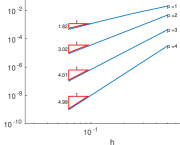
(b) 3D steady transport

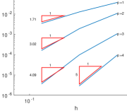
(c) shallow water equation

Fig. 1: h-convergence of the HDG method using the eHDG solver.

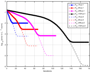
(a) Error history for p=1,2

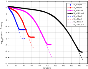
(b) Error history for p=3,4

Fig. 2: Convergence of eHDG for different $h$ and $p$ for 2D transport smooth solution.

Table 1: Iterations for 2D transport equation with smooth and discontinuous solutions and 3D steady state transport equation

$N_{el}(2D)$	$N_{el}(3D)$	p	2D smooth	2D discontinuous	3D steady
16	8	1	45	59	33
64	64	1	67	84	51
256	512	1	107	129	79
1024	4096	1	177	209	130
16	8	2	47	61	39
64	64	2	67	87	51
256	512	2	101	133	76
1024	4096	2	179	214	131
16	8	3	46	65	39
64	64	3	66	92	49
256	512	3	108	135	79
1024	4096	3	186	211	136
16	8	4	45	66	35
64	64	4	68	90	51
256	512	4	112	128	83
1024	4096	4	189	198	143

Figure 1 shows the $h$-convergence of the HDG discretization with eHDG iterative solver. The convergence is optimal i.e. $(p+1)$ for a polynomial order $p$. The tolerance criteria for the eHDG solver is set as follows:

$$|\|u^{k}-u_{e}\|_{{L^{2}\left(\Omega\right)}}-\|u^{k-1}-u_{e}\|_{{L^{2}\left(\Omega\right)}}|<10^{-10}.$$ (10)

Thus the succesive difference in $L^{2}$ norm of error between numerical solution and exact solution is used as a criteria for tolerance in this case.

Figure 2 shows the convergence history of the eHDG solver in the log-linear scale. As proved in Theorem 1 the eHDG is exponential convergent in the iteration $k$. Also the stagnation region observed near the end of each curve is due to the fact that for a particular mesh size $h$ and polynomial order $p$ we can achieve only as much accuracy as prescribed by the HDG discretization error and cannot go beyond that. The numerical results for different solution orders also verify the fact that the convergence of eHDG method is independent of the polynomial order $p$. This can also be seen from the $4$th column of Table 1.

4.2 2D steady state transport equation with discontinuous solution

In this case we take $f=0$ and $\boldsymbol{\beta}=(1+sin(\pi y/2),2)$. The domain $\Omega$ is $[0,2]\times[0,2]$ and the inflow boundary condition is given as

$$g=\left\{\begin{array}[]{ll}1&x=0,0\leq y\leq 2\\ \sin^{6}\left(\pi x\right)&0<x\leq 1,y=0\\ 0&1\leq x\leq 2,y=0\end{array}\right..$$

We choose a slight different stopping criteria to avoid the exact solution:

$$\|u^{k}-u^{k-1}\|_{{L^{2}\left(\Omega\right)}}<10^{-10}.$$

The evolution of solution with iterations obtained for $32\times 32$ elements and polynomial order $4$ is shown in Figure 3. As shown from the $5$th column of Table 1, due to the discontinuity, the eHDG solver takes a slightly more iterations compared to the smooth solution case, but the number of iteration is still (almost) independent of the solution order. Also we observe that the solution evolves from inflow to outflow. This can be proved rigorously, but for the space limitation, the proof is omitted.

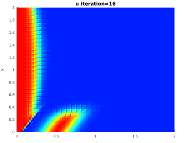
(a) $u$ at $iteration=16$

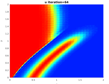
(b) $u$ at $iteration=64$

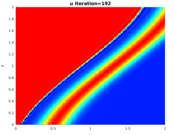
(c) $u$ at $iteration=192$

Fig. 3: Evolution of solution with respect to iterations for upwind HDG

4.3 3D steady state transport equation

In this example we choose $\boldsymbol{\beta}=(z,x,y)$ in (1) and the following exact solution:

$$u^{e}=\frac{1}{\pi}\sin(\pi x)\cos(\pi y)\sin(\pi z).$$

The forcing is selected in such a way that it corresponds to the exact solution selected. Here, the domain is $[0,1]\times[0,1]\times[0,1]$ with $x=0$, $y=0$ and $z=0$ as inflow boundaries. A structured $16\times 16\times 16$ hexahedral mesh is used for all simulations. The tolerance critera used is same as in section 4.1. Similar to the 2D example in section 4.1, we obtain the optimal convergence rates as shown in Figure 1(b).

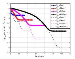
(a) Error history for p=1,2

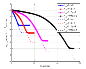
(b) Error history for p=3,4

Fig. 4: Convergence of eHDG for different $h$ and $p$ for 3D transport.

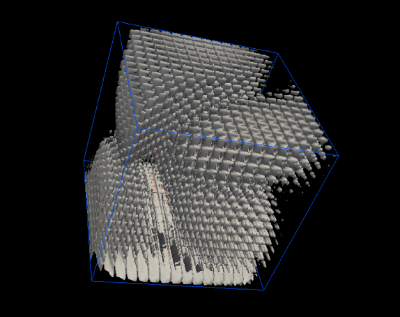
(a) $u$ at $iteration=1$

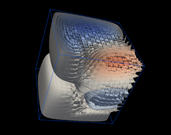
(b) $u$ at $iteration=16$

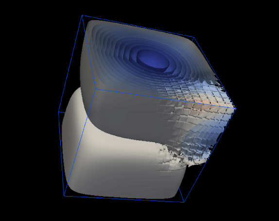
(c) $u$ at $iteration=48$

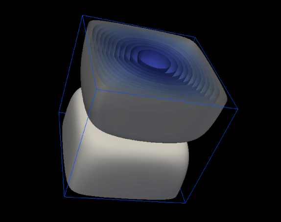
(d) $u$ at $iteration=143$

Fig. 5: Evolution of iterative eHDG solutions for 3D steady state transport equation.

The convergence history is shown in figure 4 and they exhibit a similar trend as in 2D, i.e. exponential convergence independent of the polynomial order (see also the $6$th column of Table 1. Again the iteration increases as the mesh is refined. The evolution of the eHDG solution with respect to iterations in Figure 5 shows the convergence of solution from inflow to outflow. Here, the solution order is $p=4$.

4.4 2D linearized shallow water equations

Here we consider equation (6), and in that we are considering a linear standing wave, which is an oceanic flow. For linear standing wave we take $\Phi=g=1$, $f=0$, $\gamma=0$ (zero bottom friction), ${\boldsymbol{\tau}}=0$ (zero wind stress). The domain is $[0,1]\times[0,1]$ and wall boundary condition is applied on the boundary. The following exact solution [16] is taken

$$\phi =\cos(\pi x)\cos(\pi y)\cos(\sqrt{2}\pi t),$$ (11a)

$$u =\frac{1}{\sqrt{2}}\sin(\pi x)\cos(\pi y)\sin(\sqrt{2}\pi t),$$ (11b)

$$v =\frac{1}{\sqrt{2}}\cos(\pi x)\sin(\pi y)\sin(\sqrt{2}\pi t).$$ (11c)

The convergence of the $L^{2}$ norm of the solution is presented in Figure 1. Here we have taken $\Delta t=10^{-6}$ and $10^{5}$ time steps in order to show the theoretical convergence rates and from Figure 1(c) we see that optimal convergence rate is obtained. The number of iterations required per time step in this case is constant and is always equal to $2$ for all meshes and polynomial orders considered. The reason is that the initial guess for each time step is taken as the solution in the previous time step. Furthermore, the time step is small.

Table 2: Iterations per time step for 2D linearized shallow water equation and 3D time dependent advection for different $\Delta t$

$N_{el}(2D)$	$N_{el}(3D)$	p	2D Shallow water		3D advection
			$\Delta t=10^{-3}$	$\Delta t=10^{-4}$	$\Delta t=10^{-3}$	$\Delta t=10^{-4}$
16	8	1	3	2	2	2
64	64	1	4	2	3	2
256	512	1	4	3	3	2
1024	4096	1	4	3	3	2
16	8	2	4	2	2	2
64	64	2	4	2	3	2
256	512	2	5	2	3	2
1024	4096	2	6	3	3	2
16	8	3	4	2	3	2
64	64	3	4	2	3	2
256	512	3	5	3	3	2
1024	4096	3	6	3	4	2
16	8	4	4	2	3	2
64	64	4	5	3	3	2
256	512	4	6	3	3	2
1024	4096	4	7	3	4	2

To compare with the 3D time-dependent advection in the next section, we choose the time step of $\Delta t=10^{-3}$ and $\Delta t=10^{-4}$, and tabulate the number of eHDG iterations in Table 2. As can be seen, the number of iterations increases slightly as we increase the solution order, and this is consistent with Theorem 2.

4.5 3D time dependent transport equation

In this section we consider the following time-dependent transport equation

$$\frac{\partial u}{\partial t}+\nabla\cdot(\boldsymbol{\beta}u)=f,$$ (12)

and the exact solution is a Gaussian moving across the diagonal of a unit cube, i.e.,

$$u^{e}=e^{-5((x-0.2t)^{2}+(y-0.2t)^{2}+(z-0.2t)^{2})},$$

Structured hexahedral mesh $8\times 8\times 8$ is used and the solution order is $p=4$. The time step is chosen $\Delta t=0.01$ and the simulation is run for $240$ time steps. Figure 6 compares the numerical solution using the eHDG iterative solver and the exact solution. The tolerance criteria the same as in Section 4.1, and the solver always takes 9 iterations per time step. In table 2 we compare the iterations per time step required to converge for two smaller time step sizes. Unlike shallow water equation, transport equation with eHDG iterative solver has constant eHDG iterations as the solution increases, and this is consistent with our theoretical result in Theorem 5.

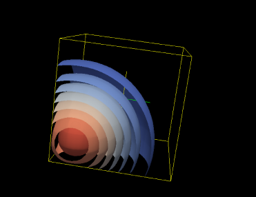
(a) $u$ at $time=0.5$

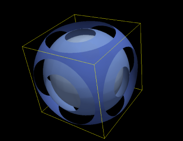
(b) $u$ at $time=1.4$

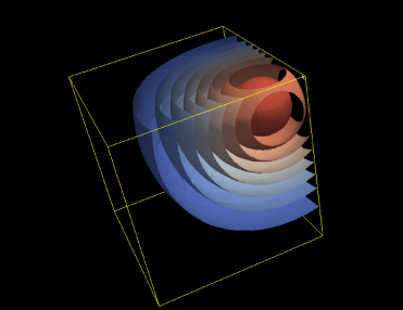
(c) $u$ at $time=2.4$

Fig. 6: eHDG solution for 3D time dependent transport equation

5 Conclusion

We have presented an iterative solver, namely eHDG, for HDG discretizations of hyperbolic systems. The method exploits the structure of HDG discretization and idea from domain decomposition methods. The key features of the eHDG solver are: 1) it solves independent element-by-element local equations during each iteration, 2) the number of iterations are independent of polynomial order, and 3) it achieves exponential convergence rate. These features make the eHDG solver naturally suitable for higher order HDG methods in large scale parallel environments.

References

- [1] D. Bennequin, M. J. Gander, and L. Halpern, A homographic best approximation problem with application to optimized Schwarz waveform relaxation, Math. Comp., 78 (2009), pp. 185–223.
- [2] A. Breuer, A. Heinecke, S. Rettenberger, M. Bader A.A. Gabriel, and C. Pelties, Supercomputing, Springer, 2013, ch. Sustained Petascale Performance of Seismic Simulations With SeisSol on SuperMUC, pp. 1–18.
- [3] T. Bui-Thanh, From Godunov to a unified hybridized discontinuous Galerkin framework for partial differential equations, Journal of Computational Physics, 295 (2015), pp. 114–146.
- [4] , From Rankine-Hugoniot Condition to a Constructive Derivation of HDG Methods, Lecture Notes in Computational Sciences and Engineering, Springer, 2015, pp. 483–491.
- [5] Tan Bui-Thanh, Hybridized discontinuous Galerkin methods for linearized shallow water equations, Submitted, (2015).
- [6] Tan Bui-Thanh, Carsten Burstedde, Omar Ghattas, James Martin, Georg Stadler, and Lucas C. Wilcox, Extreme-scale UQ for Bayesian inverse problems governed by PDEs, in SC12: Proceedings of the International Conference for High Performance Computing, Networking, Storage and Analysis, 2012. Gordon Bell Prize finalist.
- [7] B. Cockburn, B. Dong, J. Guzman, M. Restelli, and R. Sacco, A hybridizable discontinuous Galerkin method for steady state convection-diffusion-reaction problems, SIAM J. Sci. Comput., 31 (2009), pp. 3827–3846.
- [8] B. Cockburn and J. Gopalakrishnan, The derivation of hybridizable discontinuous Galerkin methods for Stokes flow, SIAM J. Numer. Anal, 47 (2009), pp. 1092–1125.
- [9] Bernardo Cockburn, Jay Gopalakrishnan, and Raytcho Lazarov, Unified hybridization of discontinuous Galerkin, mixed, and continuous Galerkin methods for second order elliptic problems, SIAM J. Numer. Anal., 47 (2009), pp. 1319–1365.
- [10] Bernardo Cockburn, Jay Gopalakrishnan, and Francisco-Javier Sayas, A projection-based error analysis of HDG methods, Mathematics Of Computation, 79 (2010), pp. 1351–1367.
- [11] Bernardo Cockburn, George E. Karniadakis, and Chi-Wang Shu, Discontinuous Galerkin Methods: Theory, Computation and Applications, Lecture Notes in Computational Science and Engineering, Vol. 11, Springer Verlag, Berlin, Heidelberg, New York, 2000.
- [12] J. Cui and W. Zhang, An analysis of HDG methods for the Helmholtz equation, IMA J. Numer. Anal., 34 (2014), pp. 279–295.
- [13] H. Egger and J. Schoberl, A hybrid mixed discontinuous Galerkin finite element method for convection-diffusion problems, IMA Journal of Numerical Analysis, 30 (2010), pp. 1206–1234.
- [14] Martin J. Gander, Loïc Gouarin, and Laurence Halpern, Optimized Schwarz waveform relaxation methods: a large scale numerical study, in Domain decomposition methods in science and engineering XIX, vol. 78 of Lect. Notes Comput. Sci. Eng., Springer, Heidelberg, 2011, pp. 261–268.
- [15] Martin J. Gander and Soheil Hajian, Analysis of Schwarz methods for a hybridizable discontinuous Galerkin discretization, SIAM J. Numer. Anal., 53 (2015), pp. 573–597.
- [16] F. X. Giraldo and T. Warburton, A high-order triangular discontinous Galerkin oceanic shallow water model, International Journal For Numerical Methods In Fluids, 56 (2008), pp. 899–925.
- [17] R. Griesmaier and P. Monk, Error analysis for a hybridizable discontinous Galerkin method for the Helmholtz equation, J. Sci. Comput., 49 (2011), pp. 291–310.
- [18] Laurence Halpern, Optimized Schwarz waveform relaxation: roots, blossoms and fruits, in Domain decomposition methods in science and engineering XVIII, vol. 70 of Lect. Notes Comput. Sci. Eng., Springer, Berlin, 2009, pp. 225–232.
- [19] Laurence Halpern and Jérémie Szeftel, Nonlinear nonoverlapping Schwarz waveform relaxation for semilinear wave propgation, Math. Comp., 78 (2009), pp. 865–889.
- [20] C. Johnson and J. Pitkäranta, An analysis of the discontinuous Galerkin method for a scalar hyperbolic equation, Mathematics of Computation, 46 (1986), pp. 1–26.
- [21] R. M. Kirby, S. J. Sherwin, and B. Cockburn, To CG or to HDG: A comparative study, J. Sci. Comput., 51 (2012), pp. 183–212.
- [22] P. LeSaint and P. A. Raviart, On a finite element method for solving the neutron transport equation, in Mathematical Aspects of Finite Element Methods in Partial Differential Equations, C. de Boor, ed., Academic Press, 1974, pp. 89–145.
- [23] L. Li, S. Lanteri, and R. Perrrussel, A hybridizable discontinuous Galerkin method for solving 3D time harmonic Maxwell’s equations, in Numerical Mathematics and Advanced Applications 2011, Springer, 2013, pp. 119–128.
- [24] P.-L. Lions, On the Schwarz alternating method. I, in First International Symposium on Domain Decomposition Methods for Partial Differential Equations (Paris, 1987), SIAM, Philadelphia, PA, 1988, pp. 1–42.
- [25] , On the Schwarz alternating method. II. Stochastic interpretation and order properties, in Domain decomposition methods (Los Angeles, CA, 1988), SIAM, Philadelphia, PA, 1989, pp. 47–70.
- [26] , On the Schwarz alternating method. III. A variant for nonoverlapping subdomains, in Third International Symposium on Domain Decomposition Methods for Partial Differential Equations (Houston, TX, 1989), SIAM, Philadelphia, PA, 1990, pp. 202–223.
- [27] D. Moro, N. C. Nguyen, and J. Peraire, Navier-Stokes solution using hybridizable discontinuous Galerkin methods, American Institute of Aeronautics and Astronautics, 2011-3407 (2011).
- [28] N. C. Nguyen, J. Peraire, and B. Cockburn, An implicit high-order hybridizable discontinuous Galerkin method for linear convection-diffusion equations, Journal Computational Physics, 228 (2009), pp. 3232–3254.
- [29] , A hybridizable discontinous Galerkin method for Stokes flow, Comput Method Appl. Mech. Eng., 199 (2010), pp. 582–597.
- [30] , High-order implicit hybridizable discontinuous Galerkin method for acoustics and elastodynamics, Journal Computational Physics, 230 (2011), pp. 3695–3718.
- [31] , Hybridizable discontinuous Galerkin method for the time harmonic Maxwell’s equations, Journal Computational Physics, 230 (2011), pp. 7151–7175.
- [32] , An implicit high-order hybridizable discontinuous Galerkin method for the incompressible Navier-Stokes equations, Journal Computational Physics, 230 (2011), pp. 1147–1170.
- [33] W. H. Reed and T. R. Hill, Triangular mesh methods for the neutron transport equation, Tech. Report LA-UR-73-479, Los Alamos Scientific Laboratory, 1973.
- [34] Minh-Binh Tran, Parallel Schwarz waveform relaxation method for a semilinear heat equation in a cylindrical domain, C. R. Math. Acad. Sci. Paris, 348 (2010), pp. 795–799.
- [35] Lucas C. Wilcox, Georg Stadler, Carsten Burstedde, and Omar Ghattas, A high-order discontinuous Galerkin method for wave propagation through coupled elastic-acoustic media, Journal of Computational Physics, 229 (2010), pp. 9373–9396.