The Inclusion of Two-Loop SUSYQCD Corrections to Gluino and Squark Pole Masses in the Minimal and Next-to-Minimal Supersymmetric Standard Model: SOFTSUSY3.7

Abstract

We describe an extension of the SOFTSUSY spectrum calculator to include two-loop supersymmetric QCD (SUSYQCD) corrections of order $\mathcal{O}(\alpha_{s}^{2})$ to gluino and squark pole masses, either in the minimal supersymmetric standard model (MSSM) or the next-to-minimal supersymmetric standard model (NMSSM). This document provides an overview of the program and acts as a manual for the new version of SOFTSUSY, which includes the increase in accuracy in squark and gluino pole mass predictions.

1 Program Summary

Program title: SOFTSUSY
Program obtainable from: http://softsusy.hepforge.org/
Distribution format: tar.gz
Programming language: C++, fortran, C
Computer: Personal computer.
Operating system: Tested on Linux 3.4.6, Mac OS X 10.7.5
Word size: 64 bits.
External routines: None
Typical running time: 15 seconds per parameter point.
Nature of problem: Calculating supersymmetric particle spectrum, mixing parameters and couplings in the MSSM or the NMSSM. The solution to the renormalisation group equations must be consistent with theoretical boundary conditions on supersymmetry breaking parameters, as well as a weak-scale boundary condition on gauge couplings, Yukawa couplings and the Higgs potential parameters.
Solution method: Nested fixed point iteration.
Restrictions: SOFTSUSY will provide a solution only in the perturbative regime and it assumes that all couplings of the model are real (i.e. $CP-$conserving). If the parameter point under investigation is non-physical for some reason (for example because the electroweak potential does not have an acceptable minimum), SOFTSUSY returns an error message. The higher order corrections included are for the MSSM ($R-$parity conserving or violating) or the real $R-$parity conserving NMSSM only.
CPC Classification: 11.1 and 11.6.
Does the new version supersede the previous version?: Yes.
Reasons for the new version: It is desirable to improve the accuracy of the squark and gluinos mass predictions, since they strongly affect supersymmetric particle production cross-sections at colliders.
Summary of revisions: The calculation of the squark and gluino pole masses is extended to be of next-to-next-to leading order in SUSYQCD, i.e. including terms up to ${\mathcal{O}}(g_{s}^{4}/(16\pi^{2})^{2})$.

2 Introduction

Near the beginning of LHC Run II at 13 TeV centre of mass collision energy, hopes are high for the discovery of new physics. A much-studied and long-awaited framework for new physics, namely weak-scale superymmetry, is being searched for in many different channels. In the several prominent explicit models of supersymmetry breaking meditaion, the best chance of observing the production and subsequent decay of supersymmetric particles is via squark and/or gluino production. Squarks and gluinos tend to have the largest production cross-sections among the sparticles and Higgs bosons of the MSSM, because they may be produced by tree-level strong interactions, as opposed to smaller electroweak cross sections relevant for the other superparticles. In $R-$parity conserving supersymmetry (popular because of its apparently viable dark matter candidate), squark and/or gluino production may result in a signal of an excess of highly energetic jets in conjunction with large missing transverse momentum with respect to Standard Model predictions. This classic LHC signature was searched for at LHC Run I at 7 and 8 TeV centre of mass energy, but no significant excess above Standard Model backgrounds was observed. Jets plus missing transverse momentum channels then provided the strongest constraints in the constrained minimal supersymmetric standard model, for instance (CMSSM), along with many other models of supersymmetry breaking mediation.

The higher collision energy at Run II allows for new MSSM parameter space to be explored. In the event of a discovery of the production of supersymmetric particles, one will want to first interpret their signals correctly, and then make inferences about the superymmetry breaking parameters. In order to do this with a greater accuracy, we must use higher orders in perturbation theory. Of particular interest is the connection between the supersymmetric masses of the squarks and gluinos and the experimental observables (functions of jet and missing momenta). The experimental observables may be used to infer pole (or kinematic) masses of the supersymmetric particles, which may then be connected via perturbation theory to the more fundamental supersymmetry breaking parameters in the Lagrangian. These could then be used to test the underlying supersymmetry breaking mediation mechanism [1, 2]. Conversely, if no significant signal for supersymmetry is to be found at the LHC, we shall want to interpret the excluded parameter space in terms of the fundamental supersymmetry breaking parameters. Again, this connection is sensitive (for identical reasons to the discovery case) to the order in perturbation theory which is used. In the most easily accessible channels at the LHC (squark/gluino production), it is useful therefore to use higher orders in the QCD gauge coupling, since this is the largest relevant expansion parameter.

State-of-the art publicly available NMSSM or MSSM spectrum generators such as ISAJET [3], FlexibleSUSY [4], NMSPEC [5], SUSPECT [6], SARAH [7], SPHENO [8], SUSEFLAV [9] or previous versions of SOFTSUSY [10], do not have the complete ${\mathcal{O}}(\alpha_{s}^{2}/(16\pi^{2}))$ two-loop corrections to gluino and squark masses included, despite their being calculated and presented in the literature [11, 12, 13]. Here, we describe their inclusion into the MSSM spectrum calculation in the popular SOFTSUSY program, making them publicly available for the first time. As we emphasised above, we expect them to be useful in increasing the accuracy of inference from data of supersymmetry breaking in the squark and gluino sectors.

The paper proceeds as follows: in the next section, the higher order terms that are included are briefly reviewed. We then provide an example of their effect on a line through CMSSM space. After a summary, the appendices contain technical information on how to compile and run SOFTSUSY including the higher order terms.

3 Higher Order Terms

Two-loop contributions to fermion pole masses in gauge theories were calculated in Ref. [11] and these results are specialised to compute the gluino pole mass. Depending upon the ratio $m_{\tilde{q}}/m_{\tilde{g}}$, a two-loop correction of up to several percent was found. On the other hand, Ref. [12] calculated the two-loop contributions to scalar masses from gauge theory and these results are specialised to the two-loop squark masses, where corrections up to about one percent were noted. In both cases, the results were obtained in the $\overline{\rm DR}^{\prime}$ renormalization scheme [14], consistent with the renormalization group equations used in softly broken supersymmetric models. The version of SOFTSUSY described here now contains these computations [11, 12]. A library for computing two-loop self-energy integrals, TSIL [15], is included within the SOFTSUSY distribution; there is no need to download it separately.

In addition, the gluino result has been improved by re-expanding the gluino self-energy function squared mass arguments around the gluino, squark, and top quark pole masses, as described in Ref. [13]. This requires iteration to determine the gluino pole mass, and hence is slower than simply evaluating the self-energy functions with the lagrangian mass parameters, but the accuracy of the calculation is improved significantly [13]. Typically, 4 to 6 iterations are required to reach the default tolerance of less than 1 part in $10^{5}$ difference between successive iterations for the gluino pole mass. This iteration is not the bottleneck in the calculation, as we find that the CPU time spent on the squark masses is about twice that spent on the gluino mass, even with 6 iterations for the latter. We did not implement this improvement for the squarks since the effect is less significant, and the necessary iterations would be much slower.

3.1 Kinky Masses

In implementing these 2-loop pole masses, we encountered an interesting issue that does not seem to have been noted before, as far as we know. Consider the self-energy and pole mass of a particle $Z$ that has a three-point coupling to particles $X$ and $Y$. Let the tree-level squared masses of these particles by $z$, $x$, and $y$ respectively. If $z$ happens to be close to the threshold value $(\sqrt{x}+\sqrt{y})^{2}$, then the computed 2-loop complex pole mass of $Z$ will have a singularity proportional to

$$1/\sqrt{-\delta-i\epsilon}$$ (1)

where $\epsilon$ is infinitesimal and positive, and

$$z=(\sqrt{x}+\sqrt{y})^{2}(1+\delta).$$ (2)

The reason for this can be understood from the sequence of Feynman diagrams shown in Figure 1. After reduction to basis integrals, the result of Figure 1(b) contains terms proportional to $V(x,y,u,v)$ and $B(x,y^{\prime})$, in the notation of refs. [16, 15]. (Here the prime represents a derivative with respect to the corresponding argument, and the external momentum invariant is $s=z$.)

Figure 1: Feynman diagrams for the self-energy of a particle that couples to two lighter particles. The dark blobs in (b) and (c) represent 1-loop subdiagrams. Near threshold, diagrams (b) and (c) have $1/(-\delta)^{1/2}$ and $1/(-\delta)^{3/2}$ singularities, respectively, where $s=(\sqrt{x}+\sqrt{y})^{2}(1+\delta)$, with $x$ and $y$ the squared masses of the internal particles.

Then, for example, one can evaluate:

$$B(x,y^{\prime})\Big{|}_{s=(\sqrt{x}+\sqrt{y})^{2}(1+\delta)} = -\frac{\pi(x/y)^{1/4}}{(\sqrt{x}+\sqrt{y})^{2}\sqrt{-\delta-i\epsilon}}+\ldots~{}.$$ (3)

We have found that in general such singularities do not cancel within the fixed-order 2-loop pole mass calculation. This includes e.g. the pole mass of the gluino, where we checked that there are singularities in the pole mass as one varies the top mass and one of the stop masses very close to the 2-body decay threshold. Similarly, there are singularities in the 2-loop pole masses of the top squarks, in each case when the top mass and the gluino happen to be very close to the 2-body decay thresholds. We have also checked that this behavior occurs in a simple toy model involving only three massive scalar particles.

This singular behavior might be quite surprising, because the pole mass is supposed to be an observable, and therefore ought to be free of divergences of any kind. The resolution is that, similar to problems with infrared divergences, the singularity is an artifact of truncating perturbation theory. The 3-loop diagram of Figure 1(c) will diverge like $1/(-\delta)^{3/2}$, and similar diagrams of loop order $L$ will diverge like $1/(-\delta)^{L-3/2}$. These contributions can presumably be resummed to give a result that is well-behaved as $\delta\rightarrow 0$, although proving that is beyond the scope of the present paper.

The above singularity behavior is not tied to the presence of massless gauge bosons. However, if massless gauge bosons are present, then there is another, less severe, type of singular threshold behavior, due to the Feynman diagram shown in Figure 2.

Figure 2: Feynman diagram for the self-energy of a particle that couples to two lighter particles, each of which couples to a massless gauge boson. Near threshold, this diagram has a $\ln(-\delta)$ singularity, where $s=(\sqrt{x}+\sqrt{y})^{2}(1+\delta)$, with $x$ and $y$ the squared masses of the internal particles.

In the notation of refs. [16, 15], this arises due to the near-threshold dependence of the corresponding self-energy basis integral:

$$M(x,x,y,y,0)\Big{|}_{s=(\sqrt{x}+\sqrt{y})^{2}(1+\delta)} = -\frac{2\pi^{2}}{(\sqrt{x}+\sqrt{y})^{2}}\ln(-\delta-i\epsilon)+\ldots~{}.$$ (4)

Again, the singularity in the computed 2-loop pole mass is an artifact of the truncation of perturbation theory, and would presumably be removed by a resummation including all diagrams with $2,3,4,\ldots$ massless gauge bosons exchanged between particles $X$ and $Y$.

Note that it requires some bad luck to encounter any of these threshold singularity problems in practice, as there is no good reason why the tree-level masses should be tuned to the high precision necessary to make the problem numerically significant. Nevertheless, it could lead to a small “kink” in the computed pole mass if one performs a scan over models by varying the input masses. To avoid this possibility, in our code we test for small $\delta$, and then replace the offending 2-loop self-energy basis integrals $B(x,y^{\prime})$ and $V(x,y,u,v)$ and $M(x,x,y,y,0)$ by values interpolated from slightly larger and smaller values of the external momentum invariant. Explicitly, if $\delta<t$ (we choose $t=0.04$ in the current version of SOFTSUSY, with the value controlled by the quantity THRESH_TOL in src/supermodel/supermodel/sumo_params.h), the integral in question $I(s)$ is replaced by

$$I(s)\approx\frac{1}{2}\left(1+\frac{\delta}{t}\right)I\left([1+t]s\right)+\frac{1}{2}\left(1-\frac{\delta}{t}\right)I\left([1-t]s\right).$$ (5)

This provides a pole mass that varies continuously in scans of input masses near thresholds, and the difference between our value and the value that would be obtained by a proper resummation should be small.

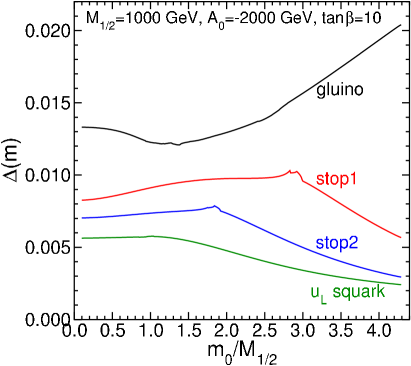
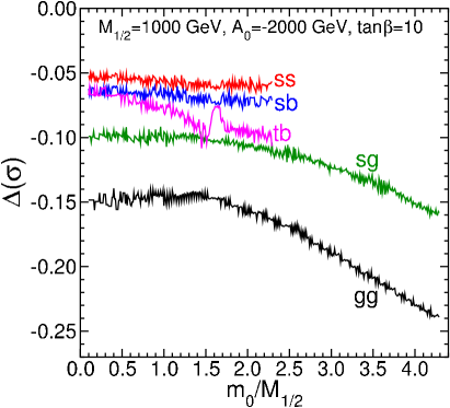
Figure 3: Effects of the 2-loop SUSYQCD corrections to sparticle pole masses (left panel) and total production cross-sections (right panel), for a line in CMSSM space with $M_{1/2}=1$ TeV, $A_{0}=-2$ TeV, $\tan\beta=10$ and $\mu>0$. In the left panel, $\Delta(m)=m_{\textrm{2-loop}}/m_{\textrm{1-loop}}-1$, where $m_{\textrm{2-loop}}$ is the pole mass calculated including the ${\mathcal{O}}(\alpha_{s}^{2}/(16\pi^{2}))$ terms whereas $m_{\textrm{1-loop}}$ is the pole mass calculated at one-loop order. In the right panel, $\Delta(\sigma)=\sigma_{\textrm{2-loop}}/\sigma_{\textrm{1-loop}}-1$, where $\sigma_{\textrm{2-loop}}$ is the 13 TeV LHC production cross-section calculated using the ${\mathcal{O}}(\alpha_{s}^{2}/(16\pi^{2}))$ terms in pole masses whereas $\sigma^{\textrm{1 loop}}$ is the 13 TeV LHC production cross-section calculated with one-loop pole masses. The label ‘gg’ refers to gluino-gluino production, ‘sg’ to squark-gluino plus antisquark-gluino, ‘ss’ to squark-squark plus antisquark-antisquark, ‘sb’ to squark-antisquark, and ‘tb’ to stop-antistop production. The cross-sections in each case are obtained at NLL+NLO using NLL-fastv3.1-13TeV [17, 18, 19, 20, 18, 21, 22, 23, 24]. .

3.2 Illustration of Results

We now illustrate the effect of the ${\mathcal{O}}(\alpha_{s}^{2}/(16\pi^{2}))$ corrections to gluino and squark pole masses, taking the constrained minimal supersymmetric standard model (CMSSM) pattern of MSSM supersymmetry breaking Lagrangian terms. In the CMSSM, at the gauge unification scale $\sim{\mathcal{O}}(10^{16})\textrm{~{}GeV}$ the gaugino masses are set equal to $M_{1/2}$, the scalar masses are set to a universal flavour diagonal mass $m_{0}$ and the soft supersymmetry breaking trilinear scalar couplings are set equal to a massive parameter $A_{0}$ times the relevant Yukawa coupling. Here, for illustration, we set $M_{1/2}=1$ TeV, $A_{0}=-2\>{\rm TeV}$, the ratio of the MSSM’s two Higgs vacuum expectation values $\tan\beta=10$ and the sign of the Higgs superpotential parameter term $\mu$ to be positive. We then allow $m_{0}$ to vary, and plot the relative difference caused by the new higher order terms in Fig. 3a. For this illustration, we have not included two-loop corrections to gauge and Yukawa couplings and three-loop renormalisation group equations for the superpotential parameters [25], although with them, the results are qualitatively similar. The overall message from the figure is that differences of percent level order in the pole masses of gluinos and squarks arise from the higher order corrections. In Fig. 3a, the plot does not extend to larger values of $m_{0}/M_{1/2}$, because there is no phenomenologically acceptable electroweak symmetry breaking there (the superpotential $\mu$ term becomes imaginary at the minimum of the potential, indicating a saddle point). The rough size of the two-loop correction is consistent with that estimated in the previous literature [11, 12, 13]. Note that there are wiggles in the $\tilde{g}$, $\tilde{t}_{1}$, and $\tilde{t}_{2}$ curves, near $m_{0}/M_{1/2}=1.35$, $2.9$, and $1.9$, respectively. These are the remnants of the instabilities mentioned in section 3.1 after smoothing by the interpolation procedure described there, with $t=0.04$. These correspond to the thresholds for the decays $\tilde{g}\rightarrow t\tilde{t}_{1}$ and $\tilde{t}_{1}\rightarrow t\tilde{g}$ and $\tilde{t}_{2}\rightarrow t\tilde{g}$, respectively. Although the remaining wiggles are visible on the plot, they are small in absolute terms, and are of order the uncertainties due to higher-order corrections.

In Fig. 3b, we show the concomitant effect on the various next-to-leading order sparticle production cross-sections at the 13 TeV LHC by using NLL-Fast3.1 [17, 18, 19, 20, 18, 21, 22, 23, 24]. NLL-Fast3.1 calculates at the next-to-leading order (NLO) in supersymmetric QCD, with next-to-leading logarithm (NLL) re-summation. However, it is based on fixed interpolation tables with only 3 significant digits, resulting in a visible jaggedness of the points in the figure. Nonetheless, we see that the change in the gluino mass due to next-to-next-to leading order (NNLO) effects leads to a large 15-25$\%$ reduction in the production cross-section. Other sparticle production cross-section modes shown decrease by more than 5$\%$, thus accounting for these NNLO effects is important in reducing the theoretical uncertainties. Some of the curves terminate when $m_{0}/M_{1/2}>2.3$ because NLL-Fast3.1 considers the production cross-sections to be too small to be relevant, and so returns zeroes.

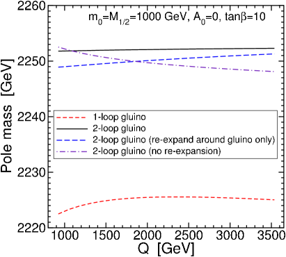
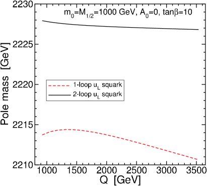
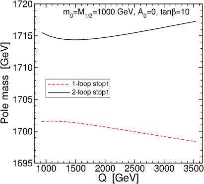
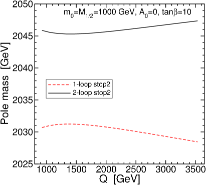
Figure 4: Scale dependences of gluino and squark pole mass predictions for the CMSSM with $m_{0}=M_{1/2}=1$ TeV, $A_{0}=0$, $\tan\beta=10$ and $\mu>0$, comparing 1-loop and 2-loop approximations. The upper left panel is for the gluino, upper right panel for $\tilde{u}_{L}$, lower left panel for $\tilde{t}_{1}$, and lower right panel for $\tilde{t}_{2}$. In the case of the gluino, the solid line uses the re-expansion of squared mass arguments about the gluino and squark pole masses as described in [13]; this is the default used by SOFTSUSY for the gluino when the higher-order pole mass calculations are enabled.

In Fig. 4, we illustrate the renormalization scale $(Q)$ dependences of the computed gluino and squark pole masses, by varying the scale $Q$ at which the masses are calculated by a factor of 2 around $M_{SUSY}=\sqrt{m_{{\tilde{t}}_{1}}m_{{\tilde{t}}_{2}}}$. We see the expected reduced scale dependence going from 1-loop to 2-loop order. In the case of the gluino, we also see that the 2-loop calculation using a re-expansion around both the squark and gluino pole masses, as described in [13], displays less renormalization scale dependence than the case where only the gluino mass is re-expanded around its pole mass in the gluino pole mass calculation, or the case in which no re-expansion is used. This is consistent with the suggestion in [13] that the perturbation expansion is made more convergent by re-expanding around pole masses rather than around the running masses. For this reason, the re-expansion method is used as the default by SOFTSUSY when the higher-order pole masses are enabled. In the cases of the squark masses, the improvement of the renormalization scale dependence of the computed pole mass is less significant going from 1-loop to 2-loop order. We also note that in each case, the 2-loop correction is much larger than the scale dependence in the 1-loop result. Thus, as usual, the renormalization scale dependence gives only a lower bound, and not a reliable estimate, of the remaining theoretical error.

4 Summary and Conclusions

Two-loop ${\mathcal{O}}(\alpha_{s}^{2}/(16\pi^{2}))$ are now included in the public release of SOFTSUSY, and so are available for use. We have demonstrated that along a typical line in CMSSM space, they are responsible for around $\mathcal{O}(1\%)$ relative changes in the squark and gluino masses, which will change their various production cross-sections by around $5-25\%$. The largest 2-loop SUSYQCD pole mass correction is for the gluino, and it increases as the squarks become heavier than the gluino, reaching 2% when $m_{0}/M_{1/2}=4$. These sources of theoretical error can now be taken into account and consequently reduced by using the new version of SOFTSUSY. In turn, the connection between measurements and various Lagrangian parameters (in particular, soft supersymmetry breaking sparticle mass parameters) is made more accurate. Thus, fits of the MSSM or NMSSM to cosmological and collider data will have a smaller associated theoretical error (as would studies of the unification of sparticle masses were there to be a discovery and subsequent measurement of sparticles). Other increases in MSSM or NMSSM mass prediction accuracy await future work: Higgs mass predictions, gauginos and sleptons, for instance.

Appendix A Installation of the Increased Accuracy Mode

In order to have SOFTSUSY use the higher order corrections described in the present paper, the code containing them must be both compiled and a run-time flag should be set to ensure their employment in the spectrum calculation. A compilation argument to the ./configure command is provided in order to compile the necessary code to include the higher order corrections:

--enable-two-loop-sparticle-mass-compilation

We have included a global boolean variable which controls the higher order corrections at run time (provided that the program has already been compiled with the higher order corrections included):

bool USE_TWO_LOOP_SPARTICLE_MASS - if true, the $\mathcal{O}(\alpha_{s}^{2})$ corrections are included (corresponds to the SOFTSUSY Block parameter 22 in the SOFTSUSY block of the SUSY Les Houches Accord input).

By default, the higher order corrections are switched off (the boolean value is set to false), unless the user sets it in their main program, or in the input parameters (see B). One can choose to include the two-loop $\mathcal{O}(\alpha_{s}^{2})$ corrections to gluino and squark pole masses independently of whether one includes two-loop corrections to the extracted MSSM value of $\alpha_{s}(M_{Z})$ or three-loop MSSM renormalisation group equations, as described in Ref. [25].

To summarise, installation is completed by executing the following commands

> ./configure --enable-two-loop-sparticle-mass-compilation
> make

We remind the reader that the two-loop corrections discussed here are available for use either in the MSSM (with or without $R-$parity violation) [26] or in the NMSSM [27].

Appendix B Running SOFTSUSY in the Increased Accuracy Mode

SOFTSUSY produces an executable called softpoint.x. One can run this executable from command line arguments, but the higher order corrections will be, by default, switched off. One may switch the two-loop $\mathcal{O}(\alpha_{s}^{2})$ corrections described in the present paper on with the argument --two-loop-sparticle-masses.

For example:

./softpoint.x sugra --tol=1.0e-5 --m0=250 --m12=100 --a0=-100 --tanBeta=10 --sgnMu=1 \
--two-loop-sparticle-masses --two-loop-sparticle-mass-method=<expandAroundGluinoPole>

The variable expandAroundGluinoPole re-expands the two-loop computation of the gluino mass around the gluino and squark masses if it is set to 3 (default), around only the gluino mass if set to 2 and performs no expansion (but still includes the 2-loop corrections) if it is set to 1.

For the calculation of the spectrum of single points in parameter space, one could alternatively use the SUSY Les Houches Accord (SLHA) [28, 29] input/output option. The user must provide a file (e.g. the example file included in the SOFTSUSY distribution inOutFiles/lesHouchesInput) which specifies the model dependent input parameters. The program may then be run with

 ./softpoint.x leshouches < inOutFiles/lesHouchesInput

One can change whether the higher order corrections are switched on (provided they have been compiled by setting the correct ./configure flag as described above) with SOFTSUSY Block parameter 22 and the two-loop gluino expansion approximation with parameter 23:

Block SOFTSUSY               # Optional SOFTSUSY-specific parameters
   22   1.000000000e+00      # Include 2-loop terms in gluino/squark masses
                             # (default of 0 to disable)
   23   3.000000000e+00      # sets expandAroundGluinoPole parameter (default 3)

Parameter 23 is equal to the integer global variable expandAroundGluinoPole.

We are also providing an example user program called higher.cpp, found in the src/ directory of the SOFTSUSY distribution. Running make in the main SOFTSUSY directory produces an executable called higher.x, which runs without arguments or flags. This program illustrates the implementation of the 2-loop SUSYQCD pole masses, and in particular outputs all of the data used in Figures 3 and 4 above. The file higher.cpp and the output of higher.x (called twoLoop.dat) are also found as ancillary electronic files with the arXiv submission for this article.

References

- [1] B. C. Allanach, G. A. Blair, S. Kraml, H. U. Martyn, G. Polesello, W. Porod, P. M. Zerwas, Reconstructing supersymmetric theories by coherent LHC / LC analysesarXiv:hep-ph/0403133.
- [2] B. C. Allanach, G. A. Blair, A. Freitas, S. Kraml, H. U. Martyn, G. Polesello, W. Porod, P. M. Zerwas, SUSY parameter analysis at TeV and Planck scales, Nucl. Phys. Proc. Suppl. 135 (2004) 107–113, [,107(2004)]. arXiv:hep-ph/0407067, doi:10.1016/j.nuclphysbps.2004.09.052.
- [3] F. E. Paige, S. D. Protopopescu, H. Baer, X. Tata, ISAJET 7.69: A Monte Carlo event generator for pp, anti-p p, and e+e- reactionsarXiv:hep-ph/0312045.
- [4] P. Athron, J.-h. Park, D. Stöckinger, A. Voigt, FlexibleSUSY - A spectrum generator generator for supersymmetric models, Comput. Phys. Commun. 190 (2015) 139–172. arXiv:1406.2319, doi:10.1016/j.cpc.2014.12.020.
- [5] U. Ellwanger, C. Hugonie, NMSPEC: A Fortran code for the sparticle and Higgs masses in the NMSSM with GUT scale boundary conditions, Comput. Phys. Commun. 177 (2007) 399–407. arXiv:hep-ph/0612134, doi:10.1016/j.cpc.2007.05.001.
- [6] A. Djouadi, J.-L. Kneur, G. Moultaka, SuSpect: A Fortran code for the supersymmetric and Higgs particle spectrum in the MSSM, Comput. Phys. Commun. 176 (2007) 426–455. arXiv:hep-ph/0211331, doi:10.1016/j.cpc.2006.11.009.
- [7] F. Staub, SARAHarXiv:0806.0538.
- [8] W. Porod, SPheno, a program for calculating supersymmetric spectra, SUSY particle decays and SUSY particle production at e+ e- colliders, Comput. Phys. Commun. 153 (2003) 275–315. arXiv:hep-ph/0301101, doi:10.1016/S0010-4655(03)00222-4.
- [9] D. Chowdhury, R. Garani, S. K. Vempati, SUSEFLAV: Program for supersymmetric mass spectra with seesaw mechanism and rare lepton flavor violating decays, Comput. Phys. Commun. 184 (2013) 899–918. arXiv:1109.3551, doi:10.1016/j.cpc.2012.10.031.
- [10] B. C. Allanach, SOFTSUSY: a program for calculating supersymmetric spectra, Comput. Phys. Commun. 143 (2002) 305–331. arXiv:hep-ph/0104145, doi:10.1016/S0010-4655(01)00460-X.
- [11] S. P. Martin, Fermion self-energies and pole masses at two-loop order in a general renormalizable theory with massless gauge bosons, Phys. Rev. D72 (2005) 096008. arXiv:hep-ph/0509115, doi:10.1103/PhysRevD.72.096008.
- [12] S. P. Martin, Two-loop scalar self-energies and pole masses in a general renormalizable theory with massless gauge bosons, Phys. Rev. D71 (2005) 116004. arXiv:hep-ph/0502168, doi:10.1103/PhysRevD.71.116004.
- [13] S. P. Martin, Refined gluino and squark pole masses beyond leading order, Phys. Rev. D74 (2006) 075009. arXiv:hep-ph/0608026, doi:10.1103/PhysRevD.74.075009.
- [14] I. Jack, D. R. T. Jones, S. P. Martin, M. T. Vaughn, Y. Yamada, Decoupling of the epsilon scalar mass in softly broken supersymmetry, Phys. Rev. D50 (1994) 5481–5483. arXiv:hep-ph/9407291, doi:10.1103/PhysRevD.50.R5481.
- [15] S. P. Martin, D. G. Robertson, TSIL: A Program for the calculation of two-loop self-energy integrals, Comput. Phys. Commun. 174 (2006) 133–151. arXiv:hep-ph/0501132, doi:10.1016/j.cpc.2005.08.005.
- [16] S. P. Martin, Evaluation of two loop selfenergy basis integrals using differential equations, Phys. Rev. D68 (2003) 075002. arXiv:hep-ph/0307101, doi:10.1103/PhysRevD.68.075002.
- [17] W. Beenakker, C. Borschensky, M. Krämer, A. Kulesza, E. Laenen, S. Marzani, J. Rojo, NLO+NLL squark and gluino production cross-sections with threshold-improved parton distributionsarXiv:1510.00375.
- [18] W. Beenakker, S. Brensing, M. n. Kramer, A. Kulesza, E. Laenen, L. Motyka, I. Niessen, Squark and Gluino Hadroproduction, Int. J. Mod. Phys. A26 (2011) 2637–2664. arXiv:1105.1110, doi:10.1142/S0217751X11053560.
- [19] W. Beenakker, S. Brensing, M. Kramer, A. Kulesza, E. Laenen, I. Niessen, Supersymmetric top and bottom squark production at hadron colliders, JHEP 08 (2010) 098. arXiv:1006.4771, doi:10.1007/JHEP08(2010)098.
- [20] W. Beenakker, M. Kramer, T. Plehn, M. Spira, P. M. Zerwas, Stop production at hadron colliders, Nucl. Phys. B515 (1998) 3–14. arXiv:hep-ph/9710451, doi:10.1016/S0550-3213(98)00014-5.
- [21] W. Beenakker, S. Brensing, M. Kramer, A. Kulesza, E. Laenen, I. Niessen, Soft-gluon resummation for squark and gluino hadroproduction, JHEP 12 (2009) 041. arXiv:0909.4418, doi:10.1088/1126-6708/2009/12/041.
- [22] A. Kulesza, L. Motyka, Soft gluon resummation for the production of gluino-gluino and squark-antisquark pairs at the LHC, Phys. Rev. D80 (2009) 095004. arXiv:0905.4749, doi:10.1103/PhysRevD.80.095004.
- [23] A. Kulesza, L. Motyka, Threshold resummation for squark-antisquark and gluino-pair production at the LHC, Phys. Rev. Lett. 102 (2009) 111802. arXiv:0807.2405, doi:10.1103/PhysRevLett.102.111802.
- [24] W. Beenakker, R. Hopker, M. Spira, P. M. Zerwas, Squark and gluino production at hadron colliders, Nucl. Phys. B492 (1997) 51–103. arXiv:hep-ph/9610490, doi:10.1016/S0550-3213(97)80027-2.
- [25] B. C. Allanach, A. Bednyakov, R. Ruiz de Austri, Higher order corrections and unification in the minimal supersymmetric standard model: SOFTSUSY3.5, Comput. Phys. Commun. 189 (2015) 192–206. arXiv:1407.6130, doi:10.1016/j.cpc.2014.12.006.
- [26] B. C. Allanach, M. A. Bernhardt, Including R-parity violation in the numerical computation of the spectrum of the minimal supersymmetric standard model: SOFTSUSY, Comput. Phys. Commun. 181 (2010) 232–245. arXiv:0903.1805, doi:10.1016/j.cpc.2009.09.015.
- [27] B. C. Allanach, P. Athron, L. C. Tunstall, A. Voigt, A. G. Williams, Next-to-Minimal SOFTSUSY, Comput. Phys. Commun. 185 (2014) 2322–2339. arXiv:1311.7659, doi:10.1016/j.cpc.2014.04.015.
- [28] P. Z. Skands, et al., SUSY Les Houches accord: Interfacing SUSY spectrum calculators, decay packages, and event generators, JHEP 07 (2004) 036. arXiv:hep-ph/0311123, doi:10.1088/1126-6708/2004/07/036.
- [29] B. C. Allanach, et al., SUSY Les Houches Accord 2, Comput. Phys. Commun. 180 (2009) 8–25. arXiv:0801.0045, doi:10.1016/j.cpc.2008.08.004.