Population dynamics method with a multi-canonical feedback control

Abstract

We discuss the Giardinà-Kurchan-Peliti population dynamics method for evaluating large deviations of time averaged quantities in Markov processes [Phys. Rev. Lett. 96, 120603 (2006)]. This method exhibits systematic errors which can be large in some circumstances, particularly for systems with weak noise, with many degrees of freedom, or close to dynamical phase transitions. We show how these errors can be mitigated by introducing control forces within the algorithm. These forces are determined by an iteration-and-feedback scheme, inspired by multicanonical methods in equilibrium sampling. We demonstrate substantially improved results in a simple model and we discuss potential applications to more complex systems.

I Introduction

In many physical systems, interesting and important behaviour is associated with rare events – examples include crystal nucleation, slow transitions in biomolecules auer01 ; sear07 ; ren05 , rare transitions in turbulent flows VKS ; BouchetSimonnet , and extreme events in climate dynamics ClimateExtremes . Many computational methods for sampling these events have been proposed and exploited auer01 ; ren05 ; BouchetSimonnet ; Chandler ; FFS1 ; Splittingmethod ; Populationdynamics ; TailleurKurchan ; Berg_Neuhaus1 ; Wang_Landau1 ; OrtizLaelbling ; DupuisWang ; CappeDoucGuillin ; ChanLai ; Nemoto_Sasa_PRL . One family of methods is based around population dynamics DMC ; Aldous ; Grassberger ; Lelievre ; Garnier ; Rolland , in which several copies of a system evolve in parallel: the copies which exhibit the rare behaviour of interest are copied (or cloned) while other copies are discarded. The result is that typical copies within the population dynamics reproduce the desired rare events in the original system. One such method has recently been employed to characterise a particular class of rare events Populationdynamics ; TailleurKurchan , in which time-averaged physical quantities exhibit large deviations Touchette ; Dembo_Zeitouni from their typical values in the large time limit. Studies of such events have revealed new and unexpected features in glass-formers Hedges , biomolecules picciani11 ; weber13 ; mey14 , non-equilibrium transport derrida07 ; hurtado14 and integrable systems TailleurKurchan . In this article, we identify a pitfall that limits the computational efficiency of the population dynamics method, and we show that the method can be modified so as to avoid this problem. The issue at stake is the number of copies of the system that must be considered in order to obtain accurate results – if very many copies are required then the method is difficult to apply, especially if even a single system is complex or contains many degrees of freedom. In some relevant cases then the standard population dynamics method requires an exponentially large population to be effective hurtado09 . However, the method that we propose here, which is an improved version of the population dynamics, inspired by multicanonical methods in equilibrium systems Berg_Neuhaus1 ; Wang_Landau1 (or adaptive importance sampling OrtizLaelbling ; DupuisWang ; CappeDoucGuillin ; ChanLai ), can still be effective in these cases.

The intuitive description of the problem that we identify is the following. The population dynamics is characterised by two different distributions, which describe the state of the system at some fixed final time, and its state at intermediate times. We show that in situations where the two distributions have a small overlap, the population dynamics is affected by a serious sampling problem, in which statistical estimators of the quantities of interest become dominated by just a few samples. One relevant case is that of systems with weak noise, for which the two distributions become more and more concentrated around their most likely values, so that they quite generally have zero overlap: this leads to an unavoidable failure of the population dynamics. In this article, we describe how to modify the population dynamics so as to maintain the two distributions close to each other, thus solving the sampling problem. We argue that this new method will provide a step-change in the complexity of the systems for which large deviation computations can be performed.

The structure of the paper is as follows: we introduce our model and the population dynamics algorithm in Section II. We discuss sampling problems associated with this algorithm in Section III. In Section IV, we introduce our main idea, which is to combine a controlling force with the population dynamics algorithm, in order to resolve the sampling issues. In Section V, we numerically demonstrate this method in a simple Brownian particle model. Finally, in Section VI, we describe the potential for future applications and extensions of this work.

II Model and Methods

II.1 Rare event problem

The rare events that we consider can take place in a variety of models. To illustrate the method, consider a particle moving in $d$-dimensions, whose position $x\in{\bf R}^{d}$ obeys a Langevin equation

$$\dot{x}_{t}=F(x_{t})+B(x_{t})\xi_{t},$$ (1)

where $\xi$ is a $d$-dimensional Gaussian white noise of unit variance, $F(x)\in{\bf R}^{d}$ a deterministic force, and the matrix $B(x)$ specifies the action of the noise on the particle.  footnoteinteraction . We use the Itō convention Gardiner for stochastic calculus throughout this paper, although one can also work with the Stratonovich convention by using a transformation formula to relate one convention to the other FootnoteConvention_Multiplication .

We restrict to ergodic systems, and we focus on rare events in which a time averaged quantity $\Lambda(\tau)$ takes some non-typical value. Here $\tau$ is the long time period over which the average is taken, and

$$\Lambda(\tau)=\Lambda_{\rm d}(\tau)+\Lambda_{\rm c}(\tau)$$ (2)

consists of a “scalar” contribution

$$\Lambda_{\rm d}(\tau)=\frac{1}{\tau}\int_{0}^{\tau}\lambda_{\rm d}(x_{t})\mathrm{d}t$$ (3)

and a “vector” one

$$\Lambda_{\rm c}(\tau)=\frac{1}{\tau}\int_{0}^{\tau}\lambda_{\rm c}(x_{t})\cdot\mathrm{d}x_{t},$$ (4)

where $\lambda_{{\rm d},{\rm c}}$ are arbitrary functions of the particle position $x$. The first contribution $\Lambda_{\rm d}(\tau)$ is a time-average of a quantity $\lambda_{\rm d}$ that depends only on the position $x$ (i.e. a time-average of a static function such as a particle density or an energy density), whereas the second contribution $\Lambda_{\rm c}(\tau)$ includes transitions of $x$ as seen from the form $\lambda_{\rm c}(x_{t})\cdot\mathrm{d}x_{t}$ (i.e. $\Lambda_{\rm c}(\tau)$ is an average of a dynamic function such as a particle current or an energy current Footnote_Work ). See also the explanation around eq.(34) in Chetrite_Touchette2 for a pedagogical introduction of $\Lambda(\tau)$. This class of observable includes many physically and mathematically interesting examples, and fluctuations of these quantities have been intensively studied recently, where examples are entropy production lebowitz99 ; lecomte07jsp , dynamical activity garrahan07 ; Hedges , and particle fluxes bodineau05 .

In the limit of large $\tau$, ergodicity of the system means that the observable $\Lambda(\tau)$ is almost surely equal to its typical value $\overline{\Lambda}$. Our aims are (i) to estimate the (small) probability of deviations from this value, and (ii) to generate the rare trajectories that lead to these deviations. This is an important problem because these non-typical trajectories can exhibit interesting and unusual structures, including misfolded proteins weber13 ; mey14 , stable glass states Hedges and travelling waves in models of particle transport hurtado14 .

To achieve these aims, the standard theoretical route lebowitz99 ; Touchette is to introduce a biasing field $h$, which controls deviations of $\Lambda(\tau)$ from its typical value. Specifically, we consider an ensemble of paths $X=(x_{t})_{t=0}^{\tau}$ with (unnormalised) probability density

$$P_{h}[X]=\pi_{0}(x_{0})\exp\left[-\int_{0}^{\tau}{\cal L}(x_{t},\dot{x}_{t})\mathrm{d}t+h\tau\Lambda(\tau)\right],$$ (5)

where

$${\cal L}(x,\dot{x})=\tfrac{1}{2}[\dot{x}-F(x)]\cdot\kappa(x)^{-1}[\dot{x}-F(x)]$$ (6)

is a Lagrangian density that describes the (unbiased) model (1); $\pi_{0}(x)$ is the initial condition for the trajectories, that can be arbitrary and which we take to be the stationary probability distribution of the unbiased model in the numerical examples. Also, $\kappa=BB^{T}$ where the notation $B^{T}$ indicates a matrix transpose footnoteinvertible .

Normalised averages with respect to $P_{h}$ are denoted by $\langle\cdot\rangle_{h}$ and we use these averages to characterise the rare trajectories associated with deviations of $\Lambda(\tau)$ from $\overline{\Lambda}$, for the model in Eq. (1). We define the scaled cumulant generating function (CGF):

$$G(h)=\lim_{\tau\rightarrow\infty}\tau^{-1}\log\langle\mathrm{e}^{\tau h\Lambda(\tau)}\rangle_{0}.$$ (7)

In the limit of large $\tau$, the probability distribution of $\Lambda(\tau)$ satisfies a large deviation principle, and can be obtained by a Legendre transformation of $G(h)$, (for which we assume that the large deviation function of $\Lambda(\tau)$ is convex  Touchette ; Dembo_Zeitouni .) In the same limit, for a given deviation $\Lambda$ from $\overline{\Lambda}$, there exists a bias $h^{\star}(\Lambda)$ for which $\langle\cdot\rangle_{h^{\star}(\Lambda)}$ is equivalent to a conditional average over trajectories with $\Lambda(\tau)=\Lambda$ HTouchette_equivalence . Biased averages with respect to the biased distribution $P_{h}$, which are numerically evaluated through the population dynamics, thus enable to characterise the trajectories of the original dynamics for which time-averaged physical quantities exhibit large deviations from their typical values in the large time limit.

II.2 Population dynamics method

There are several computational methods that allow evaluation of averages with respect to $P_{h}$ Populationdynamics ; Populationdynamics3 ; Chandler ; Nemoto_Sasa_PRL . In the population dynamics method Populationdynamics , one considers $N_{c}$ copies (or clones) of the system. These clones evolve independently as a function of the time $t$, except that (for $h>0$) clones with small $\Lambda(t)$ are periodically removed (eliminated) from the system, while clones with large $\Lambda(t)$ are duplicated (cloned), to maintain a constant population. The algorithm is illustrated in Fig. 1 and described fully in Appendix A.1. This method biases the dynamics towards the rare events of interest. For sufficiently large $N_{c}$ (and large enough $\tau$), the method provides accurate estimates of $G(h)$ and it generates sample paths consistent with the biased distribution $P_{h}$.

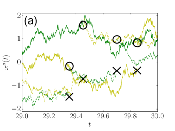
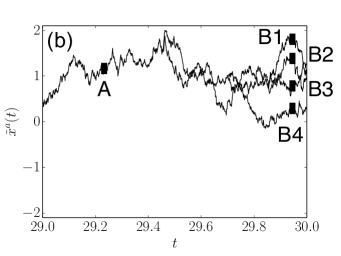
Figure 1: (Color online) (a) Trajectories $x^{a}(t)$ generated by population dynamics at fixed total population $N_{c}=4$ for the model system described in Section II.3 ($\epsilon=1,h=1$). The different colours or line types, which are the green (dark grey in the printed version) solid line, green dashed line, yellow (light grey in the printed version) solid line and yellow dashed line, represent different copies. At certain times, some copies of the system are removed ($\times$ symbols) and others are duplicated ($\circ$ symbols). The time interval $\Delta T$ for the cloning procedure is set to be 0.05, and the time step for solving the Langevin equation is 0.001 (See Appendix A.1 for the details of the algorithm). (b) Representative sample paths $\tilde{x}^{a}(t)$ for the distribution $P_{h}[X]$, derived from those in (a) by keeping only trajectories surviving up to final time $\tau=30$. For each cloning event, we also copy the history of the trajectory, which replaces the history of the eliminated trajectory. This means that the trajectories $(\tilde{x}^{a}(t))_{a=1}^{N_{c}}$ overlap, especially for early times. For example, in panel (b), the point A appears in the past of the four points B1,$\dots$,B4. For any point $x^{a}(t)$ (such as A,B1,B2,$\dots$), we define the multiplicity $m_{a}(t,\tau)$ as the number of trajectories that include this point, and survive until the final time $\tau$. So for point $A$, the multiplicity is $m_{a}(t,\tau)=4$ but for B1,$\dots$,B4 then $m_{a}(t,\tau)=1$. (For all points in the trajectories who die before $\tau$, which are not drawn in the panel (b), $m_{a}(t,\tau)=0$.)

II.3 Numerical example

To show the operation of the population dynamics method, we introduce a simple model of diffusion in a quartic potential. That is, $F(x)=-x^{3}$ and $B(x)=\sqrt{2\epsilon}$, where $\epsilon$ is the noise strength (or temperature). We take $\lambda_{\rm c}=0$ and $\lambda_{\rm d}=x(x+1)$. For $h<0$ the distribution $P_{h}$ is concentrated on trajectories with small values of $\lambda_{\rm d}$, which tend to localise near $x\approx-\frac{1}{2}$. Here we focus on the case $h>0$, which leads to unusually large values of $\lambda_{\rm d}$. Those can be realised either for $x>0$ or $x<0$ but at large $\tau$ this rare event is almost always realised by trajectories that have $x>0$ (as illustrated in Fig. 1). This simple problem can be solved exactly in the zero-noise limit (see Appendix D).

The operation of the population dynamics method is illustrated in Fig. 1. Fig. 1(a) shows four copies of the system that evolve in time, except that some trajectory segments stop and others branch, as the cloning operates. Fig. 1(b) shows four representative trajectories (sample paths) for the distribution $P_{h}[X]$, which have been reconstructed from panel (a), by tracing backwards in time from the clones that survived up to the final time $\tau$.

III Sampling errors within population dynamics

III.1 Distributions $p_{\rm end}$ and $p_{\rm ave}$

The accuracy of the population dynamics is limited by the number of clones $N_{c}$ used in its numerical implementation, as we now explain. Consider the distribution

$$p_{\rm ave}(x)=\lim_{\tau\rightarrow\infty}\Big{\langle}\tau^{-1}\!\int_{0}^{\tau}\delta(x_{t}-x)\mathrm{d}t\Big{\rangle}_{h},$$ (8)

which indicates the fraction of time spent at position $x$, within the biased ensemble. We also define

$$p_{\rm end}(x)=\lim_{\tau\rightarrow\infty}\left\langle\delta(x_{\tau}-x)\right\rangle_{h},$$ (9)

which indicates the fraction of trajectories for which the particle’s final position is $x$. For the stationary state of the dynamics (1), which corresponds to $h=0$, time-translational invariance ensures that $p_{\rm ave}=p_{\rm end}$. However, this is not the case for biased ensembles where $h\neq 0$, as illustrated in Populationdynamics ; garrahan2 and in Fig. 2.

The population dynamics method provides estimates of both $p_{\rm ave}$ and $p_{\rm end}$. Let the position of clone $a$ at time $t$ be $x^{a}(t)$, with $a=1\dots N_{c}$. Recalling Fig. 1(a), note that the functions $x^{a}(t)$ are not continuous in time and do not represent sample paths for the distribution $P_{h}[X]$. However, from the definition of the population dynamics algorithm (as explained in Appendix A.1), the distribution of $x^{a}(t)$ can be used to estimate $p_{\rm end}(x)$, as

$$p_{\rm end}(x)\simeq\frac{1}{\tau N_{c}}\int_{0}^{\tau}\sum_{a=1}^{N_{c}}\delta(x-x^{a}(t))\mathrm{d}t.$$ (10)

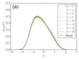
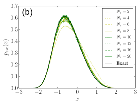
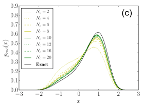
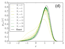
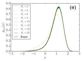
Figure 2: (Color online) (a-d) Distributions $p_{\rm end}(x)$ and $p_{\rm ave}(x)$, defined in (8) and (9), calculated from the population dynamics method, with various numbers of clones $N_{c}$. The different panels correspond to a different value of $h$ ($h=\pm 1$) or a different distribution function ($p_{\rm end}(x)$ or $p_{\rm ave}(x)$): (a) $p_{\rm end}(x)$ for $h=-1$, (b) $p_{\rm ave}(x)$ for $h=-1$ , (c) $p_{\rm end}(x)$ for $h=1$, and (d) $p_{\rm ave}(x)$ for $h=1$. For all panels, we set $\epsilon=1$ and $\tau=30$. The numerically exact result is plotted as a black line. We repeat the simulation $1200/N_{c}$ times and the result is the average of them (this procedure means that we vary $N_{c}$ while keeping a fixed computational cost). The results of the population dynamics converge to the analytical ones as $N_{c}$ increases. (e) $p_{\rm ave}(x)$ for $h=1$ (improved estimation) calculated from a population dynamics method with control-with-feedback, as described in Section IV.3 and Section V. Results are shown after two iterations of the feedback procedure. The exact distribution $p_{\rm ave}(x)$ is again shown as a black line. The comparison between (d) and (e) indicates that the convergence with respect to $N_{c}$ is improved significantly by the control-with-feedback method. The variance $m_{2}$ and the relative entropy $D_{2}$ defined in  (12) and (13) both measure how much large values of $N_{c}$ are required for the cloning procedure to be reliable. For the panel (b), (d) and (e), these values are ($m_{2}=0.068$, $D_{2}=0.039$), ($m_{2}=0.33$, $D_{2}=0.17$) and ($m_{2}=0.0064$, $D_{2}=0.0032$) respectively.

In order to construct sample paths, which we denote by ${\tilde{x}}^{a}(t)$, we trace backwards in time from the clones that survive up to $\tau$, as shown in Fig. 1(b). There are still $N_{c}$ paths ${\tilde{x}}^{a}$, but these overlap, particularly at early times. Since these trajectories correspond to $P_{h}[X]$, the distribution of ${\tilde{x}}^{a}$ gives an estimate of $p_{\rm ave}(x)$, as:

$$p_{\rm ave}(x)\simeq\frac{1}{\tau N_{c}}\int_{0}^{\tau}\sum_{a=1}^{N_{c}}\delta(x-{\tilde{x}}^{a}(t))\mathrm{d}t.$$ (11)

The approximate equalities in the relations (10) and (11) become exact in the limit $N_{c}\to\infty$ and $\tau\rightarrow\infty$, in which the population dynamics gives exact results.

We show numerical examples of these functions in Fig. 2, for a particle moving in a quartic potential, as introduced in Section II.3. We estimate $p_{\rm ave}$ and $p_{\rm end}$ from (10) and (11), and show them in Fig. 2. In the same figure, we also plot the numerically exact distributions, obtained by numerical solution of a modified Fokker-Planck equation (see Touchette and Appendix B.2). The population dynamics converges to the exact result as $N_{c}$ is increased. Also shown in Fig. 2 are results using the control-with-feedback method that we introduce in this paper: these results will be discussed in later sections.

III.2 Multiplicity

The population dynamics method gives accurate results in the limit of large $N_{c}$. The central idea is that in a large population, short-lived rare fluctuations will occur. Based on these short-lived fluctuations, we duplicate some of the clones: repeated application of this procedure generates the long-lived fluctuations that are relevant for large deviation theory. For this to be effective, the population on which the cloning operates must be large enough to capture the relevant short-lived fluctuations. That is, the cloning part of the algorithm can allocate extra statistical weight to configurations that are already present in the population, but new configurations are only generated by the natural (unbiased) dynamics of the system.

Assuming that $N_{c}$ is large enough for efficient operation of the algorithm, the configurations that are associated with long-lived dynamical fluctuations are distributed as $p_{\rm ave}$, but the cloning step operates on a population distributed as $p_{\rm end}$. From the argument above, it is clear that if typical samples from $p_{\rm ave}$ are rare with respect to $p_{\rm end}$, then a large population is required in order to obtain accurate results. To quantify this, it is useful to define the multiplicity $m_{a}(t,\tau)$ of clone $a$ at time $t$ as the number of its descendants that survive until the final time $\tau$ (see Fig. 1). Rewriting (8) as $p_{\rm ave}(x)\simeq\frac{1}{\tau N_{c}}\int_{0}^{\tau}\sum_{a=1}^{N_{c}}m_{a}(t,\tau)\delta(x-x^{a}(t))\mathrm{d}t$ and comparing with (9), one sees that for a clone with position $x=x^{a}(t)$, the expected value of its future multiplicity is $p_{\rm ave}(x)/p_{\rm end}(x)$. Since the clone positions $x^{a}(t)$ are distributed as $p_{\rm end}$, averaging this future multiplicity over configurations $x$ yields $\int p_{\rm end}\cdot(p_{\rm ave}/p_{\rm end})\mathrm{d}x=\int p_{\rm ave}(x)\mathrm{d}x=1$, which reflects the fact that the population size is constant in time.

In practice, the distribution of the multiplicity $m_{a}(t,\tau)$ is very broad, and typical multiplicities are far from their average values. There are many clones for which no descendants survive until time $\tau$ (see Fig. 1(a)), in which case $m_{a}(t,\tau)=0$. In order to maintain an average multiplicity of $1$, these zero-multiplicity clones are balanced by a small number of clones with larger multiplicity. It is useful to define $\tilde{N}_{c}(t,\tau)$ as the number of clones that are present in the population at time $t$, for which $m_{a}(t,\tau)>0$. Numerical results for $\tilde{N}_{c}(t,\tau)$ are shown in Fig. 3 – this quantity decreases rapidly as $t$ decreases away from $\tau$, showing that many clones have no surviving descendants: it follows that the multiplicities of the surviving clones must be large. From (11), one sees that if $\tilde{N}_{c}(t,\tau)$ is small, numerical estimates of $p_{\rm ave}$ contain only a small number of independent samples, which can lead to large numerical uncertainties within the algorithm.

Moreover, the presence of large multiplicities within the cloning scheme can lead to large systematic errors, which cannot be reduced by averaging over repeated runs of the same algorithm. On running the system with a fixed population, the future multiplicity of any clone is bounded above by the population size $N_{c}$. We will show in the next section that this constraint has serious implications for systems in the small noise limit. More generally, in order to characterise whether a system requires a large population or not, it is useful to define two numbers that measure how different are the distributions $p_{\rm ave}$ and $p_{\rm end}$. These are

$$m_{2}=\int p_{\rm end}(x)\left[\left(\frac{p_{\rm ave}(x)}{p_{\rm end}(x)}\right)^{2}-1\right]\mathrm{d}x$$ (12)

and

$$D_{2}=\int p_{\rm ave}(x)\log\left(\frac{p_{\rm ave}(x)}{p_{\rm end}(x)}\right)\mathrm{d}x.$$ (13)

Given that $p_{\rm ave}(x)/p_{\rm end}(x)$ is the expected future multiplicity of a clone at $x$, we recognise $m_{2}$ as the variance of this multiplicity, with respect to the distribution $p_{\rm end}$ of clone positions (recall that the average multiplicity with respect to this distribution is equal to unity). Similarly $D_{2}$ is the relative entropy of $p_{\rm ave}$ with respect to $p_{\rm end}$ footnote:KullbackLeibler : this is related to the controlling forces that will be introduced in Section IV. Large values of $m_{2}$ and $D_{2}$ indicate that $p_{\rm end}$ and $p_{\rm ave}$ are different from each other, in which case larger values of $N_{c}$ will be required for accurate results within population dynamics. For the two cases $h=\pm 1$ shown in Fig. 2, we have for $h=-1$ that $(m_{2},D_{2})=(0.068,0.039)$ while for $h=+1$, $(m_{2},D_{2})=(0.33,0.17)$, reflecting the larger populations required for accurate results when $h=+1$. Obtaining general estimates of the actual population size $N_{c}$ required for convergence is an important goal for future work.

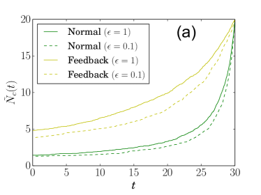
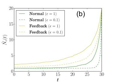
Figure 3: (Color online) The number of independent (distinct) clones $\tilde{N}_{c}(t)$ obtained from the normal population dynamics method (green line or dark grey line in the printed version) for $h=-1$ (a) and $h=1$ (b). The line type corresponds to the value of noise intensity: $\epsilon=1$ (solid line) and $\epsilon=0.1$ (dashed line). We set $N_{c}=20$ and $\tau=30$. When the distributions $p_{\rm ave}$ and $p_{\rm end}$ are very different from each other, we expect that $\tilde{N}_{c}(t)$ decreases rapidly as $t$ decreases from $\tau$: to illustrate this, note that (for $\epsilon=1$) $m_{2}=0.068$ for $h=-1$ and $m_{2}=0.33$ for $h=1$: the same ordering is preserved for smaller $\epsilon$. We also plot $\tilde{N}_{c}(t)$ obtained from the controlled population dynamics (yellow line or light grey line in the printed version) with the control-with-feedback explained in Section IV.3 and Section V. The larger values of $\tilde{N}_{c}(t)$ obtained with the control-with-feedback method lead to smaller statistical uncertainties in the results.

III.3 Sampling problems for weak noise

The effect described in the previous section is particularly severe for systems where the random (noise) force in (1) is small. To illustrate this case, we set $B(x)=\sqrt{2\epsilon}B_{0}(x)$, consistent with the numerical example of Sec. II.3 (for which $B_{0}=1$). The small noise limit is then $\epsilon\to 0$. We define $x^{*}=\operatorname*{arg\,max}_{x}[p_{\rm ave}(x)]$ as the most likely value of $x$, within the distribution $p_{\rm ave}$. The population dynamics requires that the typical multiplicity of a clone with position $x^{*}$ should be (at least) of order $m^{*}\equiv p_{\rm ave}(x^{*})/p_{\rm end}(x^{*})$. This clearly cannot be achieved unless $N_{c}\gtrsim m^{*}$, which provides an estimate of the number of clones required for accurate results.

This multiplicity $m^{*}$ increases exponentially as the noise intensity of the system becomes small. In this limit, the dynamics of the system runs increasingly slowly so it is natural to rescale either the time variable or (equivalently) the biasing field $h$ as $\tilde{G}(\tilde{h})\equiv\epsilon G(h)$ with $\tilde{h}\equiv h\epsilon$. (This scaling also appears in the hydrodynamic limit of microscopic models Kipnis_Landim .) In this limit, $p_{\rm ave}$ and $p_{\rm end}$ satisfy a large deviation principle with respect to the noise intensity $\epsilon$: $p_{\rm ave}(x)\sim\mathrm{e}^{-I_{\rm ave}(x)/\epsilon}$ and $p_{\rm end}(x)\sim\mathrm{e}^{-I_{\rm end}(x)/\epsilon}$. Hence, $m^{*}\sim\mathrm{e}^{I_{\rm end}(x^{*})/\epsilon}$, where we used $I_{\rm ave}(x^{*})=0$. This indicates that we need an exponentially large $N_{c}$ as $\epsilon$ becomes small. More quantitatively, we define a characteristic noise intensity $\epsilon^{*}$ by

$$\epsilon^{*}\equiv\frac{1}{I_{\rm end}(x^{*})}.$$ (14)

For $\epsilon<\epsilon^{*}$, we expect that population dynamics can not be used practically, because of the exponentially large $N_{c}$ required.

As a numerical example, we again consider the Brownian particle introduced in Section II.3. We numerically estimate $\epsilon^{*}$ by using a quadratic approximation of the large deviation function $I_{\rm end}(x)$. We plot it as a green vertical line in Fig. 4. In the same figure, we show the result of the population dynamics for $\tilde{G}(\tilde{h})$ as $\epsilon$ is reduced, with a red constant line corresponding to the analytical value of $\tilde{G}(\tilde{h})$ in the $\epsilon\rightarrow 0$ limit (See Appendix D.3 for its determination). Below the characteristic value $\epsilon^{*}$, the population dynamics method converges very poorly as $N_{c}$ increases.

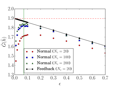
Figure 4: (Color online) Estimates of $\tilde{G}(\tilde{h}=1)$, as $\epsilon$ is varied. We compare results from the normal population dynamics and from the control-with-feedback method explained in Section IV.3 and Section V. The analytical result for $\lim_{\epsilon\rightarrow 0}\tilde{G}(\tilde{h})$ is shown as a red dashed line, and the characteristic value of the noise intensity $\epsilon^{*}$, defined in (14), is plotted as a green vertical solid line. The standard method fails for $\epsilon$ smaller than $\epsilon^{*}$ but the control-with-feedback method (black continuous line and black circles) converges to the correct value even for $\epsilon<\epsilon^{*}$.

IV Population dynamics with a feedback control

IV.1 Controlled dynamics

To resolve the sampling issues described in the previous section, we introduce a “control strategy”, which modifies the original model (1), in order to make the rare events of interest more likely. (These large deviation problems have dual representations in terms of optimal control problems OptimalControlFleming ; jack15-epj ; chetrite15-jstat ; fleming92 ; hartmann12 ; kappen13 , which provide a natural interpretation of the method presented here.) The modified model is

$$\dot{x}_{t}=F(x_{t})+w(x_{t})+B(x_{t})\xi_{t},$$ (15)

where $w(x)$ is a controlling force which we write as

$$w(x)=h\kappa\lambda_{c}(x)-\kappa\nabla V(x),$$ (16)

where $V$ acts as a potential. A straightforward calculation shows that averages with respect to the biased distribution $P_{h}$ can be rewritten as averages with respect to this modified dynamics, but with a bias on a different observable $\Lambda^{w}$, which replaces $\Lambda$. That is, by defining

$$\Lambda^{w}=\frac{1}{\tau}\int_{0}^{\tau}\lambda^{w}(x_{t})\mathrm{d}t$$ (17)

with

$$\lambda^{w}=\lambda_{\rm d}+\frac{1}{h}[(F+w/2)\cdot\kappa^{-1}w-\tfrac{1}{2}\mathrm{Tr}(H_{V}\kappa)],$$ (18)

in which $H_{V}$ is a Hessian matrix with elements $(\partial^{2}V/\partial x_{i}\partial x_{j})$, we have

$$P_{h}[X]=P_{w}[X]\mathrm{e}^{V(x_{\tau})-V(x_{0})}$$ (19)

with

$$P_{w}[X]=\pi_{0}(x_{0})\exp\!\Big{[}\!-\!\!\int_{0}^{\tau}\!\!\!{\cal L}^{w}(x_{t},\dot{x}_{t})\mathrm{d}t+h\tau\Lambda^{w}(\tau)\Big{]},$$ (20)

where ${\cal L}^{w}$ is the action corresponding to the controlled Langevin equation (15) obtained by replacing $F\mapsto F+w$ in (6). See Appendix B for details of the derivation. We stress that these relations are satisfied for any control $w$.

Averages with respect to $P_{w}$ are denoted by $\langle\cdot\rangle_{w}$, and can be calculated using the population dynamics method with the modified model (15). Physically, equation (19) says that rare events for the system (1) have an alternative characterisation as rare events for the controlled system (15). More precisely, from (19), the averages $\langle\cdot\rangle_{h}$ and $\langle\cdot\rangle_{w}$ are not equal, but their associated probability distributions differ only through boundary terms at initial and final times. For large $\tau$, we focus on properties far from initial and final times, in which case the averages $\langle\cdot\rangle_{h}$ and $\langle\cdot\rangle_{w}$ are equivalent. This equivalence implies that

$$p_{\rm ave}^{w}=p_{\rm ave},$$ (21)

where $p_{\rm ave}^{w}$ is defined as in (8) but for the controlled population dynamics (15). On the other hand, when we consider properties close to the final time $\tau$ (which are not relevant for the large deviations of time-averaged quantities), the two averages $\langle\cdot\rangle_{h}$ and $\langle\cdot\rangle_{w}$ are different in general. For example, the end-time distribution $p_{\text{end}}^{w}$ for the controlled dynamics differs from its uncontrolled counterpart as

$$p_{\rm end}^{w}\propto p_{\rm end}\mathrm{e}^{-V(x)},$$ (22)

as read from (19) (or see Appendix B.2 for a detailed derivation of (21) and (22)). Thus the control $w$ allows $p_{\rm end}^{w}$ to be varied, while always keeping $p_{\rm ave}^{w}$ constant (and hence leaving unchanged the bulk properties of $P_{h}$, which are relevant for the large deviations of time-averaged quantities).

IV.2 Optimal control

These results apply for any control force $w$, but a (unique) optimal choice $w^{*}$ can be defined by the condition

$$p_{\rm ave}^{w^{*}}=p_{\rm end}^{w^{*}}.$$ (23)

From (12,13), this result implies that for the controlled population dynamics, $m_{2}=D_{2}=0$: all clones have expected future multiplicity of unity, regardless of their position. In fact, this case also implies that $\lambda^{w^{*}}(x)$ is independent of $x$ (see Appendix B.2), so that there is no cloning or deletion of clones in the optimally-controlled population dynamics algorithm. That is, all multiplicities are equal to unity (not just their expected values). The result is that the optimally-controlled process jack15-epj ; chetrite15-jstat ; fleming92 ; hartmann12 ; kappen13 generates directly the path measure $P_{h}$, up to the corrections given in (19) Evans ; JackSollich ; NemotoSasa2 ; maes08 ; Chetrite_Touchette2 . Note also that $D_{2}$, as defined in (13) for the original population dynamics, is also related to an average of the optimal control potential $V^{*}$ (where $V^{*}$ is the potential $V$ corresponding to the optimal control $w^{*}$), since $\log[p_{\rm ave}(x)/p_{\rm end}(x)]=-V^{*}(x)-\log[\int\mathrm{e}^{-V^{*}(x^{\prime})}p_{\rm end}(x^{\prime})\mathrm{d}x^{\prime}]$.

The optimal control can be estimated by using the population dynamics with any non-optimal control force $w$ (or its corresponding potential $V$). We perform the population dynamics and generate sample paths from $P_{w}$. From the definition of the optimal force (23) with the relations between $p_{\rm end,ave}^{w}$ and $p_{\rm end,ave}$ (21), (22), we obtain

$$V^{*}(x)=V(x)+\log\frac{p^{w}_{\rm end}(x)}{p^{w}_{\rm ave}(x)}.$$ (24)

Since all terms on the right-hand side of (24) can be measured from the population dynamics with a non-optimal control $w$, this allows an estimate of $V^{*}$, and hence of $w^{*}$.

IV.3 Control-with-feedback for population dynamics

Based on (24), we arrive at the following iteration and feedback scheme for efficient analysis of large deviations of $\Lambda(\tau)$. Starting with the original population dynamics of Populationdynamics , we obtain estimates $p_{\rm end}^{0}$ and $p_{\rm ave}^{0}$ of $p_{\rm end}$ and $p_{\rm ave}$, and we use (24) to obtain an estimate of the optimal control potential $V^{*}$, which we denote by $V^{1}$. We then repeat the population dynamics calculation with a control force $w=w^{1}$ derived from the potential $V^{1}$. We use results from this new calculation together with (24) to obtain a new (more accurate) estimate of the optimal control. Iterating this scheme, the estimate of $V^{*}$ at iteration $r$ is $V^{r}$. As $V^{r}\to V^{*}$, we have from (24) that $p^{w}_{\rm end}\to p^{w}_{\rm ave}$, and hence the sampling problems described in Sec. III.2 are reduced. This improves the accuracy of the population dynamics method.

Given sufficiently many clones $N_{c}$, the original method of Populationdynamics can already provide accurate results, but we have demonstrated that for finite $N_{c}$ there may be large systematic errors. The strength of our scheme is that on repeated iteration, the control potential $V$ approaches the optimal control $V^{*}$, and the errors within the method are reduced. Thus, the numerical accuracy of the method increases as the scheme is iterated.

For the implementation of this iteration scheme, we require a computational representation of the function $V(x)$, and its gradient $\nabla V$. From (24), a natural choice might be to represent $p_{\rm ave}$ and $p_{\rm end}$ by histograms, based on a discretisation of the configuration space. However, this choice does not facilitate estimation of $\nabla V$, and it is also unfeasible in high-dimensional systems. We therefore use a potential $V$ that is defined in terms of a set of basis functions $\zeta_{i}$, with coefficients $c_{i}$:

$$V(x)=\sum_{i=1}^{k}c_{i}\zeta_{i}(x).$$ (25)

where $k$ is the size of the basis set.

At stage $r$ of our iterative scheme, the coefficients $c$ are denoted by $\bm{c}^{r}=(c^{r}_{i})_{i=1}^{k}$. In the absence of prior information about the optimal control $V^{*}$, the first stage of the method ($r=0$) uses the original population dynamics, so $c_{i}^{0}=0$ for all $i$. In stage $r+1$, we update these coefficients according to (24) so that the potential $V^{r+1}$ in the next stage is the best available estimate of $V^{*}$. There is considerable freedom in how to obtain this estimate: we take

$$\bm{c}^{r+1}={\rm argmin}_{\bm{c}}\int_{\Omega_{r}}\Bigg{[}V^{r}(x)+\log\frac{p^{w,r}_{\rm end}(x)}{p^{w,r}_{\rm ave}(x)}\\ -\sum_{i=0}^{k}c_{i}\zeta_{i}(x)\Bigg{]}^{2}\mathrm{d}x,$$ (26)

where $p^{w,r}_{\rm end}$ is the numerical estimate for $p^{w}_{\rm end}$ obtained at iteration $r$, and similarly $p^{w,r}_{\rm ave}$. The state space $\Omega_{r}$ is defined as the space where $p^{w,r}_{\rm ave}>0$ (note that $p^{w,r}_{\rm end}(x)>0$ whenever $p^{w,r}_{\rm ave}(x)>0$, from the definition of how to construct $\tilde{x}^{a}(t)$ as shown in Fig. 1(b)).

We emphasise that, for any basis set $\zeta_{i}$ (with any truncation number $k$), eq. (19) is satisfied, meaning that if the number of clones $N_{c}$ and the time $\tau$ are large enough, the result of any controlled population dynamics always leads to the same results, which can also be obtained from the original (uncontrolled) population dynamics. However, the choice of the expansion functions $\zeta_{i}(x)$ (and the value of the truncation number $k$) does affect the computational cost, through the number of clones required for convergence, as discussed in Section III.2.

IV.4 Advantages of the control-with-feedback for population dynamics, and relation to other methods

Compared to the original population dynamics method, the addition of control forces and the use of iteration and feedback increase the complexity of the method presented here. Here, we summarise the improvements that these changes achieve. Typically, existing methods either exploit an ensemble (population) of copies of the system DMC ; Aldous ; Grassberger ; Lelievre ; Garnier ; Rolland , or they use modified (controlled) dynamical rules to drive the system towards rare events of interest Nemoto_Sasa_PRL ; Berg_Neuhaus1 ; Wang_Landau1 ; OrtizLaelbling ; DupuisWang ; CappeDoucGuillin ; ChanLai ; hartmann12 , or they use path-sampling methods Hedges ; speck12 . All these methods are useful, but the population-based methods can suffer convergence problems, due to the very large populations required in some problems. On the other hand, the controlled methods require accurate estimation of an optimal control force that is typically a high-dimensional and complex object, which can be difficult to represent computationally (see for example JackSollich2 ). Path sampling methods are most effective when the ensemble $P_{h}$ has time-reversal symmetry, which limits their applicability in non-equilibrium settings. The method proposed here is a mixture of the population-based and control-based methods, as illustrated schematically in Fig 5.

In terms of the applicability of this new method, we expect the following general behaviour. For complex high-dimensional problems, accurate representation of the optimal control $V^{*}$ is likely to be difficult, but we expect even approximate representations of $V^{*}$ to significantly improve the performance of the population dynamics method. Thus, the controlled method should reduce the computational cost of problems that are already tractable using population dynamics, allowing access (for example) to larger system sizes and larger values of the bias parameter $h$. On the other hand, for relatively simple problems such as the particle in a quartic potential of Sec. II.3, the original population dynamics fails for small noise (Fig. 2) but we would expect that a solution by the controlled method of Nemoto_Sasa_PRL might already be possible. However, for a similar model in three or more dimensions, we expect that the method of Nemoto_Sasa_PRL would already be challenging, due to the difficulty of representing exactly the effective potential. Here, we combine that control strategy with population dynamics: we arrive at a flexible method that exploits the strengths of both approaches, and which we anticipate will be effective in a wide variety of problems.

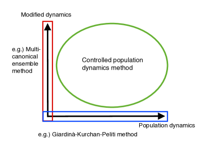
Figure 5: (Color online) A schematic map illustrating the methodological situation of the controlled population dynamics.

V Numerical example

To illustrate the control-with-feedback method, we consider the numerical example from Section II.3, and we take the effective description in (25) to be a quartic polynomial: $\zeta_{i}(x)\equiv x^{i}$ (that is, “$x$ raised to the power $i$”) and $k=4$. For the first iteration of the method we take $(c_{i}^{0})_{i=1}^{k}=0$. Note that this potential-parametrisation of $V$ cannot capture the exact $V^{*}$, neither for $\epsilon>0$ nor in the limit $\epsilon\rightarrow 0$ (see Appendix D). This emphasises that the control-with-feedback method does not require a perfect representation of the optimal control in order to improve the convergence of the population dynamics method.

Fig. 2 shows estimates of the distribution $p_{\rm ave}$ obtained using the original cloning method (Fig. 2(a-d)), compared with the results obtained using control-with-feedback procedure proposed here (Fig. 2(e)). (Two iterations of the feedback were used, which allow an accurate estimate of the optimal control potential $V^{*}$.) The comparison between Fig. 2(d) and Fig. 2(e) shows that the number of clones required to obtain convergence to the exact result is much reduced using the control-with-feedback method.

In the weak-noise limit $\epsilon\rightarrow 0$, one can see this advantage more clearly. In this limit, a sampling issue arises because of the exponential increase of the required number of copies $N_{c}$, as discussed in Section III.3. Fig. 3(a) shows numerical results for $\tilde{G}(\tilde{h})$, as $\epsilon$ is reduced. The normal population dynamics converges very poorly for small noise, $\epsilon<\epsilon^{*}$. However, the controlled population dynamics does not fail at small $\epsilon$ because it maintains $p^{w}_{\rm end}\approx p_{\text{ave}}^{w}$ footnotecitation_anneaing .

We then consider statistical errors. Fig. 3(b) shows the number of distinct clone positions in the population, $\tilde{N}_{c}(t)$. Again, the control-with-feedback method performs better than the original method, in that it averages over a larger sample of distinct positions, reducing the statistical errors.

Finally, in order to illustrate how the control-with-feedback method improves the standard population dynamics method, in Fig. 6, we show the integrands of $m_{2}$ and $D_{2}$ defined in (12) and (13) footnote:m2andD2 . As discussed in Section III.2 and Section III.3, the standard population dynamics has sampling issues, which are captured by the deviations of $m_{2}$ and $D_{2}$ from 0. In the figure, we can see that the control-with-feedback method greatly reduces the values of $m_{2}$ and $D_{2}$ close to 0, ensuring that $p_{\rm end}^{w}$ and $p_{\rm ave}$ are closer than in the original cloning, thus yielding better performances as seen throughout this section.

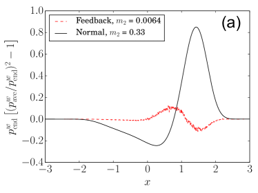
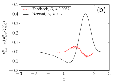
Figure 6: (Color online) The integrands of $m_{2}$ and $D_{2}$ defined as (a) $p_{\rm end}^{w}(x)\left[\left(\frac{p_{\rm ave}^{w}(x)}{p_{\rm end}^{w}(x)}\right)^{2}-1\right]$ and (b) $p_{\rm ave}^{w}(x)\log\left(\frac{p_{\rm ave}^{w}(x)}{p_{\rm end}^{w}(x)}\right)$, (see (12) and (13)), for the standard (normal) population dynamics method ($w=0$) and for the control-with-feedback method ($w$: obtained from the control-with-feedback method)). For the control-with-feedback method, we set $N_{c}=20$. In the legends of the figures, we put the values corresponding to $m_{2}$ and $D_{2}$.

VI Outlook

We have shown that the performance of the population dynamics algorithm for sampling large deviations Populationdynamics can be improved by introducing a controlling force $w$. Given the optimal choice for this force, the rare events of interest in large deviation theory can be characterised as typical trajectories of the controlled system without any cloning. In complex systems with many degrees of freedom it is likely that the optimal $w$ cannot be determined exactly, but even non-optimal controls can still significantly improve both the statistical and the systematic errors associated with the population dynamics method (see Section V). It is straightforward to improve existing population dynamics codes to include this approach: we expect that it will significantly expand the range of systems for which numerical calculations can be performed, including open quantum systems Garrahanquantum ; QuantumGarrahan , or more complex molecular dynamics models than those considered so far Hedges ; speck12 .

Appendix A Population dynamics method

In this appendix, complementing Section II.2 and Section III.1, we explain the details of the population dynamics algorithm.

A.1 Population dynamics algorithm

The population dynamics is a numerical technique designed to evaluate a large deviation function associated to the cumulant generating function (CGF) of a time-averaged observable $\Lambda(t)$. Each step of the algorithm consists of a first sub-step in which the normal (unbiased) dynamics of the system is simulated for a time $\Delta T$, followed by an elimination-multiplication sub-step. (The elimination-multiplication sub-step is also called a cloning step, or a mutation-selection step.) In detail, the method is:

1. Generate $N_{c}$ initial conditions, for example, drawn from the stationary state of the unbiased ($h=0$) dynamics.

2. Repeat the following procedure $M$ times. (The iteration index is $m=0,1,\dots,M-1$.)

   1. For each copy of the system, perform the normal dynamics from $t=m\,\Delta T$ to $(m+1)\Delta T$. We denote each trajectory by $x^{a}(t)$. (Throughout this section, $a=1,2,....,N_{c}$.) During the simulation, for each trajectory, calculate

      $$s_{a}=\exp\Big{\{}h\left[(t+\Delta T)\,\Lambda(t+\Delta T)-t\Lambda(t)\right]\Big{\}}.$$ (27)

   2. For each trajectory $a$, calculate an integer $n_{a}$ as

      $$n_{a}=\left\lfloor\frac{s_{a}}{\sum_{b}s_{b}}N_{c}+\eta\right\rfloor,$$ (28)

      where $\eta$ is a random number uniformly distributed on [0,1] and $\lfloor\cdot\rfloor$ denotes the lower integer part. Calculate and store the quantity $S_{m}=\sum_{b}s_{b}$.

   3. Multiply or eliminate each trajectory $a$ so that it appears $n_{a}$ times in the new population. (For example, if $n_{a}=0$ then trajectory $a$ is deleted. If $n_{a}=5$ then we retain trajectory $a$ and we introduce 4 new copies of that trajectory.)

   4. Eliminate or multiply trajectories within the population, chosen randomly and uniformly, so that the total number of surviving trajectories is $N_{c}$.

   5. Go back to (a), using the current set of configurations $x^{a}((m+1)\Delta T)$ as initial conditions for the next iteration of the normal dynamics.

Note that if the population were not kept constant in step 2c above, then the population would expand by a factor of $S_{m}/N_{c}$. It follows that the CGF can be estimated as

$$G(h)\simeq\frac{1}{M\,\Delta T}\sum_{m}\log\frac{S_{m}}{N_{c}}.$$ (29)

Also, averages over the population at the final time $\tau$ are estimates of averages with respect to $p_{\rm end}$:

$$\int f(x)p_{\rm end}(x)\mathrm{d}x\simeq\frac{1}{N_{\rm c}}\sum_{a=1}^{N_{\rm c}}f(x^{a}(\tau)),$$ (30)

which follows from the definition of $p_{\rm end}$. When estimating $p_{\rm end}$, we can improve the statistics by using the history of $x^{a}(t)$. That is, assuming an ergodicity property, we can replace $f(x^{a}(\tau)))$ by its time average, leading to

$$\int f(x)p_{\rm end}(x)\mathrm{d}x\simeq\frac{1}{\tau N_{\rm c}}\int_{0}^{\tau}\sum_{a=1}^{N_{\rm c}}f(x^{a}(t))\mathrm{d}t.$$ (31)

This means that the empirical distribution of $x_{a}(t)$ is an estimator for $p_{\rm end}$, as announced in (10).

In order to generate the sample paths corresponding to the biased measure $P_{h}$, we also need to copy the history of trajectory (not just the current configuration of $x$) in the selection-mutation procedure in step 2.(b) of the algorithm. This fact is directly derived from the definition of $P_{h}$. Thus, the $x^{a}(t)$ defined above do not correspond to sample paths of $P_{h}$. The paths are obtained as $\tilde{x}^{a}(t)$, which are defined as those trajectories that survive until the final time $\tau$ (see Fig. 1). In numerical simulations, there are several ways to generate (or reconstruct) these trajectories, as we now explain.

A.2 Generating continuous sample paths $\tilde{x}^{a}(t)$ for the biased dynamics

A simple way to characterise $\tilde{x}^{a}(t)$ is the following: If we do not require full sample paths but only wish to evaluate the biased average of an additive observable $A(\tau)=\int_{0}^{\tau}a(x(t))\,\mathrm{d}t$, a simple method Julien_Vivien consists in attaching a value of the observable $A$ to every trajectory and, at every time step, to update its value and copy/delete it together with the trajectory. Then, an evaluation of the biased average of $A$ is given by an average of the numerical values of $A$: this average runs over all trajectories that are present at the final time. For example, when we divide the configuration space into small bins and take $a_{i}(x(t))=1$ if $x(t)$ is in bin $i$, $A_{i}(\tau)/\tau$ is an estimate of $p_{\rm ave}$, integrated across the $i$th bin.

For the small systems where we can store all of the trajectories in the population dynamics, we can generate full sample paths corresponding to $\tilde{x}^{a}$. The procedure is as follows: we first generate all the trajectories, and then select those that survive until the final time $\tau$. Considering the $N_{c}$ copies at final time, indexed by $1\leq a\leq N_{c}$, one can follow the ancestors of every copy. Upon every coalescence observed backwards in time (corresponding to multiplications of clones in the original forwards simulation), one increments a counter $m_{a}(t,\tau)$ by the number of trajectories which have coalesced. At the end of the procedure, the counters $(m_{a}(t,\tau))_{1\leq a\leq N_{c}}$ represent, at time $t$, the number of descendants of a copy $a$ at final time $\tau$.

Appendix B Derivation of the ratio of path probability density (19)

In this appendix, complementing Section IV we derive the relation between $P_{h}[X]$ and $P_{w}[X]$, eq.(19). We show the derivation in two ways, one based on path probability densities (stochastic differential equations) and the other on Fokker-Plank equations.

B.1 Derivation using path probability density

We denote a trajectory of the system by $X=(x(t))_{0\leq t\leq\tau}$. From the definitions of $P_{h}[X]$ and $P_{w}[X]$, we have

$$\frac{P_{w}[X]\mathrm{e}^{-h\tau\Lambda^{w}(\tau)}}{P_{h}[X]\mathrm{e}^{-h\tau\Lambda(\tau)}}=\exp\Bigg{[}\int_{0}^{\tau}\left(\dot{x}-F\right)\cdot\kappa^{-1}w\mathrm{d}t\\ -\frac{1}{2}\int_{0}^{\tau}w\cdot\kappa^{-1}w\mathrm{d}t\Bigg{]}$$ (32)

The integrand on the right-hand side is written as

$$\left(\dot{x}-F\right)\cdot\kappa^{-1}w-\frac{1}{2}w\cdot\kappa^{-1}w\\ =\dot{x}\cdot\left(-\nabla V+h\lambda_{\rm c}\right)-\left(F+\frac{1}{2}w\right)\cdot\kappa^{-1}w,$$ (33)

where we have used the expression of $w(x)$ as given in the main text ($w(x)=\kappa\left[-\nabla V(x)+h\lambda_{\rm c}(x)\right]$). We then consider the integral of the first term on the right hand side:

$$\int_{0}^{\tau}\dot{x}\cdot\left(-\nabla V\right)\mathrm{d}t.$$ (34)

Since the trajectory $X$ is generated from the stochastic differential equation (15) and we use the Itō convention, the time-derivative of $V(x(t))$ is given by Itō’s formula

$$\frac{\mathrm{d}}{\mathrm{d}t}V=\dot{x}\cdot\nabla V+\frac{1}{2}{\rm Tr}\left[B^{T}H_{V}B\right].$$ (35)

Here $H_{V}$ is a Hessian matrix defined as $(H_{V})_{i,j}=\frac{\partial V}{\partial x_{i}\partial x_{j}}$. Combining (35,34) we have

$$\int_{0}^{\tau}\dot{x}\cdot\left(-\nabla V\right)\mathrm{d}t=-V(x(\tau))+V(x(0))\\ +\int_{0}^{\tau}\frac{1}{2}{\rm Tr}\left[B^{T}H_{V}B\right]\mathrm{d}t.$$ (36)

Thus, from (32), (33) and (36), we get

$$\frac{P_{w}[X]\mathrm{e}^{-h\tau\Lambda^{w}(\tau)}}{P_{h}[X]\mathrm{e}^{-h\tau\Lambda(\tau)}}=\mathrm{e}^{-V(x(\tau))+V(x(0))}\\ \times\exp\Bigg{\{}\int_{0}^{\tau}\Big{[}\frac{1}{2}{\rm Tr}\left[B^{T}H_{V}B\right]+h\dot{x}\cdot\lambda_{\rm c}\\ -\left(F+\frac{w}{2}\right)\cdot\kappa^{-1}w\Big{]}\mathrm{d}t\Bigg{\}}$$ (37)

Finally, by noticing ${\rm Tr}\left[B^{T}H_{V}B\right]={\rm Tr}\left[H_{V}\kappa\right]$ and using the definitions of $\Lambda^{w}$ and $\Lambda$, the right hand side is $\mathrm{e}^{-V(x(\tau))+V(x(0))}\mathrm{e}^{h\tau\Lambda(\tau)-h\tau\Lambda^{w}(\tau)}.$ Hence one arrives at Eq. (19).

B.2 Derivation using time-evolution operator

An alternative derivation of (19) is obtained by using a ‘tilted’ generator (or master operator) for the biased ensemble of trajectories. Let $u^{h}(x,\tau)$ be the (unnormalised) probability density at time $\tau$, obtained as a marginal of the path distribution $P_{h}$. As discussed, for example, in Appendix A.2 of Chetrite_Touchette2 , this distribution evolves in time according to a generalised Feynman-Kac formula as

$$\frac{\partial}{\partial\tau}u^{h}=L^{h}[u^{h}],$$ (38)

with

$$\begin{split}L^{h}[f]\equiv&L_{\rm FP}^{F}[f]+h\left(\lambda_{\rm d}+\lambda_{\rm c}\cdot F\right)f\\ &+\frac{h^{2}}{2}\left(\lambda_{\rm c}\cdot\kappa\lambda_{\rm c}\right)f-h\nabla\cdot\left(\kappa\lambda_{\rm c}f\right).\end{split}$$ (39)

Here, the Fokker-Planck operator $L_{\rm FP}^{F}$ is

$$L_{\rm FP}^{F}[f]=-\nabla\cdot\left[Ff\right]+\frac{1}{2}\sum_{i,j}\frac{\partial^{2}}{\partial x_{i}\partial x_{j}}\kappa_{ij}f,$$ (40)

where the superscript $F$ on $L_{\rm FP}^{F}$ indicates that the particle feels the physical force $F$ introduced in (1).

For the controlled population dynamics, the analogue of $u^{h}$ is $u^{w}(x,\tau)$, which evolves as $\frac{\partial}{\partial\tau}u^{w}=L^{w}[u^{w}]$, with

$$L^{w}[f]\equiv L_{\rm FP}^{F+w}[f]+h\lambda^{w}f.$$ (41)

The relation (19) follows from a duality relation between $L^{h}$ and $L^{w}$:

$$L^{h}[f]=\mathrm{e}^{V}L^{w}[f\mathrm{e}^{-V}].$$ (42)

This relation may be verified directly from (39,41), noting that the potential $V$ is related to the control $w$ via the definition $w=h\kappa\lambda_{\rm c}-\kappa\nabla V$.

From (38), we note that the operator $U^{h}_{\tau}=\mathrm{e}^{\tau L^{h}}$ corresponds to integration forward in time over a duration $\tau$. Similarly $U^{w}_{\tau}={\rm e}^{\tau L^{w}}$, and from (42) we have $U^{h}_{\tau}[f]=\mathrm{e}^{V}U^{w}_{\tau}[f\mathrm{e}^{-V}]$. Setting $f(x)=\delta(x-x_{0})$, then $u^{h}(x,\tau|x_{0},0)=U^{h}_{\tau}[f]$ is the (unnormalised) probability density at $x$, for a particle that was at $x_{0}$ a time $\tau$ earlier. Defining similarly $u^{w}(x,\tau|x_{0},0)$, (42) implies

$$u^{h}(x,\tau|x_{0},0)=\mathrm{e}^{V(x)}u^{w}(x,\tau|x_{0},0)\mathrm{e}^{-V(x_{0})}.$$ (43)

Hence one arrives at (19) of the main text.

This approach also provides insight into the distributions $p_{\rm ave}$ and $p_{\rm end}$, as discussed in Populationdynamics ; JackSollich . One easily sees that

$$p_{\rm end}(x)=\lim_{\tau\to\infty}\frac{u^{h}(x,\tau|x_{0},0)}{\int_{x^{\prime}}u^{h}(x^{\prime},\tau|x_{0},0)},$$ (44)

which is independent of $x_{0}$. Similarly,

$$p_{\rm ave}(x)=\lim_{\tau\to\infty}\frac{\int_{x_{1}}u^{h}(x_{1},\tau/2|x)u^{h}(x,0|x_{0},-\tau/2)}{\int_{x^{\prime},x_{1}}u^{h}(x_{1},\tau/2|x^{\prime})u^{h}(x^{\prime},0|x_{0},-\tau/2)}.$$ (45)

For large $\tau$, the propagator $u^{h}$ is dominated by the largest eigenvalue of $L^{h}$, as

$$u^{h}(x,\tau|x_{0},0)\simeq p_{\rm end}(x){\rm e}^{G(h)\tau}q(x_{0}),$$ (46)

where $p_{\rm end}(x)$ is the dominant right eigenvector of $L^{h}$ (required for consistency with (44)), the associated eigenvalue is $G(h)$, and $q(x)$ is the dominant left eigenvector. The approximate equality in (46) is valid for large times, up to corrections of order ${\rm e}^{-\lambda\tau}$, where $\lambda$ is the spectral gap of $L^{h}$. Combining (44-46) we have $p_{\rm ave}(x)\propto p_{\rm end}(x)q(x)$.

This approach also shows why $p_{\rm ave}$ is not affected by the control force $w$: the dominant left and right eigenvectors of $L^{h}$ are $q$ and $p_{\rm end}$ so (42) means that the dominant eigenvectors of $L^{w}$ are $q^{w}=q{\rm e}^{V}$ and $p_{\rm end}^{w}={\rm e}^{-V}p_{\rm end}$. Hence it is clear that $p_{\rm ave}^{w}=q^{w}p_{\rm end}^{w}=qp_{\rm end}=p_{\rm ave}$.

In the special case where $w$ is given by the optimal control $w^{*}$ (that is defined as the control $w$ satisfying the condition $p_{\rm ave}^{w}=p_{\rm end}^{w}$ in the main text), one can show that the controlled system is described by the auxiliary process JackSollich (or the “driven process” Chetrite_Touchette2 ), which is a Markov process whose path probability density is equivalent to $P_{h}$ in its stationary regime. (Indeed, $p_{\rm ave}^{w^{*}}=p_{\rm end}^{w^{*}}$ implies $q^{w^{*}}=1$, which expresses that $L^{w^{*}}$ conserves probability.) In this case, one has Chetrite_Touchette2

$$\mathrm{e}^{-V}L^{h}[f\mathrm{e}^{V}]=L_{\rm FP}^{F+w^{*}}[f]+G(h)f,$$ (47)

where $G(h)$ is a constant (independent of $x$): this is the cumulant generating function. Comparing with (42) one sees that $\lambda^{w^{*}}(x)$ is independent of $x$, from which it follows that the population dynamics in this case has no cloning or deletion of clones (this property is true for all finite $N_{c}$: all clones have equal weights at all times).

Appendix C An example of the feedback-algorithm

Here, in order to complement Section IV.3, we explain the algorithm used within the feedback population dynamics. The procedure is a combination of the population dynamics and an iterative construction of a control potential $V(x)$ that is close to the optimal control $V^{*}$. There is considerable flexibility in the precise definitions of the estimators used in this algorithm, but these choices have proven effective in the simple model problem considered here.

1. Generate $N_{c}$ initial conditions, for example, drawn from the stationary distribution of the original (unbiased) system.

2. Repeat the following feedback procedure $R$ times (the iteration index is $r=0,1,\dots,R-1$). We denote by $V^{r}(x)$ the control potential $V(x)$ for iteration $r$ and we take $V^{0}(x)=0$.

   1. Perform the population dynamics for the system as explained in Appendix A, using a time interval $M\tau_{0}$. The unbiased evolution within the method includes the control force $w^{r}$ that is obtained from the control potential $V^{r}$, and the elimination-multiplication step uses the corresponding biasing factor $\Lambda^{w^{r}}$. The time $\tau_{0}$ between elimination-multiplication steps should be larger than the correlation time of the system. From each time segment (indexed by $m$), estimate the distributions

      $$p_{1}^{m,r}(x)=\frac{1}{N_{c}\tau_{0}}\sum_{a=1}^{N_{c}}\int_{m\tau_{0}}^{(m+1)\tau_{0}}\delta[x-x^{a}(t)]\mathrm{d}t$$ (48)

      and

      $$p_{0}^{m,r}(x)=\frac{1}{N_{c}(\tau_{0}-t_{\rm end})}\\ \times\sum_{a=1}^{N_{c}}\int_{m\tau_{0}}^{(m+1)\tau_{0}-t_{\rm end}}\!\!\delta[x-{\tilde{x}}^{a}(t)]\mathrm{d}t,$$ (49)

      where the trajectories ${\tilde{x}}$ are defined on the time interval $[m\tau_{0},(m+1)\tau_{0}]$, as specified in Appendix A.2. The shift parameter $t_{\rm end}$ is chosen so that $p_{0}$ is an accurate estimator for $p_{\rm ave}$, by excluding times $t$ that are too close to the final time $(m+1)\tau_{0}$. If $\tau_{0}$ is large enough, all results should depend weakly on $t_{\rm end}$.

   2. Having completed $M$ time segments within the population dynamics, evaluate $p_{\rm end}^{w,r}(x)$ and $p^{w,r}_{\rm ave}(x)$ as

      $$p^{w,r}_{\rm end}(x) =\frac{1}{M}\sum_{m}p_{1}^{m,r}(x),$$ (50)

      $$p^{w,r}_{\rm ave}(x) =\frac{1}{M}\sum_{m}p_{0}^{m,r}(x).$$ (51)

   3. Finally, from these distribution functions, calculate $V^{r+1}(x)$ in terms of a sum of basis functions, according to Eq. (26). In practice, note that it is not necessary to keep track of the full distributions $p_{0}$ and $p_{1}$, but only those statistics that are required to solve the minimisation in (26). Also, it is sometimes convenient to take $V^{r+1}(x)=V^{r}(x)(1-\alpha)+V_{\rm new}(x)\alpha$, where $V_{\rm new}(x)$ is the control potential specified by the right hand side of (26), and $\alpha$ is a parameter (with $0<\alpha\leq 1$) that acts to suppress large fluctuations in $V$.

3. Go back to step $2$ and perform the next iteration $(r+1)$, with the control potential $V^{r+1}$, and initial conditions for the clones given by their current states $x^{a}(M\tau_{0})$.

Appendix D Langevin system with quartic potential

In this final appendix, in order to complement Section V, we explain the property of the system we considered there: the parameters are given by $d=1$, $F(x)=-x^{3}$, $B(x)=\sqrt{2\epsilon}$, $\lambda_{\rm d}(x)=\lambda(x)\equiv x+x^{2}$ and $\lambda_{\rm c}(x)=0$. We focus on the small-noise limit $\epsilon\to 0$. Throughout this section, $h$ corresponds to $\tilde{h}$ in the main text (see below).

The main features of the limit $\epsilon\to 0$ are

• The distribution $p_{\rm ave}(x)$ concentrates on a point $x_{\rm ave}$ that is a root of the polynomial

  $$3x^{5}-4hx-2h=0.$$

  This function is sketched in Fig. 7. For $h>0$, the concentration is at the positive root ($x_{\rm ave}>0$); for $h=0$ one has $x_{\rm ave}=0$. For negative $h$, the point $x_{\rm ave}$ decreases quickly from zero and localises at $x_{\rm ave}\approx\frac{1}{2}$.

• There is a second-order dynamical phase transition at $h=0$, which appears as divergence of the second derivative of the dynamical free energy, $G^{\prime\prime}(h)$ (see Fig. 8, below).

• The distribution $p_{\rm end}(x)$ concentrates on a point $x_{\rm end}$, with $x_{\rm end}\neq x_{\rm ave}$ in general. This leads to poor convergence of the population dynamics method for small $\epsilon$, as discussed in the main text.

• Even though the system is simple, the analytical expressions of $p_{\rm ave}$ and $p_{\rm end}$ are not straightforward. In particular, the perfect potential $V^{*}(x)$ corresponding to $w^{*}(x)$ is not expressed exactly as the quartic polynomial expansion used to perform a numerical evaluation of $w(x)$ – however, as described in the main text, this does not affect the effectiveness of the numerical procedure.

Below, relying on the Euler-Lagrange equation, we derive the analytical results of $G(h)$, $p_{\rm ave}$ and $p_{\rm end}$ in $\epsilon\rightarrow 0$, from which these features are obtained.

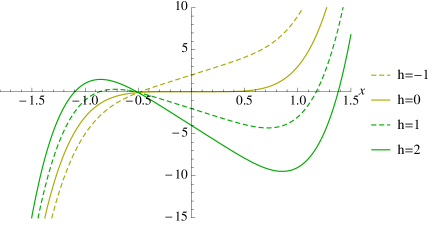
Figure 7: (Color online) Plots of the polynomial $3x^{5}-4hx-2h$ for several $h$. The roots of this polynomial determine the concentration points of $p_{\rm ave}(x)$ for $\epsilon\to 0$ in the model system considered below.

D.1 Euler-Lagrange equation (Instanton equation)

We consider the following finite time cumulant generating function:

$$G_{\tau,\epsilon}(h)=\frac{\epsilon}{\tau}\log\left\langle\mathrm{e}^{(\tau/\epsilon)h\Lambda(\tau)}\right\rangle_{\rm st},$$ (52)

where $\left\langle\ \right\rangle_{\rm st}$ means the average with respect to the path with a stationary initial condition. (Hereafter, we denote this initial distribution function by $P_{\rm st}(x)$.) The function $G_{\epsilon}(h)\equiv\lim_{\tau\rightarrow\infty}G_{\tau,\epsilon}(h)$ corresponds to $\tilde{G}(\tilde{h})$ in the main text. By taking $\epsilon\rightarrow 0$, we obtain the following variational principle:

$$\begin{split}&\lim_{\epsilon\rightarrow 0}G_{\tau,\epsilon}(h)\\ &=-\frac{1}{\tau}\min_{x_{0},x_{\tau}}\left[\min_{\underset{x(0)=x_{0},x(\tau)=x_{\tau}}{(x(t))_{t=0}^{\tau}}}\int_{0}^{\tau}L(\dot{x}(t),x(t))\mathrm{d}t+F_{\rm free}(x_{0})\right]\end{split}$$ (53)

with the Lagrangian $L(\dot{x},x)$ defined as

$$L(\dot{x},x)\equiv\frac{1}{4}\left(\dot{x}-F(x)\right)^{2}-h\lambda(x),$$ (54)

and also the free energy function $F_{\rm free}(x_{0})$ defined as

$$F_{\rm free}(x_{0})\equiv-\lim_{\epsilon\rightarrow 0}\epsilon\log P_{\rm st}(x_{0})=\frac{1}{4}x_{0}^{4}+\rm const.$$ (55)

Then, the corresponding Euler-Lagrange equation (Hamilton equation), which is obtained from minimising this action, is

$$\dot{x}=-x^{3}+2p$$ (56)

$$\dot{p}=3px^{2}-h(2x+1),$$ (57)

with the required initial and the final conditions as

$$p(0)=\frac{\partial F_{\rm free}(x)}{\partial x}\bigg{|}_{t=0}=x(0)^{3}$$ (58)

$$p(\tau)=0.$$ (59)

We analyse these equations numerically and analytically in InPreparation . The following results are based on that study.

D.2 Steady solutions

Here, we consider the steady solutions of these instantons, which is defined as the solution obtained from $\dot{x}_{\rm st}=\dot{p}_{\rm st}=0$ in (56) and (57). These conditions lead to

$$p_{\rm st}=\frac{1}{2}x_{\rm st}^{3}$$ (60)

and

$$3x_{\rm st}^{5}-4hx_{\rm st}-2h=0.$$ (61)

We plot the left-hand side of (61) as a function of $x$ in Fig. 7 for several fixed $h$. The figure shows that this equation has three solutions, when $h$ is larger than a certain value (larger than 0).

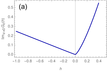
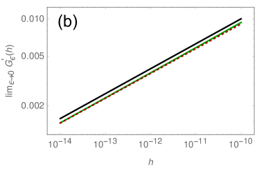
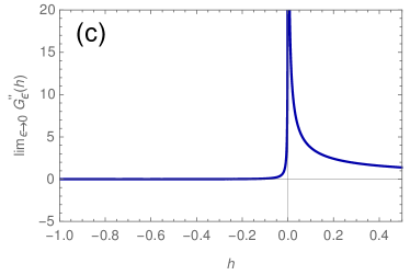
Figure 8: (Color online) (a) Generating function $\lim_{\epsilon\rightarrow 0}G_{\epsilon}(h)$. (b) The first derivatives, where the green (dark grey in the printed version) solid line represents $(d/dh)\lim_{\epsilon\rightarrow 0}G_{\epsilon}(h)$, the red dotted line represents $-(d/dh)\lim_{\epsilon\rightarrow 0}G_{\epsilon}(-h)$ and the black solid line represents a straight line $h^{1/5}$. From this panel, we find that the first derivative converges to 0 as a power law $\sim h^{1/5}$, (as can also be checked analytically). (c) The second derivative of $\lim_{\epsilon\rightarrow 0}G_{\epsilon}(h)$ with respect to $h$. These are calculated from (62-63). We can see that the second derivative shows a singularity at $h=0$, although the first derivative converges to 0. This represents a second-order dynamical phase transition.

D.3 Cumulant generating function

From the variational principle (53), even in the case where there are multiple instanton solutions, the cumulant generating function can be calculated. This is based on the observation that the instanton solution corresponding to the minimum is time-independent footnote:linearstabilityanalysis . More precisely, by combining this observation with the variational principle (53), we get

$$\lim_{\epsilon\rightarrow 0}G_{\epsilon}(h)=\max_{x_{\rm st}}G_{\rm st}(x_{\rm st}),$$ (62)

with

$$G_{\rm st}(x_{\rm st})\equiv-\frac{1}{4}x_{\rm st}^{6}+h\left(x_{\rm st}^{2}+x_{\rm st}\right).$$ (63)

We plot the $\epsilon\rightarrow 0$ result, $\lim_{\epsilon\rightarrow 0}G_{\epsilon}(h)$, in Fig. 8, from which we can see that the generating function has a kink at the origin, which is the sign of the dynamical phase transition in this system, appearing in the zero-temperature limit.Asymptotic analysis allows to find $G(h)\sim A_{\pm}|h|^{1/5}$ with $A_{\pm}$ depending on the sign of $h$, as illustrated on Fig. 8.

D.4 Analytical expressions of $p_{\rm end}(x)$ and $p_{\rm ave}(x)$ in $\epsilon\rightarrow 0$

Finally, we write the explicit analytical expressions of $p_{\rm end}(x)$ and $p_{\rm ave}(x)$ in the $\epsilon\rightarrow 0$ limit. We consider the biased (unnormalised) probability density $u^{h}$ introduced in the beginning of Section B.2. We also consider the same function but with fixed initial condition $u^{h}(x,\tau|x_{0},\tau)$. By using these function, we introduced two logarithmic functions defined as

$$W_{\rm F}(x,t)\equiv\epsilon\log u^{h}(x,t),$$ (64)

$$W_{\rm B}(x,t)\equiv\epsilon\log\int u^{h}(y,t|x,0)\mathrm{d}y.$$ (65)

From the generalised Feynman-Kac formula (38), we obtain the time evolution equation for them as

$$\begin{split}&\frac{\partial}{\partial t}W_{\rm F}(x,t)\\ &=-\epsilon\frac{\partial}{\partial x}F(x)-F(x)\frac{\partial}{\partial x}W_{\rm F}(x,t)\\ &\qquad+\epsilon\left(\frac{\partial}{\partial x}\right)^{2}W_{\rm F}(x,t)+\left(\frac{\partial}{\partial x}W_{\rm F}(x,t)\right)^{2}+h\lambda(x).\end{split}$$ (66)

and

$$\begin{split}&\frac{\partial}{\partial t}W_{\rm B}(x,t)\\ &=F(x)\frac{\partial}{\partial x}W_{\rm B}(x,t)+\epsilon\left(\frac{\partial}{\partial x}\right)^{2}W_{\rm B}(x,t)\\ &\qquad+\left(\frac{\partial}{\partial x}W_{\rm B}(x,t)\right)^{2}+h\lambda(x).\end{split}$$ (67)

These equations can be solved in $\epsilon=0$ with $t$ large limit. Indeed, by setting $W_{\rm F}(x,t)=tG(h)+W_{\rm F}(x)$ and $W_{\rm B}(x,\tau-t)=(\tau-t)G(h)+W_{\rm B}(x)$ with $G(h)\equiv\lim_{\epsilon\rightarrow 0}G_{\epsilon}(h)$ in these expressions, we obtain the equations to determine $W_{\rm F}(x)$ and $W_{\rm B}(x)$ as

$$\begin{split}&\frac{\partial W_{\rm F}(x)}{\partial x}=\frac{1}{2}\Bigg{[}F(x)\\ &+C_{h}(x)\sqrt{F(x)^{2}-4h\lambda(x)-\min_{y}\left[F(y)^{2}-4h\lambda(y)\right]}\Bigg{]},\end{split}$$ (68)

and

$$\begin{split}&\frac{\partial W_{\rm B}(x)}{\partial x}=\frac{1}{2}\Bigg{[}-F(x)\\ &+C_{h}(x)\sqrt{F(x)^{2}-4h\lambda(x)-\min_{y}\left[F(y)^{2}-4h\lambda(y)\right]}\Bigg{]}.\end{split}$$ (69)

with

$$C_{h}(x)=1\qquad(x<x_{\rm min}),$$ (70)

$$C_{h}(x)=-1\qquad(x>x_{\rm min}),$$ (71)

where

$$x_{\rm min}\equiv{\rm Argmin}_{x}\left[F(x)^{2}-4h\lambda(x)\right].$$ (72)

Equations (68) and (69) are the key result in this subsection. From them, we indeed get

$$\begin{split}&p_{\rm end}(x)\sim\exp\Bigg{[}(1/\epsilon)\int^{x}\frac{1}{2}\Big{[}F(y)\\ &+C_{h}(y)\sqrt{F(y)^{2}-4h\lambda(y)-\min_{z}\left[F(z)^{2}-4h\lambda(z)\right]}\Big{]}\mathrm{d}y\Bigg{]}\end{split}$$ (73)

and

$$\begin{split}&p_{\rm ave}(x)\sim\exp\Bigg{[}(1/\epsilon)\int^{x}C_{h}(y)\\ &\times\sqrt{F(y)^{2}-4h\lambda(y)-\min_{z}\left[F(z)^{2}-4h\lambda(z)\right]}\>\mathrm{d}y\Bigg{]}.\end{split}$$ (74)

Also from the same equations, we get the most probable $x$ in $p_{\rm end}(x)$ and $p_{\rm ave}(x)$ with $\epsilon\rightarrow 0$. We denote them by $x_{\rm end}$ and $x_{\rm ave}$, respectively. Then, from (73) and (74), we find that these values satisfy

$$x_{\rm ave}={\rm Argmax}_{x_{\rm st}}\ G_{\rm st}(x_{\rm st})$$ (75)

where $G_{\rm st}(h)$ is defined in (62), and

$$\frac{F(x_{\rm ave})^{2}}{4h}=\lambda(x_{\rm ave})-\lambda(x_{\rm end}).$$ (76)

Since $\frac{F(x_{\rm ave})^{2}}{4h}\neq 0$, $x_{\rm ave}$ and $x_{\rm end}$ are different from each other. In other words, $p_{\rm ave}$ and $p_{\rm end}$ concentrate on different values of their argument in the $\epsilon\rightarrow\infty$ limit, as announced in the main text.

For checking the validity of the obtained expressions, we numerically solve the equations (66) and (67) during a sufficiently large time interval $t$. We set $h=1$ (Fig. 9(a) and Fig. 9(c)) and $h=-1$ (Fig. 9(b) and Fig. 9(d)). The different colours represent the different values of $\epsilon$: yellow, blue, red lines correspond to $\epsilon=1,0.5,0.1$, respectively. In the same figure, we plot the analytical lines (68) and (69), with $C_{h}=1$ (for all $x$) (black solid line) and $C_{h}=-1$ (for all $x$) (black dashed line). We can see the convergence of the numerical lines (with decreasing $\epsilon$) towards the analytical lines (68) and (69), where $+$ sign is chosen for $x<x_{\rm min}$ and $-$ sign is chosen for $x>x_{\rm min}$.

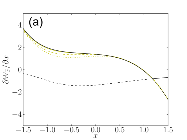
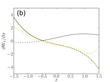
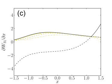
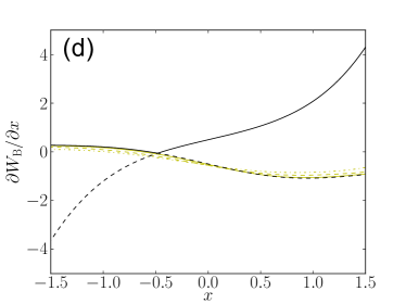
Figure 9: (Color online) The functions $\partial W_{\rm F}(x,t)/\partial x$ ((a) and (b)) and $\partial W_{\rm B}(x,t)/\partial x$ ((c) and (d)) obtained in the large $t$ limit by solving numerically (66) and (67) [yellow lines or light grey lines in the printed version]. We set $h=1$ ((a) and (c)) and $h=-1$ ((b) and (d)). The line types correspond different values of $\epsilon$: dash-dotted, dashed and solid lines correspond to $\epsilon=1,0.5,0.1$, respectively. To illustrate the determination of the $\pm$ sign of $C_{h}$ in the analytical results (68) and (69), we also plot on each subfigure those results with the choice of $C_{h}=1$ (for all $x$) as black solid lines and the choice of $C_{h}=-1$ (for all $x$) as black dashed lines. As the noise goes to zero, we observe the convergence of the functions $\partial W_{\rm F}(x,t)/\partial x$ and $\partial W_{\rm B}(x,t)/\partial x$ determined numerically at large $t$ towards the analytical line (68) and (69), where the $+$ sign in $\pm$ is taken for $x<x_{\rm min}$ and the $-$ sign is taken for $x>x_{\rm min}$.

References

- (1) S. Auer and D. Frenkel, Nature 409, 6823 (2001).
- (2) R. P. Sear, J. Phys.: Cond. Matt. 19, 033101(2007).
- (3) W. Ren, E. Vanden-Eijnden, P. Maragakis and W. E, J. Chem. Phys. 123, 134109 (2005).
- (4) M. Berhanu, et al., Europhys. Lett. 77, 59001 (2007).
- (5) F. Bouchet, and E. Simonnet, Phys. Rev. Lett. 102, 094504 (2009).
- (6) D. R. Easterling, G. A. Meehl, C. Parmesan, S. A. Changnon, T. R. Karl, L. O. Mearns, Science, 289, 2068 (2000).
- (7) C. Giardinà, J. Kurchan, and L. Peliti, Phys. Rev. Lett. 96, 120603 (2006).
- (8) J. Tailleur, and J. Kurchan, Nature Physics, 3, 203 (2007).
- (9) P. L. Ecuyer, V. Demers, and B. Tuffin, Proceedings of the 2006 Winter Simulation Conference, 137, (2006).
- (10) R. J. Allen, P. B. Warren, and P. R. ten Wolde, Phys. Rev. Lett. 94, 018104 (2005).
- (11) P. G. Bolhuis, D. Chandler, C. Dellago, and P. L. Geissler, Annu. Rev. Phys. Chem. 53, 291 (2002).
- (12) T. Nemoto and S.-i. Sasa, Phys. Rev. Lett. 112, 090602 (2014).
- (13) B. A. Berg and T. Neuhaus, Physics Letters B 267, 249 (1991).
- (14) F. Wang and D.P. Landau, Phys. Rev. Lett. 86, 2050 (2001).
- (15) L. Ortiz and L. Kaelbling, Proceedings of the Sixteenth Annual Conference on Uncertainty in Artificial Intelligence (UAI-2000), 446, (2000).
- (16) P. Dupuis and H. Wang, Ann. Appl. Prob. 15, 1 (2005).
- (17) O. Cappé, R. Douc, A. Guillin, J.-M. Marin and C. Robert, Stat. Comp. 18 587 (2008).
- (18) H. P. Chan and T. L. Lai, Ann. Appl. Prob. 21, 2315 (2011).
- (19) J. B. Anderson, J. Chem. Phys 63, 1499 (1975).
- (20) D. Aldous and U. Vazirani, in Proc. 35th IEEE Sympos. on Foundations of Computer Science (1994).
- (21) P. Grassberger, Comp. Phys. Comm. 147 64 (2002).
- (22) P. Del Moral, and J. Garnier, The Annals of Applied Probability, 15, 2496 (2005).
- (23) F. Cérou, A. Guyader, T. Lelièvre and D. Pommier, J. Chem. Phys. 134 054108 (2011).
- (24) J. Rolland, F. Bouchet and E. Simonnet, J. Stat. Phys. 162, 277 (2016).
- (25) H. Touchette, Phys. Rep. 478, 1, (2009).
- (26) A. Dembo and O. Zeitouni, Large deviations techniques and applications (Springer, New York, 1998).
- (27) L. O. Hedges, R. L. Jack, J. P. Garrahan and D. Chandler, Science 323 1309 (2009).
- (28) M. Picciani, M. Athènes,J. Kurchan and J. Tailleur, J. Chem. Phys. 135 034108 (2011).
- (29) J. K. Weber, R. L. Jack and V. S. Pande, J. Am. Chem. Soc. 135, 5501 (2013).
- (30) A. S. J. S. Mey, P. L. Geissler and J. P. Garrahan, Phys. Rev. E 89, 032109 (2014).
- (31) P. I. Hurtado, C. P. Espigares, J. J. del Pozo, P. L. Garrido, J. Stat. Phys. 154, 214 (2014).
- (32) B. Derrida, J. Stat. Mech. 2007, P07023 (2007).
- (33) P. I. Hurtado and P. L. Garrido, J. Stat. Mech. (2009) P02032.
- (34) All the results presented here can be generalised to models with interacting particles, by replacing and including interaction forces in . Markov jump processes are also workable.
- (35) C. W. Gardiner, Handbook of Stochastic Methods for Physics, Chemistry, and the Natural Sciences (Springer-Verlag, Berlin, 1983).
- (36) More precisely, when the Langevin equation (1) and the time-averaged quantity (4) are written in Stratonovich convention, one first transforms these equations to ones in Itō by using a transformation formula Gardiner , and then re-define and so that these transformed equations have the same forms as (1), (2), (3) and (4) (and can be analysed by the same method that is discussed throughout this paper).
- (37) It is also related to quantities in equilibrium thermodynamics. Indeed, when we set to be an external force, is the work done by the external system.
- (38) R. Chetrite and H. Touchette, Ann. Henri Poincare 16, 2005, (2015).
- (39) J. L. Lebowitz and H. Spohn, J. Stat. Phys. 95, 333 (1999).
- (40) V. Lecomte, C. Appert-Roland and F. van Wijland, J. Stat. Phys. 127, 51 (2007).
- (41) J. P. Garrahan, R. L. Jack, V. Lecomte, E. Pitard, K. van Duijvendijk and F. van Wijland, Phys. Rev. Lett. 98, 195702 (2007).
- (42) T. Bodineau and B. Derrida, Phys. Rev. E 72, 066110 (2005).
- (43) The matrix is assumed to be invertible but the generalization to non-invertible is direct.
- (44) H. Touchette, J. Stat. Phys. 159, 987 (2015).
- (45) V. Lecomte and J. Tailleur, J. Stat. Mech. (2007) P03004.
- (46) J. P. Garrahan, R. L. Jack, V. Lecomte, E. Pitard, K. van Duijvendijk, and F. van Wijland, J. Phys. A 42, 075007 (2009).
- (47) is also called the Kullback–Leibler divergence KBd . It is positive and measures the distance between the distributions and . It is zero if and only if those distributions are equal almost everywhere.
- (48) C. Kipnis and C. Landim, Scaling Limits of Interacting Particle Systems (Springer, New York, 1999).
- (49) W. Fleming and S. Mitter, Stochastics, 8, 63 (1982).
- (50) R. L. Jack and P. Sollich, Eur. Phys. J: Special Topics 224, 2351 (2015).
- (51) R. Chetrite and H. Touchette, J. Stat. Mech. 2015 P12001, (2015).
- (52) W. H. Fleming, Stochastic control and large deviations, in Future Tendencies in Computer Science, Control and Applied Mathematics, pages 291-300 (Springer, Berlin, 1992).
- (53) C. Hartmann and C. Schütte, J. Stat. Mech. (2012), P11004.
- (54) V. Y. Chernyak, M. Chertkov, J. Bierkens and H. J. Kappen, J. Phys. A 47, 022001 (2013).
- (55) R. M. L. Evans, Phys. Rev. Lett. 92, 150601 (2004).
- (56) R. L. Jack and P. Sollich, Prog. Theor. Phys. Suppl. 184, 304 (2010).
- (57) T. Nemoto and S.-i. Sasa, Phys. Rev. E 84, 061113 (2011).
- (58) C. Maes and K. Netocny, EPL 82, 30003 (2008).
- (59) T. Speck, A. Malins and C. P. Royall, Phys. Rev. Lett. 109, 195703 (2012).
- (60) R. L. Jack and P. Sollich, J. Phys. A 47, 015003 (2014).
- (61) The numerical calculations exploit an “annealing procedure” in which is reduced in steps of size , with the best estimate of from the each step being used as the first guess for in the subsequent step.
- (62) These integrands, which we denote by and , are proportional to each other when is small. Indeed, these satisfy . This is the reason why Fig. 6(a) and Fig. 6(b) show similarities.
- (63) Juan P. Garrahan and Igor Lesanovsky, Phys. Rev. Lett. 104, 160601 (2010).
- (64) James M. Hickey, Sam Genway, Igor Lesanovsky, and Juan P. Garrahan Phys. Rev. A 86, 063824 (2012).
- (65) J. Tailleur, V. Lecomte, AIP Conf. Proc, Vol 1091, pp. 212-219 (2009) MODELING AND SIMULATION OF NEW MATERIALS: Proceedings of Modeling and Simulation of New Materials: Tenth Granada Lectures.
- (66) In preparation by T. Nemoto and F. Bouchet.
- (67) We can prove this fact from a linear stability analysis. See InPreparation for the detail.
- (68) S. Kullback and R. A. Leibler, Annals of Mathematical Statistics 22 79 (1951).