State Feedback Stabilization of the Linearized Bilayer Saint-Venant Model

Abstract

We consider the problem of stabilizing the bilayer Saint-Venant model, which is a coupled system of two rightward and two leftward convecting transport partial differential equations (PDEs). In the stability proofs, we employ a Lyapunov function in which the parameters need to be successively determined. To the best of the authors’ knowledge, this is the first time this kind of Lyapunov function is employed, and this result is the first one on the stabilization of the linearized bilayer Saint-Venant model. Numerical simulations of the bilayer Saint-Venant problem are also provided to verify the result.

I Introduction

Population and economic growth are changing social values about the importance of water and the expansion of the energy sector will continue to drive growing demand for water resources. These trends are placing greater pressure on existing water allocations, heightening the importance of water management and conservation for the sustainability of irrigated agriculture. During the past decades, several efforts have been made by engineers and researchers towards the design of control methodologies for the real-time monitoring of irrigation canals. The global challenge motivating these studies is becoming increasingly obvious due to the less than desirable performance of both manually automatically controlled water management infrastructures.

In this paper, the $1$D two-layer Saint-Venant model that consists of the superposition of two immiscible fluids with different constant densities is presented. The derivation of the bilayer model can be found in [1] and [2]. The later one develops a stable well-balanced time-splitting scheme for a type of bilayer Saint-Venant model which satisfies a fully discrete entropy inequality. One can find some results on mathematical analysis of the related problem in [3] and [4]. To the best of the authors’ knowledge, the relevant control related problem for this application has not been investigated in the existing contributions.

PDE backstepping control approach has been successfully employed for the feedback stabilization of various classes of PDEs [5, 6]. In the present work, a general system, which consists of $m$ rightward and $n$ leftward transport PDEs with spatially varying coefficients, is exponentially stabilized by $m$ boundary input backstepping controllers. Our backstepping controller design idea can be referred to [7], in which the stabilization problem for the general coupled heterodirectional system of hyperbolic types with an arbritrary number of equations convecting in both directions is definitely solved. In our stability proofs, we employ a Lyapunov function in which the parameters need to be successively determined. Then, applying this general stabilization result to the 1D bilayer Saint-Venant problem, which consists of two rightward and two leftward convecting transport PDEs $(n=m=2)$, we achieve exponential stabilization with two boundary input controllers.

This paper is organized as follows. In Section II, we state the control problem. The 1D bilayer Saint-Venant model is first formulated based on its physical description, and then a linearized version around a steady state is presented. Section 3 is dedicated to the state feedback backstepping controller design of a more general system, for which and exponential stability is achieved for the closed-loop control system. This result could serve as a full theoretical result by itself, and it can be immediately utilized for the linearized bilayer Saint-Venant model. Numerical simulations are provided in Section 4. Finally in Section 5, a conclusion is presented and some perspectives are discussed.

II Problem Statement

II-A The 1D nonlinear bilayer Saint-Venant model

We consider the stabilization problem of a 1D two-layer Saint-Venant model, which governs the dynamic of two superposed immiscible layers of shallow water fluids.

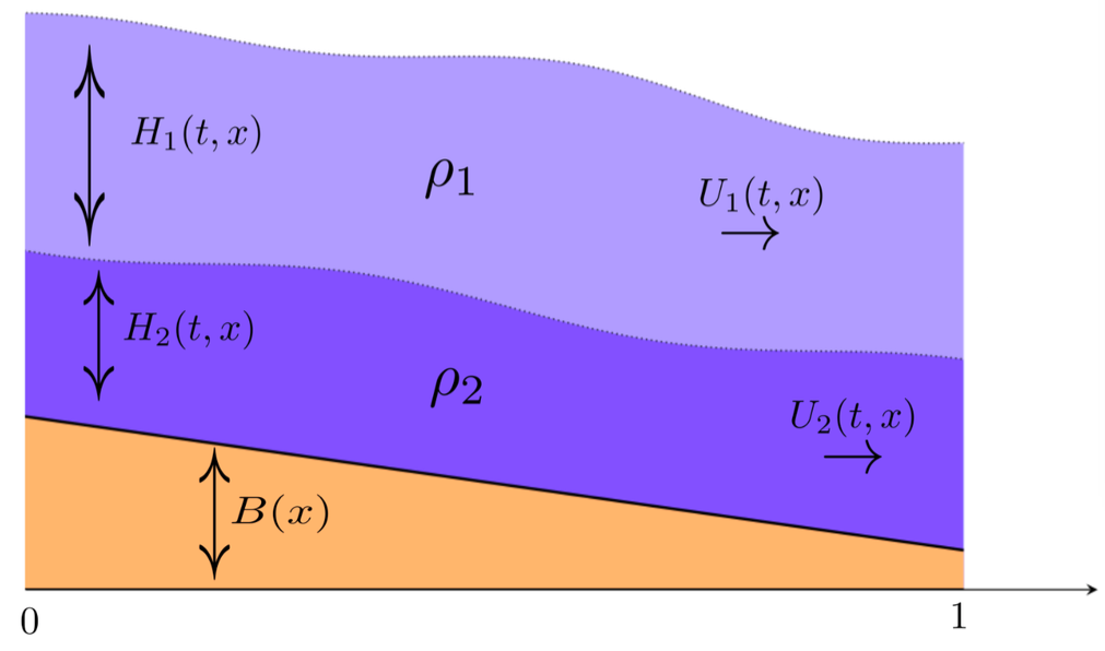
Figure 1: Two-layer shallow water flows with variable topography. $H_{\rm i}$ and $U_{\rm i}$ deote respectively the thickness of the layer $i$ and its velocity.

$$\left\{\begin{array}[]{ll}\frac{\partial H_{1}}{\partial t}+\frac{\partial(H_{1}U_{1})}{\partial x}=0,\\ \\ \frac{\partial U_{1}}{\partial t}+U_{1}\frac{\partial U_{1}}{\partial x}+g\frac{\partial H_{1}}{\partial x}+g\frac{\partial H_{2}}{\partial x}+g\frac{\partial B}{\partial x}=S_{1}^{f},\\ \\ \frac{\partial H_{2}}{\partial t}+\frac{\partial(H_{2}U_{2})}{\partial x}=0,\\ \\ \frac{\partial U_{2}}{\partial t}+U_{2}\frac{\partial U_{2}}{\partial x}+g\frac{\partial H_{2}}{\partial x}+g\frac{\rho_{1}}{\rho_{2}}\frac{\partial H_{1}}{\partial x}+g\frac{\partial B}{\partial x}=S_{2}^{f}.\end{array}\right.$$ (8)

In these equations, the index $1$ refers to the upper layer and the index $2$ to the lower one, as depicted in Figure 1. The unknown state variables $H_{i}$, $U_{i}$ and $B$ represent respectively the thickness of the $i$-th layer, the velocity and the height of the sediment layer. Each layer is assumed to have a constant density $\rho_{i}$, $i=1,2$ $(\rho_{1}<\rho_{2}).$ The system contains the source terms due to the bottom topography and the friction term. The quantities $S_{1}^{f}$ and $S_{2}^{f}$ stand as the friction between the two layers, and they are given by

$$S_{1}^{f}=-C_{f}|U_{1}-U_{2}|(U_{1}-U_{2})$$ (9)

and

$$S_{2}^{f}=rC_{f}|U_{1}-U_{2}|(U_{1}-U_{2}).$$ (10)

Define a vector $W=\begin{bmatrix}H_{1},&U_{1},&H_{2},&U_{2}\end{bmatrix}^{T}$, a ratio $r=\frac{\rho_{1}}{\rho_{2}}$ and a map

$$F(W)=\begin{bmatrix}H_{1}U_{1}\\ \frac{U^{2}_{1}}{2}+g(H_{1}+H_{2})\\ H_{2}U_{2}\\ \frac{U^{2}_{2}}{2}+g(H_{2}+rH_{1})\\ \end{bmatrix}$$ (11)

then we could recast equation (8) under the form of

$$\frac{\partial{W}}{\partial t}+\frac{\partial F(W)}{\partial x}=S(x,W),$$ (12)

where

$$S(x,W)\,=\,\begin{pmatrix}0&\ S_{1}^{f}-g\frac{\partial B}{\partial x}&\ 0&\ S_{2}^{f}-g\frac{\partial B}{\partial x}\end{pmatrix}^{T}.$$ (13)

By considering the Jacobian matrix $A$ from (12), we could rewrite the equation (12) into a quasilinear form as

$$\bm{\frac{\partial{W}}{\partial t}+A(W)\frac{\partial W}{\partial x}=S(x,W)},$$ (14)

where

$$A(W)=\begin{bmatrix}U_{1}&H_{1}&0&0\\ g&U_{1}&g&0\\ 0&0&U_{2}&H_{2}\\ rg&0&g&U_{2}\end{bmatrix}$$ (15)

Simple and exact analytical expression of the four eigenvalues of $A$ is not obvious. Complicate expression can be obtained tediously by applying the Cardano-Vieta method. For the case of $r\approx 1$ and $U_{1}\approx U_{2}$, a first order approximation of the eigenvalues is given in [8, 9].

In this work, we consider the case where $r\ll 1$, namely, when the bottom fluid is much thicker than the upper fluid. Moreover, recall that our problem is to consider the boundary controller design to stabilize (14).

II-B Linearization of the Saint-Venant model

We denote the steady-state associated to the system (14) by $W^{*}=(H_{1}^{*},U_{1}^{*},H_{2}^{*},U_{2}^{*})$, which satisfies the following equation of a compact form:

$$\bm{A(W^{*})\partial_{x}W^{*}=S(x,W^{*})}.$$ (16)

To obtain a constant steady-state, we work in the sequel with a flat bathymetry $(\partial_{x}B=0)$. A constant steady-state of the two-layer Saint-Venant equations can be characterized by:

$$\left\{\begin{array}[]{llll}H_{1}^{*}U_{1}^{*}=cste,\qquad H_{2}^{*}U_{2}^{*}=cste,\\ \frac{U_{1}^{*2}}{2}+g(H_{1}^{*}+H_{2}^{*})=-C_{f}|U_{1}^{*}-U_{2}^{*}|(U_{1}^{*}-U_{2}^{*}),\\ \frac{U_{2}^{*2}}{2}+g(H_{2}^{*}+rH_{1}^{*})=rC_{f}|U_{1}^{*}-U_{2}^{*}|(U_{1}^{*}-U_{2}^{*}).\end{array}\right.$$ (20)

In order to linearize the governing equations around the steady state, we define the deviation $(h_{1},u_{1},h_{2},u_{2})$ of the state $(H_{1},U_{1},H_{2},U_{2})$ with respect to the steady-state $(H_{1}^{*},U_{1}^{*},H_{2}^{*},U_{2}^{*})$ by:

$$\left\{\begin{array}[]{llll}h_{1}=H_{1}-H_{1}^{*},\qquad u_{1}=U_{1}-U_{1}^{*},\\ h_{2}=H_{2}-H_{2}^{*},\qquad u_{2}=U_{2}-U_{2}^{*}.\end{array}\right.$$ (23)

Then, the linearized version of (14) can be written in a matrix form as

$$\mathbf{\partial_{t}U+A^{*}\partial_{x}U=S_{l}(U)},$$ (24)

where

$$U=(h_{1},u_{1},h_{2},u_{2})^{T},\qquad A^{*}=A(W^{*}),$$

and

$$S_{l}(U)=[0\;-\alpha_{s}^{f}(u_{1}-u_{2})\;0\;r\alpha_{s}^{f}(u_{1}-u_{2})]^{T}$$

with

$$\alpha_{s}^{f}=2C_{f}|U_{1}^{*}-U_{2}^{*}|.$$

We consider a constant steady state here for the sake of readability and simplicity in the presentation of the linear model.

II-C Linearized Saint-Venant model in Riemann coordinates

We are to explore the system eigenstructure of the linear form (24) in this subsection. The characteristic equation derived from the matrix $A^{*}$ is

$$\Theta=rg^{2}H_{1}^{*}H_{2}^{*},$$ (25)

where

$$\Theta=\Big{(}(\lambda-U_{1}^{*})^{2}-gH_{1}^{*}\Big{)}\Big{(}(\lambda-U_{2}^{*})^{2}-gH_{2}^{*}\Big{)}.$$ (26)

For the case $r=0$, straightforward calculations lead to the following real eigenvalues for $A^{*}$:

$$\begin{array}[]{lll}\lambda_{1}=U_{1}^{*}-\sqrt{gH_{1}^{*}},\qquad\lambda_{2}=U_{1}^{*}+\sqrt{gH_{1}^{*}},\\ \lambda_{3}=U_{2}^{*}-\sqrt{gH_{2}^{*}},\qquad\lambda_{4}=U_{2}^{*}+\sqrt{gH_{2}^{*}}.\end{array}$$ (29)

We notice that the eigenvalues in this case are those corresponding to each layer separately. Following the results in [10], the eigenvalues for the system (14) in the case of $r\ll 1$ i.e $\rho_{1}\ll\rho_{2}$ approach to those given in (29). From (29), the internal and external characteristics travel at different speeds, and indeed, the lower layer characteristics moves much slower than the upper ones in the case of $r\ll 1$. Let us now recast the equation (24) into a diagonal form. For a given eigenvalue $\lambda_{k}$ $(k=1,2,3,4)$ of the matrix $A^{*}$, the associated right eigenvector is expressed by

$$V_{k}=\begin{bmatrix}1\\ \frac{\lambda_{k}-U_{1}^{*}}{H_{1}^{*}}\\ \frac{(\lambda_{k}-U_{1}^{*})^{2}-gH_{1}^{*}}{gH_{1}^{*}}\\ \frac{(\lambda_{k}-U_{2}^{*})((\lambda_{k}-U_{1}^{*})^{2}-gH_{1}^{*})}{gH_{1}^{*}H_{2}^{*}}\end{bmatrix}$$ (30)

Some computations lead to the associated left eigenvector $L_{k}$, which is given by:

$$L_{k}=-\frac{1}{(\lambda_{i}-\lambda_{k})(\lambda_{j}-\lambda_{k})(\lambda_{l}-\lambda_{k})}$$

$$\times\Big{[}l_{k,1}\quad l_{k,2}\quad l_{k,3}\quad l_{k,4}\Big{]}^{T}$$ (31)

for $i\neq j\neq l\neq k\in\{1,2,3,4\},$ where

$$l_{k,1} =U_{1}^{*3}-(trA^{*}-\lambda_{k})(U_{1}^{*2}+gH_{1}^{*})+f_{k}$$

$$+3gH_{1}^{*}-\frac{detA^{*}}{\lambda_{k}},$$ (32)

$$l_{k,2} =3H_{1}^{*}U_{1}^{*2}-2H_{1}^{*}U_{1}^{*}(trA^{*}-\lambda_{k})$$

$$+H_{1}^{*}(f_{k}+gH_{1}^{*}),$$ (33)

$$l_{k,3} =gH_{1}^{*}(7U_{1}^{*}-\lambda_{k}),\quad l_{k,4}=gH_{1}^{*}H_{2}^{*}.$$ (34)

The quantities $f_{k}$ are defined by:

$$f_{1}=(\lambda_{3}+\lambda_{2})\lambda_{4}+\lambda_{2}\lambda_{3},\,f_{2}=(\lambda_{3}+\lambda_{1})\lambda_{4}+\lambda_{1}\lambda_{3},$$ (35)

$$f_{3}=(\lambda_{2}+\lambda_{1})\lambda_{4}+\lambda_{1}\lambda_{2},\,f_{4}=(\lambda_{1}+\lambda_{2})\lambda_{3}+\lambda_{1}\lambda_{2}.$$ (36)

We are to express the linear version (24) of the governing equations in term of the characteristic coordinates or Riemann Invariants. Multiplying the equation (24) by the left eigenvectors $L_{k}$ (each for a given eigenvalue $\lambda_{k}$) of the matrix $A^{*}$, we get that the characteristic coordinates (Riemann Invariants) $\xi_{k}$ are:

$$\xi_{k}=L^{tr}_{k}U =-\frac{1}{(\lambda_{i}-\lambda_{k})(\lambda_{j}-\lambda_{k})(\lambda_{l}-\lambda_{k})},$$

$$\times\Big{[}l_{k,1}h_{1}+l_{k,2}u_{1}+l_{k,3}h_{2}+l_{k,4}u_{2}\Big{]}$$ (37)

for $i\neq j\neq l\neq k\in\{1,2,3,4\}$. Therefore, we can express the variables $h_{1}$, $u_{1}$, $h_{2}$ and $u_{2}$ in term of the Riemann coordinates:

$$\left\{\begin{array}[]{llll}h_{1}=\xi_{1}+\xi_{2}+\xi_{3}+\xi_{4},\\ u_{1}=\gamma_{1}\xi_{1}+\gamma_{2}\xi_{2}+\gamma_{3}\xi_{3}+\gamma_{4}\xi_{4},\\ h_{2}=\beta_{1}\xi_{1}+\beta_{2}\xi_{2}+\beta_{3}\xi_{3}+\beta_{4}\xi_{4},\\ u_{2}=\alpha_{1}\xi_{1}+\alpha_{2}\xi_{2}+\alpha_{3}\xi_{3}+\alpha_{4}\xi_{4},\end{array}\right.$$ (42)

where

$$\gamma_{k}=\frac{\lambda_{k}-1}{H_{1}^{*}},$$ (43)

$$\beta_{k}=\frac{1}{gH_{1}^{*}}\Big{(}U_{1}^{*2}+2(\lambda_{k}-1)U_{1}^{*}-\lambda_{k}^{2}+gH_{1}^{*}\Big{)},$$ (44)

and

$$\alpha_{k}= \frac{1}{gH_{1}^{*}H_{2}^{*}}\left((gH_{1}^{*}\beta_{k}-2\lambda_{k}^{2})U_{2}^{*}+3U_{1}^{*3}\right.$$

$$\left.+7(\lambda_{k}-1)U_{1}^{*2}+2(gH_{1}^{*}-2\lambda_{k}^{2})U_{1}^{*}\right.$$

$$\left.+\lambda_{k}^{2}(trA^{*}-\lambda_{k})+gH_{1}^{*}(\lambda_{k}+2)\right).$$ (45)

We introduce the following more compact notations:

$$\bm{\xi}=\begin{pmatrix}\xi_{1}&\xi_{2}&\xi_{3}&\xi_{4}\end{pmatrix}^{tr},\;\;$$ (46)

and

$${\bm{\Lambda}}=\text{diag}\{\lambda_{1},\lambda_{2},\lambda_{3},\lambda_{4}\}.$$ (47)

Using the characteristic coordinates, we recast the equation (24) into the following form:

$$\bm{\partial_{t}\xi+\Lambda\partial_{x}\xi=M\xi,}$$ (48)

where

$$M(W^{*})=\begin{pmatrix}0&\alpha_{s}^{f}&0&-r\alpha_{s}^{f}\end{pmatrix}^{tr}$$

$$~{}~{}~{}~{}~{}~{}~{}~{}~{}~{}~{}~{}~{}~{}\times\begin{pmatrix}\alpha_{1}-\gamma_{1}&\alpha_{2}-\gamma_{2}&\alpha_{3}-\gamma_{3}&\alpha_{4}-\gamma_{4}\end{pmatrix}.$$ (49)

We consider the case where both layers have a subcritical flow regime. Define the state vectors

$$u(t,x)=(\xi_{2},\xi_{4}),~{}v(t,x)=(\xi_{1},\xi_{3}),$$

and introduce the transport speed matrices

$${\bm{\Lambda}}^{\rm r}=\text{diag}\{\lambda_{2},\lambda_{4}\},~{}{-\bm{\Lambda}}^{\rm l}=\text{diag}\{\lambda_{1},\lambda_{3}\}.$$

Then, the system (48) can be rewritten as

$$\partial_{t}u(t,x)+\Lambda^{\rm r}\partial_{x}u(t,x) =S^{\rm r}u(t,x)$$

$$~{}~{}+S^{\rm l}v(t,x),$$ (50)

$$\partial_{t}v(t,x)-\Lambda^{\rm l}\partial_{x}v(t,x) =0,$$ (51)

where

$$S^{\rm r} =\begin{bmatrix}\alpha_{s}^{f}(\alpha_{1}-\gamma_{1})&\alpha_{s}^{f}(\alpha_{2}-\gamma_{2})\\ r\alpha_{s}^{f}(\gamma_{1}-\alpha_{1})&r\alpha_{s}^{f}(\gamma_{2}-\alpha_{2})\end{bmatrix},$$ (52)

$$S^{\rm l} =\begin{bmatrix}\alpha_{s}^{f}(\alpha_{3}-\gamma_{3})&\alpha_{s}^{f}(\alpha_{4}-\gamma_{4})\\ r\alpha_{s}^{f}(\gamma_{3}-\alpha_{3})&r\alpha_{s}^{f}(\gamma_{4}-\alpha_{4})\end{bmatrix}$$ (53)

To close the writing of the system (50)-(51), we enclose to it the following boundary and initial conditions:

$$u(t,0)=Q_{0}v(t,0)\text{ and }v(t,1)=R_{1}u(t,1)+\mathfrak{U}(t),$$ (54)

$$u(0,x)=u_{0}(x)\text{ and }v(0,x)=v_{0}(x),$$ (55)

where $Q_{0}$, $R_{1}$ $\in\mathcal{M}_{2,2}(\mathbb{R}),$ and $\mathfrak{U}(t)=(\mathfrak{u}_{1}(t),\mathfrak{u}_{2}(t))$ consists of the boundary controllers we need to design.

III controller design of a general system

In this section, we consider the backstepping controller design of a more general system, which could includes the Saint-Venant model as a special case. While solving our problem with the Saint-Venant model, it is also worth noting that the result derived in this section could be treated as a full theoretical result by itself.

III-A A more general control system

The more general system discussed in this section is

$$\partial_{t}u(t,x)+\Lambda^{\rm r}(x)\partial_{x}u(t,x)$$

$$~{}~{}~{}~{}~{}~{}~{}~{}~{}~{}~{}~{}=S^{\rm r}(x)u(t,x)+S^{\rm l}(x)v(t,x),$$ (56)

$$\partial_{t}v(t,x)-\Lambda^{\rm l}(x)\partial_{x}v(t,x)=S^{\rm o}(x)u(t,x),$$ (57)

where

$$u(x,t)=\begin{bmatrix}u_{1}(x,t),\,u_{2}(x,t),\,\dots,\,u_{n}(x,t)\\ \end{bmatrix},$$ (58)

$$v(x,t)=\begin{bmatrix}v_{1}(x,t),\,v_{2}(x,t),\,\dots,\,v_{m}(x,t)\\ \end{bmatrix}$$ (59)

are the systems states. The matrices

$${\bm{\Lambda^{\rm r}}}(x)=\text{diag}\begin{bmatrix}\lambda^{\rm r}_{1}(x)\,,\,\lambda^{\rm r}_{2}(x)\,,\,\cdots\,,\,\lambda^{\rm r}_{m-1}(x)\end{bmatrix},$$ (60)

$${\bm{\Lambda^{\rm l}}}(x)=\text{diag}\begin{bmatrix}\lambda^{\rm l}_{1}(x)\,,\,\lambda^{\rm l}_{2}(x)\,,\,\cdots\,,\,\lambda^{\rm l}_{m-1}(x)\end{bmatrix},$$ (61)

subject to the restriction

$$-\lambda^{\rm l}_{m}(x)<-\lambda^{\rm l}_{2}(x)\dots<-\lambda^{\rm l}_{1}(x)<0,$$ (62)

$$0<\lambda^{\rm r}_{1}(x)<\lambda^{\rm r}_{2}(x)<\dots<\lambda^{\rm r}_{n}(x),$$ (63)

and the in-domain parameters are given as

$$S^{\rm r}(x) =\{S^{\rm r}_{ij}(x)\}_{1\leq i\leq n,1\leq j\leq n},$$ (64)

$$S^{\rm l}(x) =\{S^{\rm l}_{ij}(x)\}_{1\leq i\leq n,1\leq j\leq m},$$ (65)

$$S^{\rm o}(x) =\{S^{\rm o}_{ij}(x)\}_{1\leq i\leq n,1\leq j\leq m}.$$ (66)

The system is also equipped with the following boundary and initial conditions:

$$u(t,0)=Q_{0}v(t,0)\text{ and }v(t,1)=R_{1}u(t,1)+\mathfrak{U}(t),$$ (67)

$$u(0,x)=u_{0}(x)\text{ and }v(0,x)=v_{0}(x),$$ (68)

where the boundary parameters $Q_{0}$, $R_{1}$ $\in\mathcal{M}_{m,n}(\mathbb{R})$ are given as

$$R_{1}=\{r_{ij}\}_{1\leq i\leq m,1\leq j\leq n}.$$ (69)

$$Q_{0} =\{q_{ij}(x)\}_{1\leq i\leq n,1\leq j\leq m,}$$ (70)

and the boundary controllers are given as

$$\mathfrak{U}(t)=\begin{bmatrix}\mathfrak{u}_{1}(t)&\mathfrak{u}_{2}(t)&\dots&\mathfrak{u}_{n}(t)\end{bmatrix}^{T}.$$ (71)

III-B Target system

We employ the PDE backstepping method. First, we construct a backstepping transformation to map the system (56)-(57) into a target system with desirable stability property, which follows from the one constructed in [7].

Consider the following target system

$$\partial_{t}\epsilon(t,x)+\Lambda^{\rm r}(x)\partial_{x}\epsilon(t,x)=S^{\rm r}(x)\epsilon(t,x)+S^{\rm l}(x)\beta(t,x)$$

$$+\int_{0}^{x}C^{\rm r}(x,\xi)\epsilon(\xi)d\xi+\int_{0}^{x}C^{\rm l}(x,\xi)\beta(\xi)d\xi$$ (72)

$$\partial_{t}\beta(t,x)-\Lambda^{\rm l}(x)\partial_{x}\beta(t,x)=\Delta(x)\beta(0,t)$$ (73)

with the following boundary conditions

$$\epsilon(t,0)=Q_{0}\beta(t,0)\text{ and }\beta(t,1)=0,$$ (74)

where

$$\Delta(x)=\begin{bmatrix}0&\cdots&\cdots&0\\ \delta_{2,1}(x)&\ddots&\ddots&\vdots\\ \vdots&\ddots&\ddots&\vdots\\ \delta_{m,1}(x)&\cdots&\delta_{m,m-1}(x)&0\end{bmatrix},$$ (75)

and $C^{\rm r},~{}C^{\rm l}$ are $L^{\infty}$ matrix functions defined on the triangular domain

$$\mathbb{T}=\Big{\{}(x,\xi)\in\mathbb{R}^{2}|\;0\leq\xi\leq x\leq 1\Big{\}}.$$

Here, $\Delta(x),~{}C^{\rm r},~{}C^{\rm l}$ are all to be determined by introducing a backstepping transformation later.

III-C Backstepping controller design

In order to map the system (56)-(57) into the desired target system (72)-(74), we consider the following backstepping transformation

$$\begin{pmatrix}\epsilon(t,x)\\ \beta(t,x)\end{pmatrix}=\begin{pmatrix}u(t,x)\\ v(t,x)\end{pmatrix}-\int_{0}^{x}\mathfrak{G}(x,\xi)\begin{pmatrix}u(t,\xi)\\ v(t,\xi)\end{pmatrix}d\xi,$$ (76)

where

$$\mathfrak{G}=\begin{pmatrix}0&0\\ G_{21}(x,\xi)&G_{22}(x,\xi)\end{pmatrix}.$$ (77)

Here the to-be-determined kernels $G_{21}$ and $G_{22}$ are defined on the domain $\mathbb{T}$, which need to satisfy the following system of equations:

$$\partial_{\xi}G_{21}(x,\xi){\bm{\Lambda^{\rm r}}}(\xi)-{\bm{\Lambda^{\rm l}}}(x)\partial_{x}G_{21}(x,\xi)$$

$$=\!\!-G_{21}(x,\xi)\frac{d{\bm{\Lambda^{\rm r}}}(\xi)}{d\xi}\!\!-\!\!G_{21}(x,\xi)S^{\rm r}(\xi)\!\!-\!\!G_{22}\!(x,\xi)S^{\rm o}\!(\xi)$$ (78)

$$\partial_{\xi}G_{22}(x,\xi){\bm{\Lambda^{\rm r}}}(\xi)+{\bm{\Lambda^{\rm l}}}(x)\partial_{x}G_{22}(x,\xi)$$

$$~{}~{}~{}~{}~{}=-G_{22}(x,\xi)\frac{d{\bm{\Lambda^{\rm r}}}(\xi)}{d\xi}+G_{21}(x,\xi)S^{\rm l}(\xi),$$ (79)

and the following boundary conditions:

$$G_{21}(x,x){\bm{\Lambda^{\rm r}}}(x)+{\bm{\Lambda^{\rm l}}}(x)G_{21}(x,x) =-S^{\rm o}(x),$$ (80)

$$G_{22}(x,x){\bm{\Lambda^{\rm l}}}(x)-{\bm{\Lambda^{\rm l}}}(x)G_{22}(x,x) =0,$$ (81)

$$G_{21}(x,0){\bm{\Lambda^{\rm r}}}(0)Q_{0}-G_{22}(x,0){\bm{\Lambda^{\rm l}}}(0) =-\Delta(x).$$ (82)

The existence, regularity and invertibility of the backstepping tranformation could be obtained similarly as [7], which is omitted here due to page limit consideration. Moreover, $\delta_{i,j}(x)$ for $i=\overline{2,~{}m}$ $j=\overline{1,~{}m-1}$ can be obtained from its inverse transformation. and the following equations are obtained for $C^{\rm r}(x,\xi)$, $C^{\rm l}(x,\xi)$:

$$C^{\rm r}(x,\xi) =S^{\rm l}(x)G_{21}(x,\xi)$$

$$~{}~{}~{}+\int_{\xi}^{x}C^{\rm l}(x,\eta)G_{21}(\xi,\eta)\,d\eta,$$ (83)

$$C^{\rm l}(x,\xi) =S^{\rm l}(x)G_{22}(x,\xi)$$

$$~{}~{}~{}~{}+\int_{\xi}^{x}C^{\rm l}(x,\eta)G_{22}(\xi,\eta)\,d\eta.$$ (84)

Hence, the control law $\mathfrak{U}(t)$ can be obtained by plugging the transformation (76) into (67). Readily, $\beta(t,1)=0$ implies that

$$\mathfrak{U}(t)=-R_{1}u(t,1)$$

$$~{}~{}~{}~{}~{}~{}~{}+\int_{0}^{1}\Big{[}G_{21}(1,\xi)u(t,\xi)+G_{22}(1,\xi)v(t,\xi)\Big{]}\,d\xi.\$$ (85)

III-D Stability of the Target system

Assume that there exist constants $M>0,\bar{q}>0$, such that

$$\|C^{r}(x,\xi)\|,\|C^{l}(x,\xi)\|,\|S^{\rm r}(x)\|,\|S^{\rm l}(x)\|\leq M,\$$

$$~{}~{}~{}~{}~{}~{}~{}~{}~{}~{}~{}~{}~{}~{}~{}~{}~{}~{}~{}~{}~{}~{}~{}~{}~{}~{}~{}~{}~{}~{}~{}~{}~{}~{}~{}~{}\forall x\in[0,1],\xi\in[0,x],$$ (86)

$$\|Q^{T}_{0}Q_{0}\|<\bar{q,}$$ (87)

where $\|\cdot\|$ denotes the $2$-norm, and denote

$$\min\{\lambda_{i}^{r}(x),\lambda_{i}^{l}(x);x\in[0,1],i=\overline{1,n}\}=\underline{\lambda},$$ (88)

$$\max\{\lambda_{i}^{r}(x),\lambda_{i}^{l}(x);x\in[0,1],i=\overline{1,n}\}=\overline{\lambda}.$$ (89)

We first prove exponential stability of the target system (72)-(74). The novelty, compared with other results in this area (i.e., [7]), lies in the newly proposed Lyapunov function. We employ a Lyapunov function that needs to be successively determined.

Lemma 1

For any given initial data $(\epsilon^{0},\ \beta^{0})^{T}$
=$(\epsilon(0,\cdot),\ \beta(0,\cdot))^{T}\,$ $\in\,\left(\mathcal{L}^{2}([0,1])\right)^{n+m}$ and under the assumption that $C^{\rm r},~{}C^{\rm l}\,\in\mathcal{C}(\mathbb{T})$, the equilibrium $(\epsilon,\ \ \beta)^{T}=(0,\ 0,\ 0,\ 0)^{T}$ of the target system (72)-(75) is exponentially stable in the $\mathcal{L}^{2}$-norm:

$$\|(\epsilon(t,\cdot),\beta(t,\cdot))\|^{2}_{\mathcal{L}^{2}}$$

$$~{}~{}~{}~{}~{}~{}~{}:=\int_{0}^{1}\epsilon^{T}(t,x)\epsilon(t,x)+\beta^{T}(t,x)\beta(t,x)dx.$$ (90)

PROOF:
We consider the following Lyapunov function:

$$V(t)=\frac{1}{2}\int_{0}^{1}e^{-\nu x}\epsilon^{T}(t,x)\bm{\Lambda^{\rm r}_{\rm inv}}(x)\epsilon(t,x)dx$$

$$~{}~{}~{}~{}~{}~{}+\frac{1}{2}\int_{0}^{1}(1+x)\beta^{T}(t,x)D\bm{\Lambda^{\rm l}_{\rm inv}}(x)\beta(t,x)dx,$$ (91)

where $D=\text{diag}\begin{bmatrix}d_{1}\,,\,d_{2}\,,\,\cdots\,,\,d_{m-1}\,,\,d_{m}\end{bmatrix}$, and

$${\bm{\Lambda}^{\rm r}_{\rm inv}(x)}=\text{diag}\left\{\frac{1}{\lambda^{\rm r}_{1}(x)},\dots,\frac{1}{\lambda^{\rm r}_{n}(x)}\right\},$$

$${\bm{\Lambda}^{\rm l}_{\rm inv}(x)}=\text{diag}\left\{\frac{1}{\lambda^{\rm l}_{1}(x)},\dots,\frac{1}{\lambda^{\rm l}_{m}(x)}\right\}$$

with $\left(\lambda^{\rm r}_{1}(x),\dots,\lambda^{\rm r}_{n}(x)\right)>0,~{}\left(\lambda^{\rm l}_{1}(x),\dots,\lambda^{\rm r}_{m}(x)\right)>0.$ The constants $\nu$ and $d_{1},\,d_{2}\,,\,\cdots\,,\,d_{m-1}$ are all positive parameters to be determined. Then, we have

$$C_{1}\!\|(\epsilon(t,\cdot),\beta(t,\cdot))\|^{2}_{\mathcal{L}^{2}}\!\!\leq V(t)\leq\!\!C_{2}\|(\epsilon(t,\cdot),\beta(t,\cdot))\|^{2}_{\mathcal{L}^{2}},$$ (92)

where the two positive constants are

$$C_{1}=\frac{1}{2\bar{\lambda}}\min\left\{e^{-\nu},~{}d_{i};i\,=\overline{1,m}\right\},$$ (93)

$$C_{2}=\frac{1}{2\underline{\lambda}}\max\left\{1,~{}2d_{i};i\,=\overline{1,m}\right\}.$$ (94)

This ensures that $V(t)$ is positive definite.

Differentiating (91) with respect to time, we get:

$$\dot{V}(t)=\int_{0}^{1}e^{-\nu x}\epsilon^{T}(t,x)\bm{\Lambda^{\rm r}_{\rm inv}}(x)\partial_{t}\epsilon(t,x)dx$$

$$~{}~{}~{}~{}~{}~{}~{}+\int_{0}^{1}(1+x)\beta^{T}(t,x)D\bm{\Lambda^{\rm l}_{\rm inv}}(x)\partial_{t}\beta(t,x)dx.$$ (95)

With the help of (72) and (73), we rewrite (95) as follows:

$$\dot{V}(t)= \int_{0}^{1}-e^{-\nu x}\epsilon^{T}(t,x)\partial_{x}\epsilon(t,x)dx$$

$$+\int_{0}^{1}e^{-\nu x}\epsilon^{T}(t,x)\bm{\Lambda^{\rm r}_{\rm inv}}(x)S^{\rm r}(x)\epsilon(t,x)dx$$

$$+\int_{0}^{1}e^{-\nu x}\epsilon^{T}(t,x)\bm{\Lambda^{\rm r}_{\rm inv}}(x)S^{\rm l}(x)\beta(t,x)dx$$

$$+\int_{0}^{1}e^{-\nu x}\epsilon^{T}(t,x)\left(\int_{0}^{x}\bm{\Lambda^{\rm r}_{\rm inv}}(x)C^{\rm r}(x,\xi)\epsilon(\xi)d\xi\right)dx$$

$$+\int_{0}^{1}e^{-\nu x}\epsilon^{T}(t,x)\left(\int_{0}^{x}\bm{\Lambda^{\rm r}_{\rm inv}}(x)C^{\rm l}(x,\xi)\beta(\xi)d\xi\right)dx$$

$$+\int_{0}^{1}(1+x)\beta^{T}(t,x)D\partial_{x}\beta(t,x)dx+I(t),$$ (96)

where

$$I(t)=\int_{0}^{1}(1+x)\beta^{T}(t,x)D\bm{\Lambda^{\rm l}_{\rm inv}}(x)\Delta(x)\beta(0,t)\,dx.$$ (97)

Since

$$I(t)\leq(m-1)\int_{0}^{1}\frac{(1+x)}{2}\beta^{T}(t,x)\beta(t,x)\,dx$$

$$+\beta_{1}(t,0)^{2}\int_{0}^{1}\frac{(1+x)}{2}\sum_{i=2}^{m}d_{i}^{2}\frac{1}{\lambda^{\rm l}_{i}(x)^{2}}\delta_{i,1}^{2}(x)dx$$

$$+\beta_{2}(t,0)^{2}\int_{0}^{1}\frac{(1+x)}{2}\sum_{i=3}^{m}d_{i}^{2}\frac{1}{\lambda^{\rm l}_{i}(x)^{2}}\delta_{i,2}^{2}(x)dx$$

$$+\cdots$$

$$+\beta_{m-2}(t,0)^{2}\int_{0}^{1}\frac{(1+x)}{2}\sum_{i=m-1}^{m}d_{i}^{2}\frac{1}{\lambda^{\rm l}_{i}(x)^{2}}\delta_{i,m-2}^{2}(x)dx$$

$$+\beta_{m-1}(t,0)^{2}\int_{0}^{1}\frac{(1+x)}{2}d_{m}^{2}\frac{1}{\lambda^{\rm l}_{m}(x)^{2}}\delta_{m,m-1}^{2}(x)dx,$$

then

$$\dot{V}(t)\leq J_{1}(t)+J_{2}(t),$$ (98)

where

$$J_{1}(t)$$

$$=\beta_{1}(t,0)^{2}$$

$$~{}~{}~{}\times\Bigg{\{}\frac{\bar{q}}{2}-\frac{1}{2}d_{1}+\int_{0}^{1}\frac{(1+x)}{2}\sum_{i=2}^{m}d_{i}^{2}\frac{1}{\lambda^{\rm l}_{i}(x)^{2}}\delta_{i,1}^{2}(x)dx\Bigg{\}}$$

$$+\beta_{2}(t,0)^{2}$$

$$\times\Bigg{\{}\frac{\bar{q}}{2}-\frac{1}{2}d_{2}+\int_{0}^{1}\frac{(1+x)}{2}\sum_{i=3}^{m}d_{i}^{2}\frac{1}{\lambda^{\rm l}_{i}(x)^{2}}\delta_{i,2}^{2}(x)dx\Bigg{\}}$$

$$+\cdots+\beta_{m-2}(t,0)^{2}\Bigg{\{}\frac{\bar{q}}{2}-\frac{1}{2}d_{m-2}$$

$$~{}~{}~{}~{}~{}~{}~{}~{}~{}~{}~{}~{}~{}~{}~{}+\int_{0}^{1}\frac{(1+x)}{2}\sum_{i=m-1}^{m}d_{i}^{2}\frac{1}{\lambda^{\rm l}_{i}(x)^{2}}\delta_{i,m-2}^{2}(x)dx\bigg{\}}$$

$$+\beta_{m-1}(t,0)^{2}\Bigg{\{}\frac{\bar{q}}{2}-\frac{1}{2}d_{m-1}$$

$$~{}~{}~{}~{}~{}~{}~{}~{}~{}~{}~{}~{}~{}~{}~{}~{}~{}~{}+\int_{0}^{1}\frac{(1+x)}{2}d_{m}^{2}\frac{1}{\lambda^{\rm l}_{m}(x)^{2}}\delta_{m,m-1}^{2}(x)dx\Bigg{\}}$$

$$+\beta^{2}_{m}(t,0)\bigg{\{}\frac{\bar{q}}{2}-\frac{1}{2}d_{m}\bigg{\}},$$ (99)

and

$$J_{2}(t)=-\frac{1}{2}f_{1}(\nu)\int_{0}^{1}e^{-\nu x}\epsilon^{T}(t,x)\epsilon(t,x)dx$$

$$~{}~{}~{}~{}~{}~{}~{}~{}~{}~{}~{}-\frac{1}{2}f_{2}(\nu)\int_{0}^{1}\beta^{T}(t,x)\beta(t,x)\,dx$$ (100)

with

$$f_{1}(\nu)=\nu-2\left(\frac{M}{\underline{\lambda}}\right)^{2}-\frac{M}{\underline{\lambda}}(5+\frac{1}{\nu}),$$ (101)

$$f_{2}(\nu)=\min\left\{d_{i};i\,=\overline{1,m}\right\}-2m+1-\frac{1}{\nu}.$$ (102)

First, choose the positive constants $d_{1},\,d_{2}\,,\,\cdots\,,\,d_{m-1}$ successively as follows:

$$d_{m}\geq\bar{q},$$

$$d_{m-1}\geq\bar{q}+\int_{0}^{1}(1+x)d_{m}^{2}\frac{1}{\lambda^{\rm l}_{m}(x)^{2}}\delta_{m,m-1}^{2}(x)dx,$$

$$d_{m-2}\geq\bar{q}+\int_{0}^{1}(1+x)\sum_{i=m-1}^{m}d_{i}^{2}\frac{1}{\lambda^{\rm l}_{i}(x)^{2}}\delta_{i,m-2}^{2}(x)dx,$$

$$~{}~{}~{}~{}~{}~{}~{}~{}~{}~{}~{}~{}~{}~{}~{}~{}~{}~{}~{}~{}~{}~{}\vdots$$

$$d_{2}\geq\bar{q}+\int_{0}^{1}(1+x)\sum_{i=3}^{m}d_{i}^{2}\frac{1}{\lambda^{\rm l}_{i}(x)^{2}}\delta_{i,2}^{2}(x)dx,$$

$$d_{1}\geq\bar{q}+\int_{0}^{1}(1+x)\sum_{i=2}^{m}d_{i}^{2}\frac{1}{\lambda^{\rm l}_{i}(x)^{2}}\delta_{i,1}^{2}(x)\,dx,$$ (103)

which guarantee that $J_{1}(t)$ is non-negative. Then, choose $\nu>0$ large enough to satisfy

$$f_{1}(\nu)>0,$$ (104)

$$f_{3}(\nu):=\bar{q}-2m+1-\frac{1}{\nu}>0.$$ (105)

from which we have

$$f_{2}(\nu)\geq f_{3}(\nu)>0.$$ (106)

Thus, it holds that

$$\dot{V}(t)\leq J_{2}(t)\leq-cV(t),$$ (107)

where

$$c=\underline{\lambda}\min\left\{f_{1}(\nu),~{}\frac{1}{\max\{d_{i};i\,=\overline{1,m}\}}f_{2}(\nu)\right\},$$ (108)

which gives

$$V(t)\leq V(0)e^{-ct}.$$ (109)

Finally, from (92), we derive

$$\|(\epsilon(t,\cdot),\beta(t,\cdot))\|_{\mathcal{L}^{2}} \leq\sqrt{\frac{C_{2}}{C_{1}}}\|(\epsilon^{0}(\cdot),\beta^{0}(\cdot))\|_{\mathcal{L}^{2}}e^{-ct},$$ (110)

where $C_{1},C_{2}$ are defined in (93), (94). This completes the proof.

III-E Stability of the closed-loop control system

With the exponential stability of the target system, and with existence, regularity and invertibility of the backstepping tranformation, we are now ready to derive the stability of the closed-loop control system.

Theorem 1

For any given initial data $(u^{0},\ v^{0})^{T}=\,$ $(u(0,\cdot),\ v(0,\cdot))^{T}\in\,\left(\mathcal{L}^{2}([0,1])\right)^{n+m}$ and under the assumption that $C^{\rm r},~{}C^{\rm l}\,\in\mathcal{C}(\mathbb{T})$, the equilibrium $(u,\ \ v)^{T}=(0,\ 0,\ 0,\ 0)^{T}$ of the closed-loop system (72)-(74) with the designed controller (85) is $\mathcal{L}^{2}$-exponentially stable.

The exponential stability result stated in Theorem 1 is immediatly applied to the linearized bilayer Saint-Venant model (8), in Riemanian coordinates, which consists of a coupled system of two rightward and two leftward convecting transport PDEs.

IV Simulation results

The goal of the following numerical simulations is to illustrate the efficiency of the designed $\mathfrak{U}(t)$, namely (85), to stabilize the linear system (48) around the zero equilibrium. As initial conditions, the following data are considered for the layer $1$ and $2$ through the physical variables

$$H_{2}(0,x)=2+0.5\exp\Big{(}-\frac{(x-0.5)^{2}}{0.003}\Big{)},\,H_{1}(0,x)=6-H_{1}(x)$$

and

$$U_{1}(0,x)=\frac{10}{H_{1}(0,x)}+3\sin(2\pi x),$$

$$U_{2}(0,x)=-\frac{10}{H_{2}(0,x)}-3\sin(2\pi x).$$

The initial data of the characteristic variables $\xi_{k}$, $(k=1,\,2,\,3,\,4)$ (for system (48)) are computed as function of the physical variables $H_{i}(0,x)$ and $U_{i}(0,x)$ for $i=1,\,2$, thanks to the relation (31). For the sake of simplicity, we consider the following uniform steady state:

$$H^{*}_{1}=3,\;U^{*}_{1}=1,\,H^{*}_{2}=1,\,U^{*}_{2}=0.95.$$

With this choice of steady state (set point), the characteristic speeds are given by:

$$\lambda_{1}=6.42,\,\lambda_{2}=4.08,\,\lambda_{3}=-4.42\text{ and }\lambda_{4}=-2.18.$$

Elsewhere, in the reported numerical experiments, the ratio $r$ between the densities is set to $0.01$ and the friction coefficient $C_{f}$ to $0.05$. We compute the solution up to time $T=10$. Regarding to the boundary conditions (68) the following matrix are considered

$$Q_{0}=\begin{bmatrix}-1.5&0.01\\ 0.01&1.5\\ \end{bmatrix},\quad R_{1}=\begin{bmatrix}0.5&0.1\\ 0.15&-0.5\\ \end{bmatrix}$$ (111)

Our implementation is based on an accurate finite volume method for the evolutionary equation (48). More precisely, we use a modified Roe’s scheme (see [11]). Since the computation of the designed control $\mathfrak{U}(t)$ requires the knowledge of the kernels $G_{21}$ and $G_{22}$, the kernel problems are solved numerically according to (III-C)-(82) using the finite element setup. As an illustration, the numerical solution of the second component of the kernel $G_{21}$ is given in Figure 2.

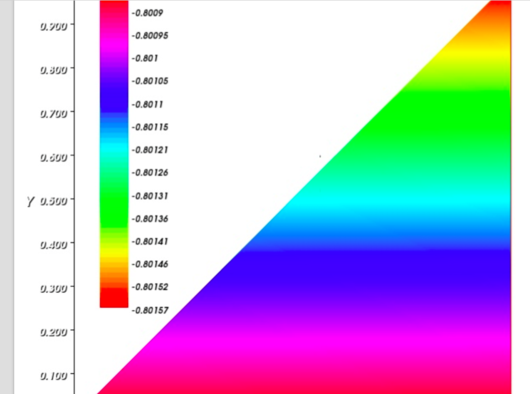
Figure 2: The kernel $G_{21}$.

Figure 3 depicts the evolution in time of the $\mathcal{L}^{2}$-norm of the characteristics. As expected from the theoretical part we observe clearly that the norm of all characteristics decreases in time and converges to zero. As a result, this shows that the system (48) converges to the zero equilibrium. Thereby the two-layer Saint-Venant model (8) also converges to ($H^{*}_{1}$, $U^{*}_{1}$, $H^{*}_{2}$, $U^{*}_{2}$).

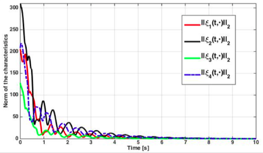
Figure 3: Evolution in time of the norm of the characteristic solutions.

In Figure 4 are depicted the behavior in time of each component of the input control $\mathfrak{U}(t)$. Clearly, despite the initial amplitude of $\mathfrak{u}_{2}(t)$, this latter one decreases in time and vanishes after $t\geq 4\,s$. Likewise $\mathfrak{u}_{2}(t)$, the first component of the control input $\mathfrak{u}_{1}(t)$ shows the same trend with its amplitude decreasing in time and tending to zero after $t\geq 7s$ as can be seen in Figure 4.

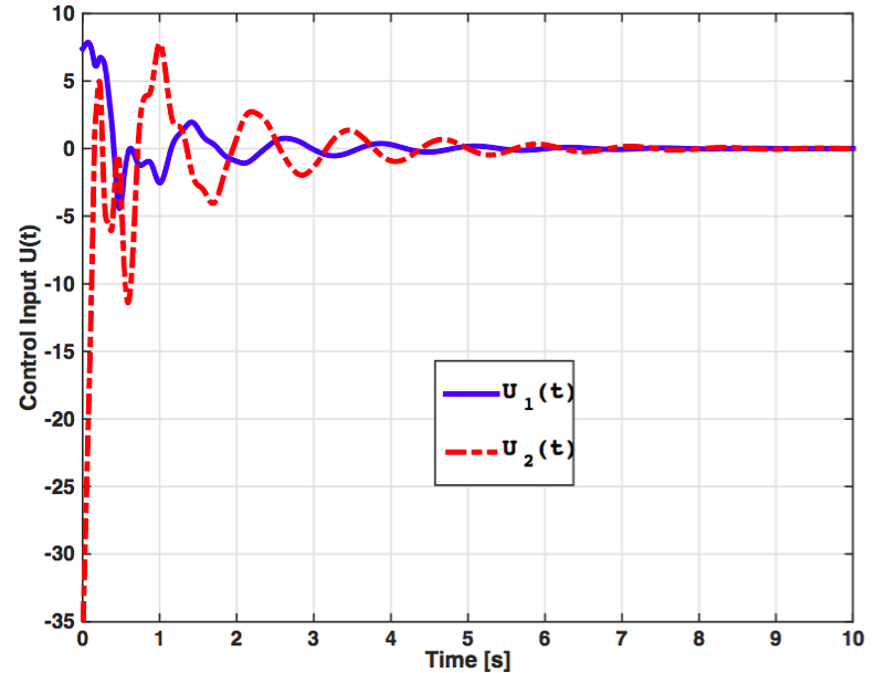
Figure 4: Evolution of the component of the control input $U(t)$.

As can be seen from these numerical simulations, the system (48) subject to the feedback control $\mathfrak{U}(t)$ is stabilized around the zero equilibrium as expected from the theoretical part.

V Conclusion and Future Works

In this paper, a general system with spatially varying coefficients, consisting of $m$ rightward and $n$ leftward convecting transport PDEs, is first exponentially stabilized by $m$ backstepping boundary controllers. Our controller design idea is similar as an existing result for this system with constant coefficients, and we employ a novel Lyapunov function in which the parameters need to be successively determined in the stability proofs. Then, this result is immediately applied to exponentially stabilize a 1D linearized bilayer Saint-Venant model, which is a coupled system of two rightward and two leftward convecting transport PDEs. One of our next steps is to consider the output feedback stabilizing of the general system, and then, as this paper, apply the result to the 1D bilayer Saint-Venant problem.

References

- [1] E. Audusse, M.-O. Bristeau, B. Perthame, and J. Sainte-Marie, “A multilayer saint-venant system with mass exchanges for shallow water flows. derivation and numerical validation,” ESAIM: Mathematical Modelling and Numerical Analysis, vol. 45, no. 1, pp. 169–200, 1 2011. [Online]. Available: http://eudml.org/doc/197421
- [2] F. Bouchut and d. L. T. Morales, “An entropy satisfying scheme for two-layer shallow water equations with uncoupled treatment,” ESAIM: Mathematical Modelling and Numerical Analysis, vol. 42, pp. 683–698, 7 2008.
- [3] G. Narbona-Reina and J. D. D. Zabsonre, “Existence of a global weak solution for a 2d viscous bi-layer shallow water model,” Nonlinear Analysis: Real World Applications, no. 10, pp. 2971–2984, 2009.
- [4] M. L. Munoz-Ruiz, F. J. Chatelon, and P. Orenga, “On a bi-layer shallow-water problem,” Nonlinear Analysis: Real World Applications, vol. 4, no. 1, pp. 139–171, 2003.
- [5] F. Di Meglio, R. Vazquez, and M. Krstic, “Stabilization of a system of coupled first-order hyperbolic linear PDEs with a single boundary input,” IEEE Transactions on Automatic Control, vol. 58, no. 12, pp. 3097–3111, 2013.
- [6] M. Krstic and A. Smyshlyaev, Boundary control of PDEs: A course on backstepping designs. Siam, 2008, vol. 16.
- [7] L. Hu, F. D. Meglio, R. Vazquez, and M. Krstic, “Control of homodirectional and general heterodirectional linear cou- pled hyperbolic pdes,” arXiv preprint arXiv:1504.07491, 2015.
- [8] E. F. Nieto, M. J. Castro-Diaz, and C. Parés, “On an intermediate field capturing riemann solver based on a parabolic viscosity matrix for the two-layer shallow water system,” Journal of Scientific Computing, vol. Volume 48, Issue 1-3, pp. 117–140, July 2011.
- [9] R. Abgrall and S. Karni, “Two-layer shallow water system: a relaxation approach,” SIAM J. Sci. Comput., vol. 31, No 3, pp. 1603–1627, 2009.
- [10] J. Schijf and J. Schonfeld, “Theoretical considerations on the motion of salt and fresh water,” Proc. of the Minn. Int. Hydraulics Conv. Joint meeting IAHR and Hyd. Div. ASCE., pp. 321–333, Sept. (1953).
- [11] R. J. LeVeque, Finite volume methods for hyperbolic problems, ser. Cambridge texts in applied mathematics. Cambridge, New York: Cambridge University Press, 2002.