Static solutions in Einstein-Chern-Simons gravity

Abstract

In this paper we study static solutions with more general symmetries than the spherical symmetry of the five-dimensional Einstein-Chern-Simons gravity. In this context, we study the coupling of the extra bosonic field $h^{a}$ with ordinary matter which is quantified by the introduction of an energy-momentum tensor field associated with $h^{a}$. It is found that exist (i) a negative tangential pressure zone around low-mass distributions ($\mu<\mu_{1}$) when the coupling constant $\alpha$ is greater than zero; (ii) a maximum in the tangential pressure, which can be observed in the outer region of a field distribution that satisfies $\mu<\mu_{2}$; (iii) solutions that behave like those obtained from models with negative cosmological constant. In such a situation, the field $h^{a}$ plays the role of a cosmological constant.

I Introduction

Five-dimensional Einstein-Chern-Simons gravity (EChS) is a gauge theory whose Lagrangian density is given by a 5-dimensional Chern-Simons form for the so called $\mathfrak{B}$ algebra salg1 . This algebra can be obtained from the AdS algebra and a particular semigroup $S$ by means of the $S$-expansion procedure introduced in Refs. salg2 ; salg3 . The field content induced by the $\mathfrak{B}$ algebra includes the vielbein $e^{a}$, the spin connection $\omega^{ab}$, and two extra bosonic fields $h^{a}$ and $k^{ab}.$ The EChS gravity has the interesting property that the five dimensional Chern-Simons Lagrangian for the $\mathfrak{B}$ algebra, given by salg1 :

$$L_{\mathrm{EChS}}=\alpha_{1}l^{2}\varepsilon_{abcde}R^{ab}R^{cd}e^{e}+\alpha_{3}\varepsilon_{abcde}\left(\frac{2}{3}R^{ab}e^{c}e^{d}e^{e}+2l^{2}k^{ab}R^{cd}T^{\text{ }e}+l^{2}R^{ab}R^{cd}h^{e}\right),$$ (1)

where $R^{ab}=\mathrm{d}\omega^{ab}+\omega_{\text{ }c}^{a}\omega^{cb}$ and $T^{a}=\mathrm{d}e^{a}+\omega_{\text{ }c}^{a}e^{c}$, leads to the standard General Relativity without cosmological constant in the limit where the coupling constant $l$ tends to zero while keeping the effective Newton’s constant fixed salg1 .

In Ref. salg4 was found a spherically symmetric solution for the Einstein-Chern-Simons field equations and then was shown that the standard five dimensional solution of the Einstein-Cartan field equations can be obtained, in a certain limit, from the spherically symmetric solution of EChS field equations. The conditions under which these equations admit black hole type solutions were also found.

The purpose of this work is to find static solutions with more general symmetries than the spherical symmetry. These solutions are represented by three-dimensional maximally symmetric spaces: open, flat and closed.

The functional derivative of the matter Lagrangian with respect to the field $\ h^{a}$ is considered as another source of gravitational field, so that it can be interpreted as a second energy-momentum tensor: the energy-momentum tensor for field $\ h^{a}$. This tensor is modeled as an anisotropic fluid, the energy density, the radial pressure and shear pressures are characterized. The results lead to identify the field $h^{a}$ with the presence of a cosmological constant. The spherically symmetric solutions of Ref. salg4 can be recovered from the general static solutions.

The article is organized as follows: In section II we briefly review the Einstein-Chern-Simons field equations together with their spherically symmetric solution, which lead, in certain limit, to the standard five-dimensional solution of the Einstein-Cartan field equations. In section III we obtain general static solutions for  the Einstein-Chern-Simons field equations. The obtaining of the energy momentum tensor for the field $h^{a},$ together with the conditions that must be satisfied by the energy density and radial and tangential pressures, also will be considered in section III. In section IV we recover the spherically symmetric black hole solution found in Ref. salg4 from the general static solutions and will study the energy density and radial and tangential pressures for a naked singularity and black hole solutions. Finally, concluding remarks are presented in section V.

II Spherically symmetric solution of EChS field equations

In this section we briefly review the Einstein-Chern-Simons field equations together with their spherically symmetric solution. We consider the field equations for the Lagrangian

$$L=L_{\mathrm{EChS}}+L_{\mathrm{M}},$$ (2)

where $L_{\mathrm{EChS}}$ is the Einstein-Chern-Simons gravity Lagrangian given in (1) and $L_{\mathrm{M}}$ is the corresponding matter Lagrangian.

In the presence of matter described by the langragian $L_{\mathrm{M}}=L_{\mathrm{M}}(e^{a},h^{a},\omega^{ab}),$ the field equations obtained from the action (2) when $T^{a}=0$ and $k^{ab}=0$ are given by salg4 :

$$\mathrm{d}e^{a}+\omega_{\text{ }b}^{a}e^{b}=0,$$ (3)

$$\varepsilon_{abcde}R^{cd}\mathrm{D}_{\omega}h^{e}=0,$$ (4)

$$\alpha_{3}l^{2}\star\left(\varepsilon_{abcde}R^{bc}R^{de}\right)=-\star\left(\frac{\delta L_{\mathrm{M}}}{\delta h^{a}}\right),$$ (5)

$$\star\left(\varepsilon_{abcde}R^{bc}e^{d}e^{e}\right)+\frac{1}{2\alpha}l^{2}\star\left(\varepsilon_{abcde}R^{bc}R^{de}\right)=\kappa_{\mathrm{EH}}\hat{T}_{a},$$ (6)

where $\mathrm{D}_{\omega}$ denotes the exterior covariant derivative respect to the spin connection $\omega$, “$\star$” is the Hodge star operator, $\alpha:=\alpha_{3}/\alpha_{1}$, $\kappa_{\mathrm{EH}}$ is the coupling constant in five-dimensional Einstein-Hilbert gravity,

$$\hat{T}_{a}=\hat{T}_{ab}e^{b}=-\star\left(\frac{\delta L_{\mathrm{M}}}{\delta e^{a}}\right)$$

is the energy-momentum 1-form, with $\hat{T}_{ab}$ the usual energy-momentum tensor of matter fields, and where we have considered, for simplicity, $\delta L_{M}/\delta\omega^{ab}=0.$

Since equation (6) is the generalization of the Einstein field equations, it is useful to rewrite it in the form

$$\star\left(\varepsilon_{abcde}R^{bc}e^{d}e^{e}\right)=\kappa_{\mathrm{EH}}\hat{T}_{a}+\frac{1}{2\alpha\alpha_{3}}\star\left(\frac{\delta L_{\mathrm{M}}}{\delta h^{a}}\right)$$ (7)

where we have used the equation (5). This result leads to the definition of the 1-form energy-momentun associated with the field $h^{a}$

$$\hat{T}_{a}^{(h)}=\hat{T}_{ab}^{(h)}e^{b}=\frac{1}{2\alpha\alpha_{3}}\star\left(\frac{\delta L_{\mathrm{M}}}{\delta h^{a}}\right).$$ (8)

This allows to rewrite the field equations (5) and (6) as

$$-\mathrm{sgn}(\alpha)\frac{1}{2}l^{2}\star\left(\varepsilon_{abcde}R^{bc}R^{de}\right)=\kappa_{\mathrm{EH}}\hat{T}_{a}^{(h)},$$ (9)

$$\star\left(\varepsilon_{abcde}R^{bc}e^{d}e^{e}\right)+\mathrm{sgn}(\alpha)\frac{1}{2}l^{2}\star\left(\varepsilon_{abcde}R^{bc}R^{de}\right)=\kappa_{\mathrm{EH}}\hat{T}_{a},$$ (10)

where the absolute value of the constant $\alpha$ has been absorbed by redefining the parameter $l$

$$l\rightarrow l^{\prime}=\frac{1}{\sqrt{\left|\alpha\right|}}=\sqrt{\left|\frac{\alpha_{1}}{\alpha_{3}}\right|}.$$

II.1 Static and spherically symmetric solution

In this subsection we briefly review the spherically symmetric solution of the EChS field equations, which lead, in certain limit, to the standard five-dimensional solution of the Einstein-Cartan field equations.

In five dimensions the static and spherically symmetric metric is given by

$$\mathrm{d}s^{2}=-f^{2}(r)\mathrm{d}t^{2}+\frac{\mathrm{d}r^{2}}{g^{2}(r)}+r^{2}\mathrm{d}\Omega_{3}^{2}=\eta_{ab}e^{a}e^{b},$$

where $\mathrm{d}\Omega_{3}^{2}=\mathrm{d}\theta_{1}^{2}+\sin^{2}\theta_{1}\mathrm{d}\theta_{2}^{2}+\sin^{2}\theta_{1}\sin^{2}\theta_{2}\mathrm{d}\theta_{3}^{2}$ is the line element of 3-sphere $S^{3}$.

Introducing an orthonormal basis

$$e^{T}=f(r)\,\mathrm{d}t,\ e^{R}=\frac{\mathrm{d}r}{g^{2}(r)},\ e^{1}=r\,\mathrm{d}\theta_{1},$$

$$e^{2}=r\sin\theta_{1}\,\mathrm{d}\theta_{2},\ e^{3}=r\sin\theta_{1}\sin\theta_{2}\,\mathrm{d}\theta_{3}$$ (11)

and replacing into equation (10) in vacuum ($\hat{T}_{TT}=\hat{T}_{RR}=\hat{T}_{ii}=0$), we obtain the EChS field equations for a spherically symmetric metric equivalent to eqs. (blue26 - blue28) from Ref. salg4 .

II.1.1 Exterior solution

Following the usual procedure, we find the following solution salg4 :

$$f^{2}(r)=g^{2}(r)=1+\text{sgn}(\alpha)\left(\frac{r^{2}}{l^{2}}-\beta\sqrt{\frac{r^{4}}{l^{4}}+\text{sgn}(\alpha)\frac{\kappa_{\mathrm{EH}}}{6\pi^{2}l^{2}}M}\right),$$ (12)

where $M$ is a constant of integration and $\beta=\pm 1$ shows the degeneration due to the quadratic character of the field equations. From (12) it is straightforward to see that when $l\rightarrow 0$, it is necessary to consider $\beta=1$ to obtain the standard solution of the Einstein-Cartan field equation, which allows to identify the constant $M$, with the mass of distribution.

III General Static Solutions with General Symmetries

In Ref. salg4 were studied static exterior solutions with spherically symmetry for the Einstein-Chern-Simons field equations in vacuum. In this reference were found the conditions under which the field equations admit black holes type solutions and were studied the maximal extension and conformal compactification of such solutions.

In this section we will show that the equations of Einstein-Chern-Simons allow more general solutions that found for the case of spherical symmetry. The spherical symmetry condition will be relaxed so as to allow studying solutions in the case that the space-time is foliated by maximally symmetric spaces more general than the 3-sphere. It will also be shown that, for certain values of the free parameters, these solutions lead to the solutions found in Ref. salg4 .

III.1 Solutions to the EChS field equations

Following Refs. Oliv01 ; Oliv02 , we consider a static metric of the form

$$\mathrm{d}s^{2}=-f^{2}(r)\,\mathrm{d}t^{2}+\frac{\mathrm{d}r^{2}}{g^{2}(r)}+r^{2}\mathrm{d}\Sigma_{3}^{2}.$$ (13)

where $\mathrm{d}\Sigma_{3}^{2}$ is the line element of a three-dimensional Einstein manifold $\Sigma_{3}$, which is known as the base manifold 7 .

Introducing an ortonormal basis, we have

$$e^{T}=f(r)\ \mathrm{d}t,\quad e^{R}=\frac{\mathrm{d}r}{g(r)},\quad e^{m}=r\tilde{e}^{m},$$

where $\tilde{e}^{m}$, with $m=\{1,2,3\}$, is the dreibein of the base manifold $\Sigma_{3}$.

From eq. (3), it is possible to obtain the spin connection in terms of the vielbein. From Cartan’s second structural equation $R^{ab}=\mathrm{d}\omega^{ab}+\omega_{\text{ }c}^{a}\omega^{cb}$ we can calculate the curvature matrix. The nonzero components are

$$R^{TR} =-\left(\frac{f^{\prime\prime}}{f}g^{2}+\frac{f^{\prime}}{f}g^{\prime}g\right)e^{T}e^{R},\ R^{Tm}=-\frac{f^{\prime}}{f}g^{2}e^{T}\tilde{e}^{m},$$

$$R^{Rm} =-g^{\prime}g\,e^{R}\tilde{e}^{m},\ R^{mn}=\tilde{R}^{mn}-g^{2}\tilde{e}^{m}\tilde{e}^{n},$$ (14)

where $\tilde{R}^{mn}=\mathrm{d}\tilde{\omega}^{mn}+\tilde{\omega}_{\text{ \ }p}^{m}\tilde{\omega}^{pn}$ are the components of the curvature of the base manifold. To define the curvature of the base manifold is necessary to define the spin connection $\tilde{\omega}^{mn}$ of the base manifold. This connection can be determined in terms of the dreibein $\tilde{e}^{m}$ using the property that the total covariant derivative of the vielbein vanishes identically, and the condition of zero torsion $\tilde{T}^{m}=0$.

Replacing the components of the curvature (14) in the field equations (10), for the case where $\hat{T}_{a}=0$ (vacuum), we obtain three equations

$$B_{u}(r)\tilde{R}(\tilde{x})+6A_{u}(r)=0,\quad u=\{0,1,2\},$$ (15)

where $\tilde{R}(\tilde{x})$ is the Ricci scalar of the base manifold and the functions $A_{u}(r)$ and $B_{u}(r)$ are given by

$$A_{0}(r) =-2r\left(g^{2}r^{2}\right)^{\prime}+\text{sgn}(\alpha)\,l^{2}r\left(g^{4}\right)^{\prime},$$ (16)

$$B_{0}(r) =2r\left(2r-\text{sgn}(\alpha)\,l^{2}\left(g^{2}\right)^{\prime}\right),$$ (17)

$$A_{1}(r) =2r\left(-2rg^{2}-3\,\text{sgn}(\alpha)\,l^{2}r^{2}g^{2}\frac{f^{\prime}}{f}+2\,\text{sgn}(\alpha)\,l^{2}g^{4}\frac{f^{\prime}}{f}\right),$$ (18)

$$B_{1}(r) =2r\left(2r-2\,\text{sgn}(\alpha)\,l^{2}g^{2}\frac{f^{\prime}}{f}\right),$$ (19)

$$A_{2}(r) =-2r^{2}\left(2\left(g^{2}r^{2}\right)^{\prime}+4rg^{2}\frac{f^{\prime}}{f}+r^{2}\left(g^{2}\right)^{\prime}\frac{f^{\prime}}{f}+2r^{2}g^{2}\frac{f^{\prime\prime}}{f}\right)$$

$$\qquad+\text{sgn}(\alpha)\,l^{2}r^{2}\left(3\left(g^{4}\right)^{\prime}\frac{f^{\prime}}{f}+4g^{4}\frac{f^{\prime\prime}}{f}\right)\left(g^{4}\right)^{\prime},$$ (20)

$$B_{2}(r) =2r\left\{2-\text{sgn}(\alpha)\,l^{2}\left(\left(g^{2}\right)^{\prime}\frac{f^{\prime}}{f}+2g^{2}\frac{f^{\prime\prime}}{f}\right)\right\}.$$ (21)

The equation (15) with $u=0$ can be rewritten as

$$-\frac{A_{0}(r)}{B_{0}(r)}=\frac{\tilde{R}(\tilde{x})}{6}.$$

Since the left side depends only on $r$ and the right side depends only on $\tilde{x}$, we have that both sides must be equal to a constant $\gamma$, so that

$$\tilde{R}(\tilde{x})=6\gamma.$$ (22)

An Einstein manifold $\Sigma_{n}$ is a Riemannian or pseudo Riemannian manifold whose Ricci tensor is proportional to the metric

$$\tilde{R}_{\mu\nu}=kg_{\mu\nu}.$$ (23)

The contraction of eq. (23) with the inverse metric $g^{\mu\nu}$ reveals that the constant of proportionality $k$ is related to the scalar curvature $\tilde{R}$ by

$$\tilde{R}=nk,$$ (24)

where $n$ is the dimension of $\Sigma_{n}$.

Introducing (23) and (24) into the so called contracted Bianchi identities,

$$\tilde{\partial}^{\beta}\left(\tilde{R}_{\alpha\beta}-\frac{1}{2}g_{\alpha\beta}\tilde{R}\right)=0,$$

we find

$$\left(n-2\right)\tilde{\partial}_{\beta}k=0.$$

This means that if $\Sigma_{n}$ is a Riemannian manifoldof dimension $n>2$ with metric $g_{\alpha\beta}$, then $k$ must be a constant.

On the other hand, in a $n$-dimensional space, the Riemann tensor can be decomposed into its irreducible components

$$\tilde{R}_{\mu\nu\rho\sigma} = \tilde{C}_{\mu\nu\rho\sigma}+\frac{1}{n-2}\left(g_{\mu\rho}\tilde{R}_{\nu\sigma}-g_{\mu\sigma}\tilde{R}_{\nu\rho}-g_{\nu\rho}\tilde{R}_{\mu\sigma}+g_{\nu\sigma}\tilde{R}_{\mu\rho}\right)$$ (25)

$$+\frac{1}{\left(n-1\right)\left(n-2\right)}\left(g_{\mu\sigma}g_{\nu\rho}-g_{\mu\rho}g_{\nu\sigma}\right)\tilde{R},$$

where $\tilde{C}_{\mu\nu\rho\sigma}$ is the Weyl conformal tensor, $\tilde{R}_{\alpha\beta}$ is the Ricci tensor and $\tilde{R}$ is the Ricci scalar curvature.

Introducing (23), (24) into (25) we have

$$\tilde{R}_{\mu\nu\rho\sigma}=\tilde{C}_{\mu\nu\rho\sigma}+\kappa\left(g_{\mu\rho}g_{\nu\sigma}-g_{\mu\sigma}g_{\nu\rho}\right),$$ (26)

where $\kappa=k/(n-1)$.

From (26) we can see that when $\tilde{C}_{\mu\nu\rho\sigma}=0$, the Einstein manifold $\Sigma_{n}$ is a Riemannian manifold with constant curvature $\kappa$.

Since the Weyl tensor is identically zero when $n=3$, we have that, if $n=3$, there is no distinction between Einstein manifolds and constant curvarture manifolds. However, for $n>3$, constant curvature manifolds are special cases of Einstein manifolds. This means that our $\Sigma_{3}(\tilde{x})$ manifold is a Riemannian manifold of constant curvature $\kappa=6\gamma$.

The solution of $A_{0}(r)/B_{0}(r)=-\gamma$ leads to

$$g^{2}(r)=\gamma+\text{sgn}(\alpha)\left(\frac{r^{2}}{l^{2}}-\beta\sqrt{\frac{r^{4}}{l^{4}}+\text{sgn}(\alpha)\frac{\mu}{l^{4}}}\right),$$

where $\mu$ is a constant of integration and $\beta=\pm 1$. The equations (15) with $u=0$ and $u=1$ lead to $f^{2}(r)=g^{2}(r)$, while $u=2$ tells us that

$$\tilde{R}=6\lambda,$$

where the constant of integration $\lambda$ must be equal to $\gamma$, so that is consistent with eq. (22).

In short, if the line element is given by (13), then the functions $f(r)$ and $g(r)$ are given by

$$f^{2}(r)=g^{2}(r)=\gamma+\text{sgn}(\alpha)\frac{r^{2}}{l^{2}}-\text{sgn}(\alpha)\,\beta\sqrt{\frac{r^{4}}{l^{4}}+\text{sgn}(\alpha)\frac{\mu}{l^{4}}}$$ (27)

where $\beta=\pm 1$ shows the degeneration due to the quadratic character of the field equations, $\mu$ is a constant of integration related to the mass of the system and $\gamma$ is another integration constant related to the scalar curvature of the base manifold ($\tilde{R}=6\gamma$): $\gamma=0$ if it is flat, $\gamma=-1$ if it is hyperbolic (negative curvature) or $\gamma=1$ if it is spherical (positive curvature).

III.2 A solution for equation (4)

Since the explicit form of the $h^{a}$ field is important in an eventual construction of the matter lagrangian $L_{M}$, we are interested in to solve the field equation (4) for the $h^{a}$ field.

$$\varepsilon_{abcde}R^{cd}\mathrm{D}_{\omega}h^{e}=0.$$ (28)

Expanding the $h^{a}=h_{\text{ }\mu}^{a}dx^{\mu}$ field in their holonomic index, we have

$$h_{a}=h_{\mu\nu}e_{a}^{\mu}\,\mathrm{d}x^{\nu}.$$

For the space-time with a three-dimensional manifold maximally symmetrical $\Sigma_{3}$, we will assume that the field $h_{\mu\nu}$ must satisfy the Killing equation $\mathcal{L}_{\xi}h_{\mu\nu}=0$ for $\xi_{0}=\partial_{t}$ (stationary) and the six generators of the $\Sigma_{3}$, i.e., we are assuming that the field $h_{\mu\nu}$ has the same symmetries than the metric tensor $g_{\mu\nu}$.

III.2.1 Killing vectors of $\Sigma_{3}$ and shape of field $h^{a}$

When the curvature of $\Sigma_{3}$ is $\gamma=1$ (spherical type), it can show that its driebein is given by

$$\tilde{e}^{1}=\text{d}x_{1}\ ,\ \tilde{e}^{2}=\sin(x_{1})\,\text{d}x_{2}\ ,\ \tilde{e}^{3}=\sin(x_{1})\sin(x_{2})\,\text{d}x_{3},$$

whose Killing vectors are salg4 ; salg6

$$\xi_{1} =\partial_{x_{3}},$$

$$\xi_{2} =\sin x_{3}\,\partial_{x_{2}}+\cot x_{2}\cos x_{3}\,\partial_{x_{3}},$$

$$\xi_{3} =\sin x_{2}\sin x_{3}\,\partial_{x_{1}}+\cot x_{1}\cos x_{2}\sin x_{3}\,\partial_{x_{2}}+\cot x_{1}\csc x_{2}\cos x_{3}\,\partial_{x_{3}},$$

$$\xi_{4} =\cos x_{3}\,\partial_{x_{2}}-\cot x_{2}\sin x_{3}\,\partial_{x_{3}},$$

$$\xi_{5} =\sin x_{2}\cos x_{3}\,\partial_{x_{1}}+\cot x_{1}\cos x_{2}\cos x_{3}\,\partial_{x_{2}}-\cot x_{1}\csc x_{2}\sin x_{3}\,\partial_{x_{3}},$$

$$\xi_{6} =\cos x_{2}\,\partial_{x_{1}}-\cot x_{1}\sin x_{2}\,\partial_{x_{2}}.$$

On the other hand, when the curvature of $\Sigma_{3}$ is $\gamma=-1$ (hyperbolic type), its driebein and their Killing vectors are the same of the spheric type just changing the trigonometrical functions of $x_{1}$ for hyperbolical ones. For example, in this case $\tilde{e}^{3}=\sinh(x_{1})\sin(x_{2})\,\text{d}x_{3}$.

The third case, $\gamma=0$ is the simplest. The driebein is given by

$$\tilde{e}^{1}=\text{d}x_{1}\ ,\ \tilde{e}^{2}=\text{d}x_{2}\ ,\ \tilde{e}^{3}=\text{d}x_{3}$$

and their Killing vectors are given by

$$\xi_{1} =\partial_{x_{1}}\ ,\ \xi_{2}=\partial_{x_{2}}\ ,\ \xi_{3}=\partial_{x_{3}},$$

$$\xi_{4} =-x_{3}\,\partial_{x_{2}}+x_{2}\,\partial_{x_{3}},$$

$$\xi_{5} =x_{3}\,\partial_{x_{1}}-x_{1}\,\partial_{x_{3}},$$

$$\xi_{6} =-x_{2}\,\partial_{x_{1}}+x_{1}\,\partial_{x_{2}}.$$

Then, we have

$$h^{T} =h_{t}(r)\,e^{T}+h_{tr}(r)\,e^{R},$$

$$h^{R} =h_{rt}(r)\,e^{T}+h_{r}(r)\,e^{R},$$ (29)

$$h^{m} =rh(r)\,\tilde{e}^{m}.$$

III.2.2 Dynamic of the field $h^{a}$

In order to obtain the dynamics of the field $h^{a}$ found in (29), we must replace this and the $2-$form curvature (14) in the field equation (28). Depending of the curvature of $\Sigma_{3}$ two cases are possible.

First, if $\gamma=0$ the equation (28) is satisfied identically. This means that the nonzero components of $h^{a}$ field given in equation (29) are not determined by field equations. Second, if $\gamma=\pm 1$, the equation (28) leads to the following conditions

$$h_{tr} =h_{rt}=0,$$ (30)

$$h_{r} =(rh)^{\prime},$$ (31)

$$(fh_{t})^{\prime} =f^{\prime}h_{r}.$$ (32)

From eq. (32), we obtain

$$h_{t}(r)=h_{r}(r)-\frac{1}{f(r)}\int h_{r}^{\prime}(r)\,f(r)\,dr+\frac{A}{f(r)},$$

where $A$ is a constant to be determined and we have performed integration by parts. Then, we can solve equation (31)

$$h(r)=\frac{1}{r}\int h_{r}(r)\,dr+\frac{B}{r},$$

where $B$ is another integration constant and $f(r)$ is the vielbein component $e_{t}^{T}$.

Again, we realize that not all the nonzero components of $h^{a}$ field are determined by the field equations.

The simplest case happens when $h_{r}$ is constant, namely $h_{r}(r)=h_{0}$. The other components of $h^{a}$ field are

$$h_{t}(r)=h_{0}+\frac{A}{f(r)}\,,\quad h(r)=h_{0}+\frac{B}{r},$$

whose asymptotic behavior is given by

$$h_{r}(r\rightarrow\infty)=h_{0}\,,\quad h_{t}(r\rightarrow\infty)=h_{0}+\gamma A\,,\quad h(r\rightarrow\infty)=h_{0}.$$

III.3 Energy-momentum tensor for the field $h^{a}$

From the vielbein found in the previous section we can find the energy-momentum tensor associated to the field $h^{a}$, i.e., we can solve the equation (9). Let us suppose that the energy-momentum tensor associated to the field $h^{a}$ can be modeled as an anisotropic fluid. In this case, the components of the energy-momentum tensor can be written in terms of the density of matter and the radial and tangential pressure. In the frame of reference comoving, we obtain

$$\hat{T}_{TT}^{(h)}=\rho^{(h)}(r),\quad\hat{T}_{RR}^{(h)}=p_{R}^{(h)}(r),\quad\hat{T}_{ii}^{(h)}=p_{i}^{(h)}(r).$$ (33)

Considering these definitions with the solution found in (27) and replacing in the field equations (9), we obtain

$$\rho^{(h)}(r) =-p_{R}^{(h)}(r)=-\frac{12}{l^{2}\kappa_{\text{EH}}}\left\{2-\beta\frac{2+\text{sgn}(\alpha)\frac{\mu}{r^{4}}}{\sqrt{1+\text{sgn}(\alpha)\frac{\mu}{r^{4}}}}\right\},$$ (34)

$$p_{i}^{(h)}(r) =\frac{4}{l^{2}\kappa_{\text{EH}}}\left\{6-\beta\,\frac{6+9\,\text{sgn}(\alpha)\frac{\mu}{r^{4}}+\frac{\mu^{2}}{r^{8}}}{\left(1+\text{sgn}(\alpha)\frac{\mu}{r^{4}}\right)^{\frac{3}{2}}}\right\}.$$ (35)

Note that equations (34) and (35) show that the energy density and the pressures do not depend on the $\gamma$ constant (See appendix A).

III.4 Energy density and radial pressure

Now consider the conditions that must be satisfied by the energy density $\rho^{(h)}(r)$ and radial pressure $p_{i}^{(h)}(r)$. From eq. (34) we can see that the energy density is zero for all $r$, only if $\beta=1$ and $\mu=0$. This is the only one case where $\rho^{(h)}(r)$ vanishes. Otherwise the energy density is always greater than zero or always less than zero.

In order to simplify the analysis, the energy density can be rewritten as

$$\rho^{(h)}(r)=-\frac{12}{l^{2}\kappa_{\text{EH}}}\left\{\frac{2\sqrt{1+\text{sgn}(\alpha)\frac{\mu}{r^{4}}}-\beta\left(2+\text{sgn}(\alpha)\frac{\mu}{r^{4}}\right)}{\sqrt{1+\text{sgn}(\alpha)\frac{\mu}{r^{4}}}}\right\}.$$ (36)

Since the solution found in (27) has to be real, then it must be satisfied that $1+\text{sgn}(\alpha)\frac{\mu}{r^{4}}>0$. This implies that the terms which appear in the numerator of eq. (36) satisfy the following constraint

$$0<2\sqrt{1+\text{sgn}(\alpha)\frac{\mu}{r^{4}}}<\left(2+\text{sgn}(\alpha)\frac{\mu}{r^{4}}\right).$$

This constraint is obtained by considering that $\left(\text{sgn}(\alpha)\frac{\mu}{r^{4}}\right)^{2}>0$, adding to both sides $4\left(1+\text{sgn}(\alpha)\frac{\mu}{r^{4}}\right)$ and then taking the square root. So, if $\beta=-1$ we can ensure that the energy density is less than zero. If $\beta=1$ the energy density is greater than zero, unless that $\mu=0$, case in that the energy density is zero. The radial pressure behaves exactly reversed as was found in eq. (34).

We also can see if $\mu=0$ the energy density remains constant. Otherwise, the energy density is a monotonic increasing ($\beta=-1$) or decreasing ($\beta=1$) function of radial coordinate.

Note that if $\beta=-1$ then when $r\rightarrow\infty,$ the energy density and the radial pressure tend a nonzero value

$$\rho^{(h)}(r\rightarrow\infty)=-p_{R}^{(h)}(r\rightarrow\infty)=-\frac{48}{l^{2}\kappa_{\text{EH}}},$$

as if it were a negative cosmological constant. Otherwise, $\beta=+1$, the energy density and the radial pressure are asymptotically zero, as in the case of a null cosmological constant.

In summary,

• If $\mu=0$, then the energy density is constant throughout the space, zero if $\beta=1$ and $-\frac{48}{l^{2}\kappa_{\text{EH}}}$ if $\beta=-1$.

• If $\beta=1$ and $\mu\neq 0$, the energy density is positive and decreases to zero at infinity (see figure 1).

• If $\beta=-1$ and $\mu\neq 0$, the energy density is negative and its value grows to $-\frac{48}{l^{2}\kappa_{\text{EH}}}$ (see figure 2).

As we have already shown, the radial pressure is the negative of energy density.

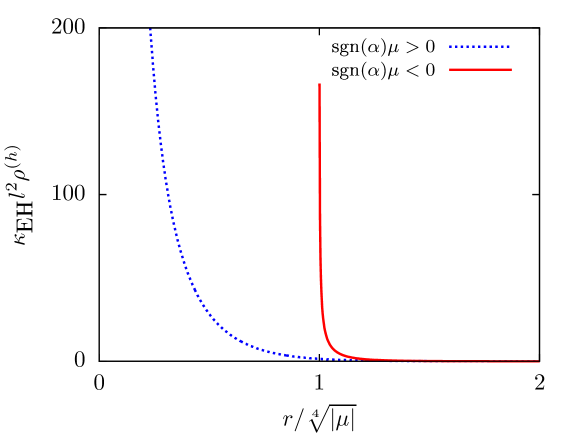
Figure 1: The energy density associated with the field $h^{a}$ ($\beta=1$).

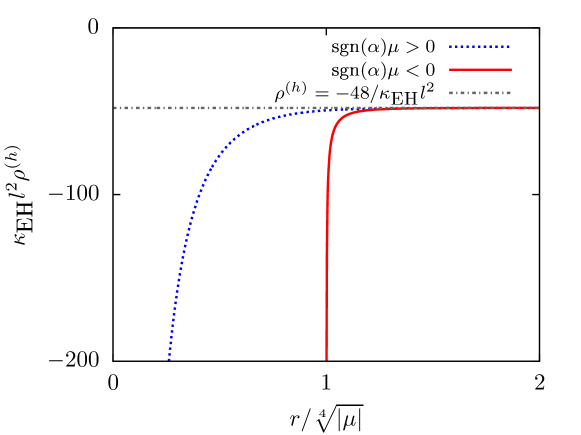
Figure 2: The energy density associated with the field $h^{a}$ ($\beta=-1$).

III.5 Tangential pressures

We can see that the tangential pressures given in the eq. (35) vanishes if

$$\text{sgn}(\alpha)\frac{\mu}{r^{4}}=9+4\beta\sqrt{6}.$$

Thus we have

• If $\beta=1,$ the tangential pressure vanishes only if $\text{sgn}(\alpha)\mu$ is greater than zero (see figure 3).

• If $\beta=-1$ the tangential pressure vanishes only if $\text{sgn}(\alpha)\mu$ is less than zero (see figure 4).

• In other cases, the tangential pressure does not change sign.

Furthermore, it is straightforward to show that there is only one critical point at $r=\sqrt[4]{\frac{\text{sgn}(\alpha)\mu}{5}}$ only if $\mathrm{sgn}(\alpha)\mu>0$.

III.5.1 Case $\beta=1$

If $\beta=1,$ three cases are distinguished, depending on the quantity $\mathrm{sgn}(\alpha)\mu$

1. For $\mu=0$, we have the simplest case. The tangential pressure is zero for all $r$ .

2. If $\mathrm{sgn}(\alpha)\mu>0,$ the tangential pressure diverges at $r=0$.  It is a function that tends to $-\infty$ at $r=0$, vanishes at

   $$r_{1}=\sqrt[4]{\text{sgn}(\alpha)\mu\,\frac{4\sqrt{6}-9}{15}}\approx 0.48\sqrt[4]{|\mu|},$$ (37)

   takes its maximum value

   $$p_{i}^{(h)\,\text{max}}=\frac{4}{9\ l^{2}\kappa_{\text{EH}}}\left(54-19\sqrt{6}\right)\approx\frac{3.3}{\ l^{2}\kappa_{\text{EH}}}$$

   at

   $$r_{2}=\sqrt[4]{\frac{\text{sgn}(\alpha)\mu}{5}}\approx 0.67\sqrt[4]{|\mu|}$$ (38)

   and decreases to zero when $r$ tends to infinity.

3. If $\mathrm{sgn}(\alpha)\mu<0$, then the tangential pressure tends to $+\infty$ at

   $$r_{m}=\sqrt[4]{-\text{sgn}(\alpha)\mu}=\sqrt[4]{|\mu|}.$$

   Of course, the manifold is not defined for $r<r_{m}$ (see the metric coefficients in eq. (27)). The tangential pressure is a decreasing function of $r$ which vanishes at infinity, but always greater than zero.

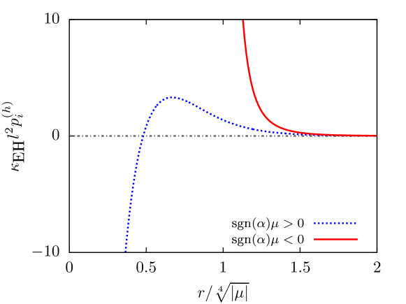
Figure 3: The tangential pressures associated with the field $h^{a}$ ($\beta=1$).

III.5.2 Case $\beta=-1$

If $\beta=-1$ three situations are also distinguished

1. For $\mu=0$, we have the simplest case. The tangential pressure is constant and greater than zero for all $r$

   $$p_{i}^{(h)}(r)=\frac{48}{l^{2}\kappa_{\text{EH}}}.$$

2. If $\mathrm{sgn}(\alpha)\mu>0$, the tangential pressure diverges to positive infinity at $r=0,$ is a decreasing function of $r$, reaches a minimum value

   $$p_{i}^{(h)\,\text{min}}=\frac{4}{9\ l^{2}\kappa_{\text{EH}}}\left(54+19\sqrt{6}\right)\approx\frac{45}{\ l^{2}\kappa_{\text{EH}}}$$

   at

   $$r=\sqrt[4]{\frac{\text{sgn}(\alpha)\mu}{5}}\approx 0.67\sqrt[4]{|\mu|},$$

   and then increases to a bounded infinite value

   $$p_{i}^{(h)}(r\rightarrow\infty)=\frac{48}{l^{2}\kappa_{\text{EH}}}.$$

   The tangential pressure is always greater than zero.

3. If $\mathrm{sgn}(\alpha)\mu<0,$ the tangential pressure diverges to negative infinity at (remember that the manifold is not defined for $r<r_{m}$)

   $$r_{m}=\sqrt[4]{-\text{sgn}(\alpha)\mu}=\sqrt[4]{|\mu|}.$$

   The tangential pressure is an increasing function of $r$ which tends to a positive constant value when $r$ goes to infinity

   $$p_{i}^{(h)}(r\rightarrow\infty)=\frac{48}{l^{2}\kappa_{\text{EH}}}.$$

   Furthermore, the tangential pressures become zero at

   $$\quad r=\sqrt[4]{-\text{sgn}(\alpha)\mu\,\frac{9+4\sqrt{6}}{15}}\approx 1.06\sqrt[4]{|\mu|}.$$

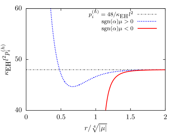
Figure 4: The tangential pressures associated with the field $h^{a}$ ($\beta=-1$).

IV Spherically Symmetric Solution from General Solution

Now consider the case of spherically symmetric solutions studied in Ref. salg4 and reviewed in section II. These solutions are described by the vielbein defined in eq. (11) with the functions $f(r)$ and $g(r)$ given in eq. (12).

This solution corresponds to the general static solution found in (27) where (i) the curvature of the so called, three-dimensional base manifold, is taken positive $\gamma=1$ (sphere $S^{3}$), (ii) the constant $\mu$, written in terms of the mass $M$ of the distribution is given by $$\mu=\frac{\kappa_{EH}}{6\pi^{2}}Ml^{2}>0,$$ (iii) and $\beta=1$ so that this solution has as limit when $l\rightarrow 0$, the 5D Schwarzschild black hole obtained from the Einstein Hilbert gravity.

From Ref. salg4 , we know that the relative values of the mass $M$ and the distance $l$ of this solution leads to black holes or naked singularities.

1. In the event that $\alpha>0$, the manifold only has one singularity at $r=0$. Otherwise, if $\alpha<0$, the manifold has only one singularity at

   $$r_{m}=\sqrt[4]{\mu}=\sqrt[4]{\frac{\kappa_{\mathrm{EH}}}{6\pi^{2}}Ml^{2}}.$$ (39)

2. There is a black hole solution with event horizon defined by

   $$r_{0}=\sqrt{\frac{\mu-\text{sgn}(\alpha)\,l^{4}}{2l^{2}}}=\sqrt{\frac{\kappa_{\text{EH}}}{12\pi^{2}}M-\text{sgn}(\alpha)\frac{l^{2}}{2}},$$ (40)

   if $\mu>l^{4}$, or equivalently

   $$\frac{\kappa_{\mathrm{EH}}}{6\pi^{2}}M>l^{2}.$$ (41)

   Otherwise, there is a naked singularity.

IV.1 Case $\alpha>0$

In this case the energy density appears to be decreasing and vanishes at infinity and the radial pressure behaves reversed (see subsection III.4 with $\beta=1$ and $\mathrm{sgn}(\alpha)\,\mu>0$).

Much more interesting is the behavior of the tangential pressure. In fact, as we already studied in subsection III.5, the tangential pressure is less than zero for $r<r_{1}$ (37), vanishes at $r_{1}$, becomes greater than zero until reaching a maximum at $r_{2}$ (38) and then decreases until it becomes zero at infinity.

IV.1.1 Comparison between $r_{0}$, $r_{1}$ and $r_{2}$ for black hole solution

When the solution found is a black hole, then it must satisfy the condition (41) and has event horizon in $r_{0}$ given in (40). It may be of interest to study the cases when $r_{0}$ is larger or smaller than $r_{1}$ and $r_{2}$.

First consider $r_{0}$ for $l$ fixed, i.e., we study the behavior of the $r_{0}=r_{0}(\mu)$ function. For $\mu\geq l^{4}$ (black hole solution), $r_{0}=r_{0}(\mu)$ is a well-defined, continuous and strictly increasing function of $\mu$ which has an absolute minimum at $\mu=l^{4}$, where it vanishes, i.e., $r_{0}(\mu=l^{4})=0$. Furthermore, when $\mu\gg l^{4}$ the $r_{0}(\mu)$ function behaves like $\sqrt{\mu}$.

On the other hand, the study of functions $r_{1}(\mu)$ and $r_{2}(\mu)$ shows that they are well defined, continuous and strictly increasing functions of $\mu\geq 0$ which vanish at $\mu=0$. As $\mu$ increases, $r_{1}$ and $r_{2}$ grow proportional to $\sqrt[4]{\mu}$.

From the definitions of $r_{1}$ and $r_{2}$ given in eqs. (37) and (38), and the preceding analysis, it follows that $r_{2}>r_{1}>r_{0}$ if $\mu=l^{4}$, and $r_{0}>r_{2}>r_{1}$ if $\mu\rightarrow\infty$. This means that should exist a unique value of the constant $\mu$, denoted $\mu_{1}$ such that $r_{0}(\mu_{1})=r_{1}(\mu_{1})$ and a single $\mu_{2}$ such that $r_{0}(\mu_{2})=r_{2}(\mu_{2})$. After some calculations is obtained

$$\mu_{1}=\frac{l^{4}}{15}\left(8\sqrt{6}-3+2\sqrt{6\left(7-2\sqrt{6}\right)}\right)\approx 1.58\ l^{4}$$

and

$$\mu_{2}=\frac{l^{4}}{5}\left(7+2\sqrt{6}\right)\approx 2.38\ l^{4}.$$

From the above analysis it is concluded that depending on the value of the constant $\mu$, proportional to the mass, we could have the following cases

• If $l^{4}\leq\mu<\mu_{1}$ then $r_{0}<r_{1}$. Outside the black hole horizon, there is a region $r_{0}<r<r_{1}$ where the tangential pressure is negative.

• If $\mu>\mu_{1}$ then $r_{0}>r_{1}$, the zone in which the tangential pressure is negative is enclosed within the black hole horizon.

A completely analogous analysis can be done to study the relationship between $r_{0}$ and $r_{2}$: if $\mu<\mu_{2}$, the maximum value of the tangential pressure is outside the event horizon or, inside if $\mu>\mu_{2}$.

IV.1.2 Pressure radial and tangential pressures

In summary, for $\alpha>0$ we can see that the energy density is always greater than zero, while the radial pressure is less than zero, both vanish when $r$ goes to infinity (see figure 5).

On the other hand, the lateral pressures are less than zero for $r<r_{1}$, become positive for $r>r_{1}$ reaching a maximum at $r_{2}$ and then decrease until vanish when $r$ goes to infinity (see figure 5).

The solution may be a naked singularity $(\mu<l^{4})$ or a black hole $(\mu>l^{4})$. In case of a black hole there is an event horizon at $r=r_{0}$, which can hide the zone of negative tangential pressures ($\mu>\mu_{1}$) or otherwise, remains uncovered.

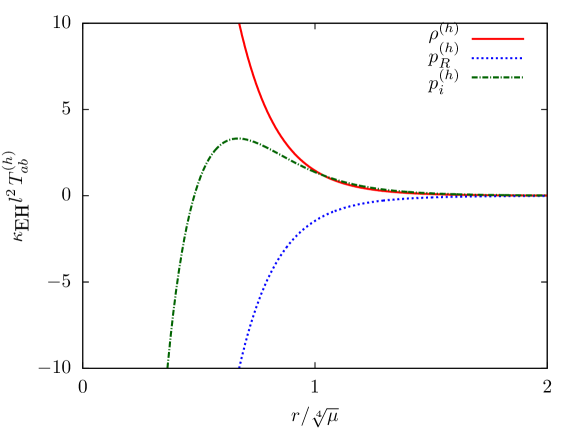
Figure 5: The components of energy-momentum tensor associated with the field $h^{a}$ ($\alpha>0$). Note the interesting behavior of tangential pressure: is negative for $r<r_{1}$, vanishes at $r_{1}$, reaches a maximum at $r_{2}$ and then decreases to zero at infinity. The energy density and pressures tend rapidly to zero as $1/r^{8}$.

IV.2 Case $\alpha<0$

Now consider the coupling constant $\alpha<0$. In this case the space-time has a minimum radius $r_{m}$, defined in (39), where is located the singularity.

From analysis done in subsection III.4 (with $\beta=1$ and $\mathrm{sgn}(\alpha)\,\mu<0$) we obtain that the energy density is progressively reduced and vanishes at infinity. On the other hand, the radial pressure is just the negative energy density (see figure 6).

Furthermore, the tangential positive pressure tends to infinity at $r=r_{m}=\sqrt[4]{\mu}$ and decreases to zero at infinity (see subsection III.5 with $\beta=1$ and $\mathrm{sgn}(\alpha)\,\mu<0$).

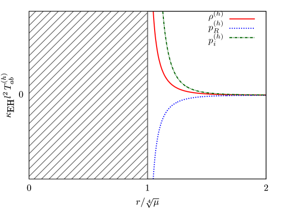
Figure 6: The components of energy-momentum tensor associated with the field $h^{a}$ ($\alpha<0$). The space time singularity is located at $r_{m}=\sqrt[4]{\mu}$. The region $r<r_{m}$ does not belong to the variety. As in case $\alpha>0$ (see figure 5), the energy density and pressures tend to zero as $1/r^{8}$.

V Concluding Remarks

An interesting result of this work is that when the field $h^{a}$, which appears in the Lagrangian (1), is modeled as an anisotropic fluid (see eqs. (34 - 35)), we find that the solutions of the fields equations predicts the existence of a negative tangential pressure zone around low-mass distributions ($\mu<\mu_{1}$) when the coupling constant $\alpha$ is greater than zero.

Additionally ($\alpha>0$), this model predicts the existence of a maximum in the tangential pressure, which can be observed in the outer region of a field distribution that satisfies $\mu<\mu_{2}$.

It is also important to note that this model contains in its solutions space, solutions that behave like those obtained from models with negative cosmological constant ($\beta=-1$). In such a situation, the field $h^{a}$ is playing the role of a cosmological constant GMS ; salg5 .

In this article we have assumed that the matter Lagrangian $L_{M}$ satisfies the property $\delta L_{M}/\delta e^{a}=0$ and that the energy-momentum tensor associated to the $h^{a}$ field can be modeled as an anisotropic fluid. A possible explicit example of the matter Lagrangian which satisfies these considerations could be constructed from a Lagrangian of the electromagnetic field in matter 11 ; 12 ; 13 . In fact, a candidate for matter Lagrangian which satisfies the above conditions would be

$$L_{M}=-\frac{1}{2}\,\frac{1}{4!}\,\epsilon_{cdmnl}F_{ab}H^{cd}h^{a}h^{b}h^{m}h^{n}h^{l},$$

where $F_{ab}$ is the electromagnetic field and $H^{cd}$ is the so called electromagnetic exitation, which is given by (in tensorial notation)

$$H^{\mu\nu}=\frac{1}{2}\chi^{\mu\nu\rho\sigma}F_{\rho\sigma},$$

where the tensor density $\chi^{\mu\nu\rho\sigma}$ describes the electric and magnetic properties of matter.

Appendix A Obtaining the energy-momentum tensor associated to the field $h^{a}$

In this appendix we show explicitly the computations that lead to obtain the energy density and pressures associated to the field $h^{a}$ shown in eqs. (34) and (35) from the field equation (9).

The field equation (9) can be rewritten as

$$-\frac{l^{2}}{2\kappa_{\text{EH}}}\text{sgn}(\alpha)\star\left(\epsilon_{abcde}R^{bc}R^{de}\right)=\hat{T}_{ab}^{(h)}e^{b},$$ (42)

where we see it is necessary to compute the components of the left side. Straightforward calculations lead to

$$\star\left(\epsilon_{Tbcde}R^{bc}R^{de}\right) =6\ \frac{\left\{(g^{2}-\gamma)^{2}\right\}^{\prime}}{r^{3}}\ e^{T},$$ (43)

$$\star\left(\epsilon_{Rbcde}R^{bc}R^{de}\right) =-6\ \frac{\left\{(g^{2}-\gamma)^{2}\right\}^{\prime}}{r^{3}}\ e^{R},$$ (44)

$$\star\left(\epsilon_{ibcde}R^{bc}R^{de}\right) =-2\ \frac{\left\{(g^{2}-\gamma)^{2}\right\}^{\prime\prime}}{r^{2}}\ e^{i}.$$ (45)

From the general solution found in eq. (27) we obtain

$$(g^{2}-\gamma)^{2}=\frac{r^{4}}{l^{4}}\left(2+\text{sgn}(\alpha)\frac{\mu}{r^{4}}-2\beta\sqrt{1+\text{sgn}(\alpha)\frac{\mu}{r^{4}}}\right),$$ (46)

so that

$$\bigl{\{}(g^{2}-\gamma)^{2}\bigr{\}}^{\prime}=4\frac{r^{3}}{l^{4}}\left\{2-\beta\frac{2+\text{sgn}(\alpha)\frac{\mu}{r^{4}}}{\sqrt{1+\text{sgn}(\alpha)\frac{\mu}{r^{4}}}}\right\}$$ (47)

and

$$\bigl{\{}(g^{2}-\gamma)^{2}\bigr{\}}^{\prime\prime}=4\frac{r^{2}}{l^{4}}\left\{6-\beta\,\frac{6+9\,\text{sgn}(\alpha)\frac{\mu}{r^{4}}+\frac{\mu^{2}}{r^{8}}}{\left(1+\text{sgn}(\alpha)\frac{\mu}{r^{4}}\right)^{\frac{3}{2}}}\right\},$$ (48)

where we realize that none of those last three terms depend on the $\gamma$ constant.

Hence, by replacing eqs. (47) and (48) into eqs. (43 - 45) and then into eq. (42), we get

$$\rho^{(h)}(r) =-p_{R}^{(h)}(r)=-\frac{12}{l^{2}\kappa_{\text{EH}}}\left\{2-\beta\frac{2+\text{sgn}(\alpha)\frac{\mu}{r^{4}}}{\sqrt{1+\text{sgn}(\alpha)\frac{\mu}{r^{4}}}}\right\},$$

$$p_{i}^{(h)}(r) =\frac{4}{l^{2}\kappa_{\text{EH}}}\left\{6-\beta\,\frac{6+9\,\text{sgn}(\alpha)\frac{\mu}{r^{4}}+\frac{\mu^{2}}{r^{8}}}{\left(1+\text{sgn}(\alpha)\frac{\mu}{r^{4}}\right)^{\frac{3}{2}}}\right\},$$

where we have introduced the energy-momentum tensor associated to the field $h^{a}$ given in eq. (33).

References

- (1) F. Izaurieta, P. Minning, A. Perez, E. Rodriguez and P. Salgado, Standard general relativity from Chern-Simons gravity, Phys. Lett. B 678 (2009) 213–217, [arXiv:0905.2187].
- (2) F. Izaurieta, E. Rodríguez and P. Salgado, Expanding Lie (super)algebras through Abelian semigroups, J. Math. Phys. 47 (2006) 123512, [arXiv:hep-th/0606215].
- (3) F. Izaurieta, A. Perez, E. Rodriguez and P. Salgado, Dual formulation of the Lie algebra S-expansion procedure, J. Math. Phys. 50 (2009) 073511, [arXiv:0903.4712].
- (4) C. A. C. Quinzacara and P. Salgado, Black hole for the Einstein-Chern-Simons gravity, Phys. Rev. D 85 (2012) 124026, [arXiv:1401.1797].
- (5) G. Dotti, J. Oliva and R. Troncoso, Exact solutions for the Einstein-Gauss-Bonnet theory in five dimensions: Black holes, wormholes, and spacetime horns, Phys. Rev. D 76 (2007) 064038, [arXiv:0706.1830].
- (6) J. Oliva, All the solutions of the form for Lovelock gravity in vacuum in the Chern-Simons case, J. Math. Phys. 54 (2013) 042501, [arXiv:1210.4123].
- (7) G. Gibbons and S. A. Hartnoll, Gravitational instability in higher dimensions, Phys. Rev. D 66 (2002) 064024, [arXiv:hep-th/0206202].
- (8) C. A. C. Quinzacara and P. Salgado, Stellar equilibrium in Einstein-Chern-Simons gravity, Eur. Phys. J. C 73 (2013) 2479, [arXiv:1607.07533].
- (9) F. Gomez, P. Minning and P. Salgado, Standard cosmology in Chern-Simons gravity, Phys. Rev. D 84 (2011) 063506.
- (10) M. Cataldo, J. Crisóstomo, S. del Campo, F. Gómez, C. C. Quinzacara and P. Salgado, Accelerated FRW solutions in Chern-Simons gravity, Eur. Phys. J. C 74 (2014) 3087, [arXiv:1401.2128].
- (11) Y. Obukhov, Electromagnetic energy and momentum in moving media, Ann. Phys. 17 (2008) 830–851, [arXiv:0808.1967].
- (12) T. Ramos, G. F. Rubilar and Y. N. Obukhov, First principles approach to the Abraham–Minkowski controversy for the momentum of light in general linear non-dispersive media, J. Opt. 17 (2015) 025611, [arXiv:1310.0518].
- (13) Y. N. Obukhov, T. Ramos and G. F. Rubilar, Relativistic Lagrangian model of a nematic liquid crystal interacting with an electromagnetic field, Phys. Rev. E 86 (2012) 031703, [arXiv:1203.3122].