Paths of zeros of analytic functions describing finite quantum systems

Abstract

Quantum systems with positions and momenta in ${\mathbb{Z}}(d)$, are described by the $d$ zeros of analytic functions on a torus. The $d$ paths of these zeros on the torus, describe the time evolution of the system. A semi-analytic method for the calculation of these paths of the zeros, is discussed. Detailed analysis of the paths for periodic systems, is presented. A periodic system which has the displacement operator to a real power $t$, as time evolution operator, is studied. Several numerical examples, which elucidate these ideas, are presented.

1 Introduction

There is an extensive literature on analytic representations in quantum mechanics, after the pioneering work by Bargmann [1, 2]. The Bargmann analytic function in the complex plane studies problems related to the harmonic oscillator. The zeros of the Bargmann function, which are also the zeros of the Husimi (or $Q$) function, provide a valuable insight to various quantum systems [3, 4, 5, 6, 7, 8, 9, 10], chaos [10], etc. Other potential applications include the study of two-dimensional electron gas in a magnetic field, quantum Hall effect, [11, 12, 13], etc.

Analytic representations in the unit disc for problems with $SU(1,1)$ symmetry, and analytic representations in the extended complex plane for systems with $SU(2)$ symmetry, have also been studied in the literature (reviews have been presented in [14, 15, 16]).

Quantum systems with variables in ${\mathbb{Z}}(d)$ (the integers modulo $d$), have been studied extensively in the literature (e.g., [17, 18, 19, 20]). Refs.[21, 22, 25, 23, 24] have represented their quantum states with analytic functions on a torus, using Theta functions. It has been shown that these functions have exactly $d$ zeros, which determine uniquely the state of the system. As the system evolves in time, the zeros follow $d$ paths, on the torus. Ref [4] has also used a similar representation in studies of chaos. Theta functions have been used extensively in various problems in physics [26, 27].

In this paper we study different aspects of the zeros of analytic functions for finite quantum systems with variables in ${\mathbb{Z}}(d)$, as follows:

• We propose in Eqs.(18),(19) a semi-analytic method for the calculation of the paths of the zeros, which is primarily analytical (section 2). Previous work is based on entirely numerical methods. In principle the full quantum formalism can be expressed in terms of the $d$ zeros. But it is difficult to express physical laws in terms of the zeros, without an analytical formalism that relates physical quantities with the zeros. The semi-analytical formalism in this paper, is a step in this direction.

• We study in detail the $d$ paths of the zeros of periodic systems. Each path is characterized by the multiplicity M, and by a pair of winding numbers $(w_{1},w_{2})$. An interesting periodic system is one, which has as time evolution operator the displacement operator to a real power $t$. Displacement operators ${\cal Z}^{\alpha}{\cal X}^{\beta}$ are defined in finite quantum systems for $\alpha,\beta\in{\mathbb{Z}}(d)$, and it is interesting to study these operators to a real power $t$. It is shown that the paths of the zeros are identical, but shifted with respect to each other (section 3).

2 Analytic representation of finite quantum systems

We consider a finite quantum system with variables in ${\mathbb{Z}}(d)$. This system is described with the $d$-dimensional Hilbert space ${\cal H}(d)$. Let $|X;m\rangle$ and $|P;m\rangle$ (where $m\in{\mathbb{Z}}(d)$) be the position and momentum bases which are related through a Fourier transform, as follows:

$$|P;n\rangle={\cal F}|{X};n\rangle;\qquad{\cal F}=d^{-1/2}\sum_{m,n}\omega(mn)|X;m\rangle\langle X;n|;$$

$$\omega(m)=\exp\left[i\frac{2\pi m}{d}\right]$$ (1)

Let $|g\rangle$ be an arbitrary state

$$|g\rangle=\sum_{m}g_{m}|X;m\rangle;\qquad\sum_{m}|g_{m}|^{2}=1$$ (2)

We use the notation

$$|g^{*}\rangle=\sum_{m}g_{m}^{*}|X;m\rangle;\;\;\langle g|=\sum_{m}g_{m}^{*}\langle X;m|$$

$$\langle g^{*}|=\sum_{m}g_{m}\langle X;m|$$ (3)

We represent the state $|g\rangle$ with the analytic function [3, 4, 21]

$$G(z)=\pi^{-1/4}\sum_{m=0}^{d-1}g_{m}\;\Theta_{3}\left[\frac{\pi m}{d}-z\sqrt{\frac{\pi}{2d}};\frac{i}{d}\right]$$ (4)

where $\Theta_{3}$ is the Theta function [28]

$$\Theta_{3}(u,\tau)=\sum_{n=-\infty}^{\infty}\exp(i\pi\tau n^{2}+i2nu)$$

$$\Theta_{3}^{\prime}(u,\tau)=\frac{{\rm d}\Theta_{3}}{{\rm d}u}=i\sum_{n=-\infty}^{\infty}2n\exp(i\pi\tau n^{2}+i2nu).$$ (5)

We can prove that

$$G(z+\sqrt{2\pi d})=G(z)$$

$$G(z+i\sqrt{2\pi d})=G(z)\exp\left(\pi d-iz\sqrt{2\pi d}\right),$$ (6)

and therefore it is sufficient to have this function in a cell

$$S=[M\sqrt{2\pi d},(M+1)\sqrt{2\pi d})\times[N\sqrt{2\pi d},(N+1)\sqrt{2\pi d})$$ (7)

where $(M,N)$ are integers labelling the cell. Other models with more general quasi-periodic boundary conditions can also be studied. The scalar product is given by

$$\langle f^{\ast}|g\rangle=\frac{1}{d^{3/2}\sqrt{2\pi}}\int_{S}{\rm d}\mu(z)F(z^{*})G(z)=\sum f_{m}g_{m};$$

$${\rm d}\mu(z)={\rm d}^{2}z\exp\left(-z_{I}^{2}\right)$$ (8)

These relations are proved using the orthogonality relation[22]

$$2^{-1/2}\pi^{-1}d^{-3/2}\int_{S}{\rm d}\mu(z) \Theta_{3}\left[\frac{\pi n}{d}-z\sqrt{\frac{\pi}{2d}};\frac{i}{d}\right]$$

$$\times\Theta_{3}\left[\frac{\pi m}{d}-z^{*}\sqrt{\frac{\pi}{2d}};\frac{i}{d}\right]=\delta(m,n)$$ (9)

The coefficients $g_{m}$ in Eq.(2) are given by

$$g_{m}=2^{-1/2}\pi^{-3/4}d^{-3/2}\int_{S}{\rm d}\mu(z)\Theta_{3}\left[\frac{\pi m}{d}-z\sqrt{\frac{\pi}{2d}};\frac{i}{d}\right]G(z^{*}).$$ (10)

It has been proved in [4, 21] that the analytic function $G(z)$ has exactly $d$ zeros $\zeta_{n}$ in each cell $S$, and that

$$\sum_{n=1}^{d}\zeta_{n}=\sqrt{2\pi d}(M+iN)+d^{3/2}\sqrt{\frac{\pi}{2}}(1+i).$$ (11)

in finite systems the $d-1$ zeros define uniquely the state (the last zero is determined from Eq.(11)). In infinite systems the zeros do not define uniquely the state.

If the $d-1$ zeros $\zeta_{n}$ are given, the last one can be found from Eq.(11), and the function $G(z)$ is given by

$$G(z)={\cal N}(\{\zeta_{n}\})$$

$$\times\exp\left[-i\sqrt{\frac{2\pi}{d}}Nz\right]\prod_{n=1}^{d}\Theta_{3}\left[\sqrt{\frac{\pi}{2d}}(z-\zeta_{n})+\frac{\pi(1+i)}{2};\;i\right]$$ (12)

Here $N$ is the integer that labels the cell (as in Eq.(7)), and ${\cal N}(\{\zeta_{n}\})$ is a normalization constant that does not depend on $z$ (see section 7 in ref[21]). Below we choose the cell with $M=N=0$.

2.1 Time evolution and paths of zeros

Let $H$ be the Hamiltonian of the system (a $d\times d$ Hermitian matrix $H_{mn}$). As the system evolves in time $t$, each zero $\zeta_{n}$ follows a path $\zeta_{n}(t)$.

We consider infinitesimal changes to the coefficients from $g_{m}$ to $g_{m}+\Delta g_{m}$, where

$$\Delta g_{m}=i\Delta t\sum_{n}H_{mn}g_{n}$$ (13)

Then the zeros will change from $\zeta_{n}$ to $\zeta_{n}+\Delta\zeta_{n}$. From Eqs.(4),(2) we get

$$\pi^{-1/4}\sum_{m=0}^{d-1}(g_{m}+\Delta g_{m})\;\Theta_{3}\left[\frac{\pi m}{d}-z\sqrt{\frac{\pi}{2d}};\frac{i}{d}\right]$$

$$={\cal N}(\{\zeta_{k}\})\prod_{n=1}^{d}\Theta_{3}\left[\sqrt{\frac{\pi}{2d}}(z-\zeta_{n}-\Delta\zeta_{n})+\frac{\pi(1+i)}{2};\;i\right]$$ (14)

With a Taylor expansion of the right hand side, we get

$$\pi^{-1/4}\sum_{m=0}^{d-1}\Delta g_{m}\;\Theta_{3}\left[\frac{\pi m}{d}-z\sqrt{\frac{\pi}{2d}};\frac{i}{d}\right]=-{\cal N}(\{\zeta_{k}\})\sqrt{\frac{\pi}{2d}}$$

$$\times\sum_{j=1}^{d}A_{j}(z)\Theta_{3}^{\prime}\left[\sqrt{\frac{\pi}{2d}}(z-\zeta_{j})+\frac{\pi(1+i)}{2};\;i\right]\Delta\zeta_{j}$$

$$A_{j}(z)=\prod_{m\neq j}\Theta_{3}\left[\sqrt{\frac{\pi}{2d}}(z-\zeta_{m})+\frac{\pi(1+i)}{2};\;i\right]$$ (15)

We insert $z=\zeta_{n}$ on both sides of this equation. For $j\neq n$ we get $A_{j}(\zeta_{n})=0$. Therefore

$$\pi^{-1/4}\sum_{m=0}^{d-1}\Delta g_{m}\;\Theta_{3}\left[\frac{\pi m}{d}-\zeta_{n}\sqrt{\frac{\pi}{2d}};\frac{i}{d}\right]$$

$$=-{\cal N}(\{\zeta_{k}\})\sqrt{\frac{\pi}{2d}}A_{n}(\zeta_{n})\Theta_{3}^{\prime}\left[\frac{\pi(1+i)}{2};\;i\right]\Delta\zeta_{n}$$

$$A_{n}(\zeta_{n})=\prod_{m\neq n}\Theta_{3}\left[\sqrt{\frac{\pi}{2d}}(\zeta_{n}-\zeta_{m})+\frac{\pi(1+i)}{2};\;i\right]$$ (16)

Using Eq.(2), we found numerically that

$$\Theta_{3}^{\prime}\left[\frac{\pi(1+i)}{2};\;i\right]=1.9888i.$$ (17)

Therefore we have analytical expressions for the derivatives of the functions $\zeta_{n}(g_{0},...,g_{d-1})$:

$$\frac{\partial\zeta_{n}}{\partial g_{m}}=-\frac{\pi^{-1/4}\Theta_{3}\left[\frac{\pi m}{d}-\zeta_{n}\sqrt{\frac{\pi}{2d}};\frac{i}{d}\right]}{{\cal N}(\{\zeta_{k}\})\sqrt{\frac{\pi}{2d}}A_{n}(\zeta_{n})\Theta_{3}^{\prime}\left[\frac{\pi(1+i)}{2};\;i\right]}$$ (18)

We use them for numerical calculations as

$$\zeta_{n}+\Delta\zeta_{n}=\zeta_{n}+\sum_{m}\frac{\partial\zeta_{n}}{\partial g_{m}}\Delta g_{m}=\zeta_{n}+i\Delta t\sum_{m,k}\frac{\partial\zeta_{n}}{\partial g_{m}}H_{mk}g_{k}.$$ (19)

In each step of the iteration process ${\cal N}(\{\zeta_{k}\})$ is calculated as

$${\cal N}(\{\zeta_{k}\})=\frac{\pi^{-1/4}\sum_{m=0}^{d-1}g_{m}\;\Theta_{3}\left[\frac{\pi m}{d}-z\sqrt{\frac{\pi}{2d}};\frac{i}{d}\right]}{\prod_{n=1}^{d}\Theta_{3}\left[\sqrt{\frac{\pi}{2d}}(z-\zeta_{n})+\frac{\pi(1+i)}{2};\;i\right]}$$ (20)

and is used in the next step. As we mentioned earlier, the ${\cal N}(\{\zeta_{k}\})$ does not depend on $z$ and any value of $z$ can be used for its numerical calculation. Since $\sum_{m}|g_{m}|^{2}=1$ the $\Delta g_{m}$ are subject to the constraint

$$\sum_{m}[g_{m}^{*}\Delta g_{m}+g_{m}(\Delta g_{m})^{*}]=0.$$ (21)

Ref[22] calculated the paths of the zeros indirectly, using a computationally expensive approach. It calculated the vector $\exp(itH)|f\rangle$ and then the analytic function $f(z;t)$, at each time $t$. Then a MATLAB function was used to find the zeros, at each time $t$.

In all calculations of the present paper, we go directly from the zero $\zeta_{n}(t)$ to the zero $\zeta_{n}(t+\Delta t)$ with Eqs.(18),(19). For the calculation of ${\cal N}(z;\{\zeta_{n}\})$ we need the coefficients $g_{m}$ at each step. At $t=0$ we start from given values of zeros, which we insert in Eq.(4) and get a system of $d$ equations with $d$ unknowns. This gives the coefficients $g_{m}$ at $t=0$ (which we normalize). At later times the $g_{m}$ becomes $g_{m}+\Delta g_{m}$, where $\Delta g_{m}$ is the step used in Eqs.(13),(19). The present method is semi-analytic and therefore computationally less expensive and more accurate.

3 Periodic systems

We consider periodic systems with Hamiltonians such that $\exp(iTH)={\bf 1}e^{i\theta}$ for some $T$, and some phase factor $e^{i\theta}$ (which does not change the physical state). This occurs when the ratios of the eigenvalues of $H$ are rational numbers.

Results analogous to those in sections 3.1-3.3, have been reported in ref[22], using an entirely numerical method. Our results here are based on the semi-analytical method described in section 2.

3.1 Multiplicity $M$ of paths of zeros:

We consider the Hamiltonian

$$H=\begin{bmatrix}1&1&0&0\\ 1&1&0&0\\ 0&0&1&0\\ 0&0&0&1\end{bmatrix}$$ (22)

In this case the period is $T=2\pi$. We assume that at $t=0$ the zeros are the following:

$$\zeta_{0}(0)=1-1.99i; \zeta_{1}(0)=3.02+3i;\quad$$

$$\zeta_{2}(0)=1+3i; \zeta_{3}(0)=-0.01+1i.$$ (23)

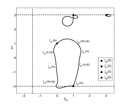
Figure 1: Paths of the zeros for the Hamiltonian of Eq.(22). The period is $T=2\pi$. At $t=0$ the zeros are given in Eq.(3.1). Dotted lines show a cell, which is a square with each side equal to $5.01$

Using Eq.(19) we have calculated the paths of the zeros. Results are shown in Fig.1 (see also Fig.4 in ref[22]). In this case there are two paths with multiplicity $M=1$ and one path with multiplicity $M=2$. For clarity, the figures show regions which might be larger or smaller than one cell (which is a square with each side equal to $\sqrt{2\pi d}$). They also show the position of the zeros at various times. We note that

$$\zeta_{0}(T)=\zeta_{3}(0); \zeta_{3}(T)=\zeta_{0}(0)\quad$$

$$\zeta_{1}(0)=\zeta_{1}(T); \zeta_{2}(0)=\zeta_{2}(T).$$ (24)

It is seen that although the set of zeros has period $T$, a particular zero (e.g., $\zeta_{0}$ or $\zeta_{3}$) returns to its original position after time which is a multiple of $T$ (in this example $2T$).

We also consider the Hamiltonian of Eq.(22) and assume that at $t=0$ the zeros are

$$\zeta_{0}(0)=2-2.99i; \zeta_{1}(0)=2.02-2.01i;\quad$$

$$\zeta_{2}(0)=1-1.01i; \zeta_{3}(0)=-0.01+i;\quad$$ (25)

in which case the results are shown in Fig.2. In this case we have one path with multiplicity $M=4$. Here

$$\zeta_{0}(T)=\zeta_{2}(0); \zeta_{2}(T)=\zeta_{3}(0)\quad$$

$$\zeta_{3}(T)=\zeta_{1}(0); \zeta_{1}(T)=\zeta_{0}(0).$$ (26)

3.2 Winding numbers $(w_{1},w_{2})$ of paths of zeros:

We consider the Hamiltonian

$$H=\begin{bmatrix}1.5&0.2&0\\ 0.2&1.5&0\\ 0&0&2.1\\ \end{bmatrix}$$ (27)

In this case the period is $T=5\pi$. We assume that at $t=0$ the zeros are the following:

$$\zeta_{0}(0)=1.01+2i;\;\zeta_{1}(0)=2.15+2.56i$$

$$\zeta_{2}(0)=3.35+1.95i.$$ (28)

The paths of zeros are shown in Fig.3. The winding numbers $(w_{1},w_{2})$ of the three paths are $(0,0)$, $(0,1)$ and $(0,1)$.

3.3 Joining of two paths of zeros into a single path:

We consider the Hamiltonian

$$H=\begin{bmatrix}0&1&0&0&0\\ 1&0&0&0&0\\ 0&0&1&0&1\\ 0&0&0&1&1\\ 0&0&1&1&0\\ \end{bmatrix}$$ (29)

In this case the period is $T=2\pi$. We consider two cases where at $t=0$ the zeros are given by

$$\zeta_{0}(0)=1.3+4.16i; \zeta_{1}(0)=0.12+2.03i;$$

$$\zeta_{2}(0)=0.11+1.62i; \zeta_{3}(0)=-2.6-0.2i;$$

$$\zeta_{4}(0)=-1.71+.81i,$$ (30)

and also by

$$\zeta_{0}(0)=1.3+4.16i; \zeta_{1}(0)=0.1+2.0i;$$

$$\zeta_{2}(0)=0.11+1.62i; \zeta_{3}(0)=3-0.2i;$$

$$\zeta_{4}(0)=-1.69+0.83i.$$ (31)

The paths of zeros in these two examples are shown in Figs.4,5, correspondingly. In these figures we see how by changing the initial zeros slightly, two paths (highlighted)with multiplicity $1$, join together into one path (highlighted) with multiplicity $2$.

3.4 Zeros of the analytic representation of ${\cal X}^{t}|g\rangle$

Displacement operators in the ${\mathbb{Z}}(d)\times{\mathbb{Z}}(d)$ phase space, are defined as

$${\cal Z}=\sum_{n}\omega(n)|{X};n\rangle\langle{X};n|$$

$${\cal X}=\sum_{n}\omega(-n)|{P};n\rangle\langle{P};n|$$

$${\cal Z}|{P};n\rangle=|{P};n+1\rangle;\;\;\;\;\;{\cal X}|{X};n\rangle=|{X};n+1\rangle$$

$${\cal X}^{d}={\cal Z}^{d}={\bf 1};\;\;\;\;\;\;{\cal X}^{\beta}{\cal Z}^{\alpha}={\cal Z}^{\alpha}{\cal X}^{\beta}\omega(-\alpha\beta);\;\;\;\;\;\;$$ (32)

where $\alpha,\beta\in{\mathbb{Z}}(d)$. We study the zeros of the analytic representation of ${\cal X}^{t}|g\rangle$ which we denote as $G(z;t)$, where $t\in{\mathbb{R}}$. ${\cal X}^{t}$ can be viewed as a time evolution operator $\exp(itH)$ with Hamiltonian $H=-i\ln{\cal X}$ (the logarithm is multi-valued and we take the principal value).

Let $|g\rangle=\sum{\widetilde{g}}_{m}|P;m\rangle$, where ${\widetilde{g}}_{m}$ are the Fourier transforms of the $g_{m}$ in Eq.(2). The state ${\cal X}^{t}|g\rangle=\sum[\omega(-m)]^{t}{\widetilde{g}}_{m}|P;m\rangle$ is represented by the function

$$G(z;t)=\pi^{-1/4}\exp\left(-\frac{z^{2}}{2}\right)\sum_{m=0}^{d-1}\exp\left(-\frac{i2\pi mt}{d}\right){\widetilde{g}}_{m}$$

$$\times\Theta_{3}\left[\frac{\pi m}{d}-iz\sqrt{\frac{\pi}{2d}};\frac{i}{d}\right]$$ (33)

We used here the fact that the $|P;m\rangle$ is represented by $\pi^{-1/4}\exp\left(-\frac{z^{2}}{2}\right)\Theta_{3}\left[\frac{\pi m}{d}-iz\sqrt{\frac{\pi}{2d}};\frac{i}{d}\right]$[25].

Let $\zeta_{n}(t)$ where $n=0,...,d-1$ be the zeros of $G(z;t)$, i.e.,

$$G[\zeta_{n}(t);t]=0$$ (34)

The index $n$ labels the various paths of zeros.

Proposition 3.1.

Each path of zeros $\zeta_{n+\beta}$ of $G(z;t)$ (that represents ${\cal X}^{t}|g\rangle$), is a shifted version (in the real direction) of another path $\zeta_{n}$. The position of the zero on each path at a certain time, is the same as the position of the zero on another path, at a different time:

$$\zeta_{n+\beta}(t+\beta)=\zeta_{n}(t)+\beta\sqrt{\frac{2\pi}{d}};\;\;\;\;n,\beta\in{\mathbb{Z}}(d).$$ (35)

Proof.

We assume that $G[\zeta_{n}(t);t]=0$ and prove $G[\zeta_{n+\beta}(t+\beta);t+\beta]=0$, where the ‘new path’ $\zeta_{n+\beta}(t+\beta)$ is given in Eq.(35). We express the Theta function as a sum as in Eq.(2) and change the summation from $n\in{\mathbb{Z}}$ into $k_{n}=n-t\in{\mathbb{Z}}-t$. We get

$$G(z;t) = \pi^{-1/4}\exp\left(-\frac{z^{2}}{2}\right)\exp\left(tz\sqrt{\frac{2\pi}{d}}-\frac{\pi t^{2}}{d}\right)$$ (36)

$$\times \sum_{m=0}^{d-1}{\widetilde{g}}_{m}\sum_{k_{n}}\exp\left(\frac{2i\pi mk_{n}}{d}\right)$$

$$\times \exp\left(2k_{n}z\sqrt{\frac{\pi}{2d}}-\frac{\pi k_{n}^{2}}{d}-2\frac{\pi k_{n}t}{d}\right).$$

We insert $z=\zeta_{n+\beta}(t+\beta)$ in $G(z;t)$ and change the variable $t^{\prime}=t-\beta$. Using $G[\zeta_{n}(t);t]=0$ we prove that $G[\zeta_{n+\beta}(t+\beta);t+\beta]=0$. ∎

In fig6 we plot the paths of the zeros of the state $X^{t}|g\rangle$. The state $|g\rangle$ is defined through the zeros at $t=0$ which are

$$\zeta_{0}(0)=1.54+2.47i;\;\zeta_{1}(0)=2.01+2.18i$$

$$\zeta_{2}(0)=2.95+1.86i$$ (37)

It is seen that there are $d$ identical paths, which are shifted in the $z_{R}$-direction by $\sqrt{2\pi/d}$. We note that at a particulat time the zeros do not obey the relation $\zeta_{i+1}(t)=\zeta_{i}(t)+\sqrt{2\pi/d}$ (e.g., the zeros at $t=0$ which are shown in fig7). However, the whole path of a zero over a period, is a shifted version of the path of another zero.

General displacement operators in the ${\mathbb{Z}}(d)\times{\mathbb{Z}}(d)$ phase space, are defined as ${\cal D}(\alpha,\beta)={\cal Z}^{\alpha}{\cal X}^{\beta}\omega(-2^{-1/2})$. In this part of the paper we assume that $d$ is an odd integer, so that $2^{-1}$ exists in ${\mathbb{Z}}(d)$. Let $e_{m}$ and $|u_{m}\rangle$ the eigenvalues and eigenvectors of ${\cal D}(\alpha,\beta)$. We consider the state $|g\rangle=\sum r_{m}|u_{m}\rangle$. We assume that the state $[{\cal D}(\alpha,\beta)]^{t}|g\rangle=\sum e_{m}^{t}|u_{m}\rangle$ is represented by the function ${\mathfrak{G}}(z,t)$. Let $\zeta_{n}(t)$ where $n=0,...,d-1$ be the zeros of ${\mathfrak{G}}(z;t)$, i.e.,

$${\mathfrak{G}}[\zeta_{n}(t);t]=0$$ (38)

We give the following conjecture, which is a generalization of proposition 3.1 for general displacement operators.

Conjecture 3.2.

Each path of zeros of ${\mathfrak{G}}(z,t)$ (that represents $[{\cal D}(\alpha,\beta)]^{t}|g\rangle$), is a shifted version (in both the real and imaginary direction) of another path.

This conjecture is supported with the numerical result in Fig7, where we plot the paths of the zeros of ${\mathfrak{G}}(z,t)$ which represents the state $[{\cal D}(1,1)]^{t}|g\rangle$. The state $|g\rangle$ is defined through the zeros at $t=0$, which are

$$\zeta_{0}(0)=1.4-2.01i;\;\zeta_{1}(0)=2.15+2.32i$$

$$\zeta_{2}(0)=-1.39+1.86i.$$ (39)

4 Discussion

We have considered quantum systems with positions and momenta in ${\mathbb{Z}}(d)$. An analytic representation on a torus that uses Theta functions, which describes these systems, has been given in Eq.(4). The $d$ zeros of these analytic functions define uniquely the state of the system. As the system evolves in time the zeros follow $d$ paths on the torus.

A semi-analytic method for the calculation of these paths of the zeros, has been given in Eqs.(18),(19). It has been used for the study of the paths of periodic systems. Each path is characterized by the multiplicity M, and by a pair of winding numbers $(w_{1},w_{2})$. Other phenomena like the joining of two paths of zeros into a single path, have also been studied. The case that the time evolution operator is the displacement operator to a real power $t$, has also been studied (section 3.4). In this case the paths of the zeros are identical, but shifted with respect to each other.

There are deep links between the zeros of analytic functions and the behaviour of quantum systems. For systems with finite dimensional Hilbert space, the zeros determine the state of the system, and the time evolution can be described with $d$ classical paths on a torus. The ultimate goal is to develop the full quantum formalism in terms of the zeros, and to derive general laws that describe their motion. For example, it is interesting to study what determines the velocity and acceleration of the zeros. Analytical relations between the zeros and the various quantum quantities, would be ideal for this purpose. The semi-analytical method proposed in this paper, is a positive step in this direction.

Other related problems, like the behaviour of the zeros in the semiclassical limit, could also be studied in extensions of the present work.

.

Figure 2: Paths of the zeros for the Hamiltonian of Eq.(22). The period is $T=2\pi$. The zeros at $t=0$ are given in Eq.(3.1).The cell is a square with each side equal to $5.01$

Figure 3: Paths of the zeros for the Hamiltonian of Eq.(27). The period is $T=5\pi$. The zeros at $t=0$ are given in Eq.(3.2). Dotted lines show a cell, which is a square with each side equal to $4.34$

Figure 4: Paths of the zeros for the Hamiltonian of Eq.(29). The period is $T=2\pi$. At $t=0$ the zeros are given in Eq.(3.3). Dotted lines show a cell, which is a square with each side equal to $5.6$

Figure 5: Paths of the zeros for the Hamiltonian of Eq.(29). The period is $T=2\pi$. At $t=0$ the zeros are given in Eq.(3.3). Dotted lines show a cell, which is a square with each side equal to $5.6$

Figure 6: Paths of the zeros of the analytic representation of the state ${\cal X}^{t}|g\rangle$. The period is $T=3$. The state $|g\rangle$ is defined through the zeros at $t=0$ given in Eq.(3.4). Dotted lines show a cell, which is a square with each side equal to $4.34$

Figure 7: Paths of the zeros of the analytic representation of the state $[{\cal D}(1,1)]^{t}|g\rangle$. The period is $T=3$. The state $|g\rangle$ is defined through the zeros at $t=0$ given in Eq.(3.4). Dotted lines show a cell, which is a square with each side equal to $4.34$

References

• [1] V. Bargmann, Commun. Pure Appl. Math. 14, 187 (1961)
• [2] V. Bargmann, Commun. Pure Appl. Math. 20, 1 (1967)
• [3] P. Leboeuf, A. Voros, J. Phys. A23, 1765 (1990)
• [4] P. Leboeuf, J. Phys. A24, 4575 (1991)
• [5] M.B. Cibils, Y. Cuche, P. Leboeuf, W.F. Wreszinski, Phys. Rev A46, 4560 (1992)
• [6] S. Nonnenmacher, A. Voros, J. Phys. A30, 295 (1997)
• [7] H.J. Korsch, C. MΓΊller, H. Wiescher, J. Phys. A30, L677 (1997)
• [8] F. Toscano, A.M.O. de Almeida, J. Phys. A32, 6321 (1999)
• [9] D. Biswas, S. Sinha, Phys. Rev. E60, 408 (1999)
• [10] A. Nonnenmacher, A. Voros, J. Stat. Phys. 92, 431 (1998)
• [11] B.A. Dubrovin, S.P. Novikov, JETP 52, 511 (1980)
• [12] F.D.M. Haldane, E.H. Rezayi, Phys. rev. B31, 2529, (1985)
• [13] F. Wilczek, β€˜Fractional Statistics and Anyon Superconductivity’ (World scientific, Singapore, 1990)
• [14] A. Perelomov, β€˜Generalized coherent states and their applications’, (Springer, Berlin, 1986)
• [15] B.C. Hall, Contemp. Math. 260, 1 (2000)
• [16] A. Vourdas, J. Phys. A39, R65 (2006)
• [17] J. Schwinger, β€˜Quantum Kinematics and Dynamics’ (New York, Benjamin, 1970)
• [18] P. Stovicek, J. Tolar, Rep. Math. Phys. 20, 157 (1984)
• [19] A. Vourdas, Rep. Prog. Phys. 67, 1 (2004)
• [20] M. Kibler, J. Phys. A42, 353001 (2009)
• [21] S. Zhang, A. Vourdas, J. Phys. A37, 8349 (2004); and corrigendum in J. Phys. A38, 1197 (2005)
• [22] M. Tubani, A. Vourdas, S. Zhang, Phys. Scr. 82, 038107 (2010)
• [23] M. Tabuni, World Acad. Sc. Eng. Tech. Intern. J. Math. 7, 781 (2013)
• [24] M. Tubani, PhD thesis, University of Bradford (2010)
• [25] P.Evangelides, C. Lei, A. Vourdas, J. Math.Phys. 56, 072108 (2015) 1-16
• [26] A. Tyurin, β€˜Quantization, classical and quantum field theory and theta functions’ (American Math. Society, Rhode Island, 2003)
• [27] M. Ruzzi, J. Math. Phys. 47, 063507 (2006)
• [28] D Mumford, β€˜Tata lectures on Theta’, Vols 1,2,3 (Birkhauser, Boston, 1983)
Refer to caption