Semiclassical atom theory applied to solid-state physics

Abstract

Using the semiclassical neutral atom theory, we extend to fourth order the modified gradient expansion of the exchange energy of density functional theory. This expansion can be applied both to large atoms and solid-state problems. Moreover, we show that it can be employed to construct a simple and non-empirical generalized gradient approximation (GGA) exchange-correlation functional competitive with state-of-the-art GGAs for solids, but also reasonably accurate for large atoms and ordinary chemistry.

I Introduction

Density functional theory (DFT) hk ; KS ; dobson_vignale_book is one of the most popular computational approaches to material science and condensed-matter physics. However, the final accuracy of DFT calculations depends on the approximation used for the exchange-correlation (XC) functional, which describes the quantum effects on the electron-electron interaction. Thus, the development and testing of new XC functionals have been active research fields during the last decades scusrev ; rappoport09 ; civalleri .

Model systems are fundamental tools for the development of non-empirical DFT functionals. One popular model is the electron gas with slowly-varying density. Performing a second-order gradient expansion (GE2) of the exchange energy density $\epsilon_{x}$, this model gives

$$\epsilon_{x}=\epsilon_{x}^{LDA}(1+\mu^{GE2}s^{2})\ ,$$ (1)

where $\epsilon_{x}^{LDA}=-(3/4)(3/\pi)^{1/3}n^{4/3}$ is the exchange energy density in the local density approximation (LDA) KS , $n$ is the electron density, $s=|\nabla n|/[2(3\pi^{2})^{1/3}n^{4/3}]$ is the dimensionless reduced gradient, and $\mu^{GE2}=10/81$ is the GE2 coefficient. The slowly varying density regime is considered a paradigm for solid-state physics, and the GE2 has been successfully used as a key tool to develop Generalized Gradient Approximation (GGA) functionals PBEsol ; sogga ; sogga11 ; PBEint ; vt84 ; vela09 ; pedroza09 ; RGE2 ; inttca as well as meta-GGA functionals TPSS ; revTPSS ; MGGAMS2 ; metavt84 ; BLOC ; SCAN ; M11L .

Another important model system is the semiclassical neutral atom (SCA), whose theory was established several years ago thomas26 ; fermi27 ; scott52 ; schwinger80 ; schwinger81 ; englert84 ; englert85 . This model has been recently used to derive a modified second-order gradient expansion (MGE2) for exchange EB09

$$\epsilon_{x}=\epsilon_{x}^{LDA}(1+\mu^{MGE2}s^{2})\ ,$$ (2)

where $\mu^{MGE2}=0.26$. This expansion has been shown to be relevant for the accurate DFT description of atoms and molecules EB09 ; ELCB ; lee09 ; PCSB ; APBE ; hapbe ; ioni .

The two gradient expansions discussed above have been employed to develop GGA functionals accurate either for solid-state (e.g. the PBEsol functional of Ref. PBEsol, ), or for chemistry (e.g. the APBE of Ref. APBE, ). Nevertheless, the exchange enhancement factor $F_{x}$ (defined by $E_{x}[n]=\int d\mathbf{r}\;\epsilon_{x}^{LDA}F_{x}(s)$) of both both PBEsol and APBE behaves as

$$F_{x}(s\rightarrow 0)\rightarrow 1+\mu s^{2}+\nu s^{4}+\mathcal{O}\left(s^{6}\right)\;\textrm{with}\;\nu=-\frac{\mu^{2}}{\kappa}\ ,$$ (3)

where $\kappa=0.804$ is fixed from the Lieb-Oxford bound lieb81 ; sLL , and $\mu$ is the pertinent second-order coefficient. The importance of the fourth-order term in this development has been already discussed in literature madsen ; RGE2 ; wc ; wcomm . It is important for intermediate values of the reduced gradient ($0.3\lessapprox s\lessapprox 1$) as those often encountered in bulk solids. Indeed, functionals which recover GE2, but with the $s^{4}$ term in the Taylor expansion of exchange set to zero, e.g. the ones in Refs RGE2, ; PBEint, , show a quite different behavior with respect to PBEsol (see also results in Ref. inttca, ). On the other hand, the relevance of higher-order terms in the modified gradient expansion has not yet been investigated.

In this work we consider this issue and we use the SCA theory to introduce an extension of the modified gradient expansion to fourth-order (MGE4). We show that this expansion is appropriate for both semiclassical atoms and solid-state problems. Moreover, a simple GGA, based on MGE4, is constructed. These achievements will emphasize the importance of the SCA model for DFT, not only when one is concerned with finite systems APBE , but also in the popular field of solid-state physics.

II Theory

In Ref. EB09, , the MGE2 coefficient was derived by requiring that the expansion given in Eq. (2) has to be large-Z asymptotically exact to the 1st degree. Thus, in practice, an energy constraint was applied and the MGE2 was forced to recover the correct lowest coefficient of the semiclassical expansion of the exchange energy.

An alternative way to derive the MGE2, is to impose that, in the slowly-varying density region of non-relativistic large neutral atoms (i.e. with $Z\rightarrow\infty$), the modified gradient expansion recovers the exact exchange energy. Thus, for $Z\rightarrow\infty$, we have

$$\int_{V}\epsilon_{x}^{exact}d\mathbf{r}=\int_{V}\epsilon_{x}^{LDA}(1+\mu s^{2}+\nu s^{4}+\ldots)d\mathbf{r}.$$ (4)

The integration is performed on the slowly-varying density region $V$, defined by the condition $-1\leq q\leq 1$, where $q=\nabla^{2}n/\{4(3\pi^{2})^{2/3}n^{5/3}\}$. Note that this region dominates for an atom with an infinite number of electrons and it is also the only one where a gradient expansion makes sense. The use of the reduced Laplacian $q$ in the definition of $V$ is motivated by the fact that slowly-varying density regions of atoms cannot be defined in terms of $s$ only, because the reduced gradient is small also near the nuclear cusp alpha , where the density is rapidly varying. Instead, they are well identified by considering the reduced Laplacian $q$ and using the condition $|q|\approx s^{2}\lessapprox 1$ (conversely $q\rightarrow-\infty$ near the nucleus and $q\rightarrow\infty$ in the tail).

The semiclassical theory of atoms is based on the Thomas-Fermi scaling ELCB , which implies the following scaling rules for the density and the reduced gradients:

$$\begin{array}[]{lcl}n_{\lambda}(\mathbf{r})=\lambda^{2}n(\lambda^{1/3}\mathbf{r})&\;,&r_{s\lambda}(\mathbf{r})=\lambda^{-2/3}r_{s}(\lambda^{1/3}\mathbf{r})\ ,\\ s_{\lambda}(\mathbf{r})=\lambda^{-1/3}s(\lambda^{1/3}\mathbf{r})&\;,&q_{\lambda}(\mathbf{r})=\lambda^{-2/3}q(\lambda^{1/3}\mathbf{r})\ ,\end{array}$$ (5)

with $\lambda\rightarrow\infty$, while the nuclear charge behaves as $Z\rightarrow\lambda Z$, in order to preserve the total charge neutrality. In Eq. (5), $r_{s}=(3/4\pi n)^{1/3}$ is the Wigner-Seitz radius. Using these scaling relations, we obtain (in the limit $\lambda\rightarrow\infty$)

$$\mu^{MGE2}=\lim_{Z\rightarrow\infty}\frac{\int_{V}(\epsilon_{x}^{exact}[Z]-\epsilon_{x}^{LDA}[Z])d\mathbf{r}}{\int_{V}\epsilon_{x}^{LDA}[Z]s[Z]^{2}d\mathbf{r}}\ .$$ (6)

Here $[Z]$ denotes that all quantities are computed for the non-relativistic atom with $Z$ electrons.

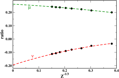
Figure 1: Right-hand-side ratios of Eqs. (6) and (7) (i.e. $\mu$ and $\nu$ values) computed for different noble-gas atoms up to $Z=290$. The extrapolation to $Z\rightarrow\infty$ was done using a parabolic fit as in Refs. EB09, ; ioni, ; PCSB, .

The values of the ratio on the right hand side of Eq. (6) for different noble-gas atoms, up to $Z=290$, are reported in Fig. 1 together with the extrapolation to $Z\rightarrow\infty$. We obtain $\mu^{MGE2}=0.262$, that is practically the same result as in Ref. EB09, .

In principle, Eq. (4) could be also used to obtain higher-order results. Nevertheless, such an approach is prone to large oscillations because the integral of $\epsilon_{x}^{exact}-\epsilon_{x}^{LDA}(1+\mu^{MGE2}s^{2})$ is small by construction, as it is that of $\epsilon_{x}^{LDA}s^{4}$, for $Z\rightarrow\infty$. Thus, in order to extend the modified gradient expansion to fourth order, we need to impose an additional constraint beyond the energy one. We do this by requiring that the modified gradient expansion not only reproduces the SCA asymptotic energy (which yields MGE2), but also gives a realistic SCA enhancement factor in the slowly-varying density limit. With this choice we also obtain to reduce the importance of high-density regions, which instead dominate the MGE2 behavior, since they are the ones that mostly contribute to the energy density, Thus, we can achieve a more balanced description of the whole slowly-varying regime (including low-density regions, which are rather important in real bulk solids). We recall that the enhancement factor is not an observable and is defined only up to a gauge transformation pb . Nevertheless, the enhancement factor $F_{x}^{exact}=\epsilon_{x}^{exact}/\epsilon_{x}^{LDA}$ of the conventional exact exchange energy density is well defined and has a clear physical meaning (i.e. it measures the interaction between an electron and the true exchange hole). Note also that the non-uniqueness problem is reduced in the slowly-varying density limit, where the exact exchange hole has a semilocal expansion Becke ; ernzerhof98 ; hole which becomes unique for the uniform electron gas. Thus, $F_{x}^{exact}$ can be safely used as a reference for our scope.

Following Eq. (6), we define an effective fourth-order coefficient (in the spirit of Eq. (3)) as

$$\nu^{MGE4}=\lim_{Z\rightarrow\infty}\frac{\int_{V}d\mathbf{r}\;(F_{x}^{exact}[Z]-F_{x}^{MGE2}[Z])}{\int_{V}d\mathbf{r}\;s[Z]^{4}}\ .$$ (7)

We remark that any fourth-order gradient expansion of the exchange energy diverges for atoms, because of the exponential decay of the density. Using the integration technique proposed in Eq. (7), we remove this difficulty and we focus on the slowly-varying density regime, that is the only one where a gradient expansion is well defined.

Finally, we highlight that the fourth-order gradient expansion of exchange depends, in general, on both the reduced gradient and the Laplacian. However, a Laplacian dependence is beyond the scope of this paper. Instead, using Eq. (7), we aim to extract an effective fourth-order coefficient in the spirit of Eq. (3).

The values of the ratio on the right hand side of Eq. (7) for different noble-gas atoms, up to $Z=290$, are reported in Fig. 1 together with the extrapolation to $Z\rightarrow\infty$. The behavior with $Z$ is regular, showing the physical meaningfulness of Eq. (7). Extrapolation to $Z\rightarrow\infty$ gives

$$\nu^{MGE4}=-0.195.$$ (8)

Note that this limit value is independent on the exact values used to define the boundaries of region $V$. Indeed, the same $\nu^{MGE4}$ is obtained using $-0.8\leq q\leq 0.8$ or $-1.2\leq q\leq 1.2$ (plots not reported).

The coefficient of Eq. (8), together with $\mu^{MGE2}$, define the modified fourth-order gradient expansion (MGE4), with the following enhancement factor

$$F_{x}^{MGE4}=1+\mu^{MGE2}s^{2}+\nu^{MGE4}s^{4}\ .$$ (9)

This reproduces, as close as possible, the conventional exact exchange enhancement factor in the slowly-varying density regime of non-relativistic large neutral atoms. Note that $\nu^{MGE4}$ is rather different from the fourth-order coefficient that is implicitly employed in APBE ($-(\mu^{MGE2})^{2}/\kappa=-0.084$).

The main features of the MGE4 can be seen in Fig. 2 where we plot, for the non-relativistic noble atom with 290 electrons and in the region $V$ defined before: the radial LDA exchange energy density, the reduced gradients $s$ and $q$, and the deviation, with respect to the exact conventional one, of the exchange enhancement factors of several gradient expansions. Here GE4 is the conventional fourth-order gradient expansion defined by the enhancement factor $F_{x}^{GE4}=1+10/81s^{2}+146/2025q^{2}-73/405qs^{2}+Ds^{4}$, where $D=0$ is the best numerical estimation for this parameter TPSS .

Figure 2: Radial LDA exchange energy density (top panel), reduced gradients $s$ and $q$ (middle panel), and (lower panel) the deviation, with respect to the exact conventional one, of the exchange enhancement factors of several gradient expansions, as functions of the distance $r$ from the nucleus, for the non-relativistic noble atom with 290 electrons.

We observe that:

$i)$ In the inner atomic core (i.e. for $r\lessapprox 1$), MGE2 is very accurate and, because both $s$ and $q$ are relatively small, the forth-order terms in gradient expansions are not much significant. Consequently, MGE4 is as accurate as MGE2. On the other hand, the GE2 and GE4 exchange enhancement factors are smaller, on average, than the exact one and they do not describe with high accuracy this energetical region. In fact, despite both $s$ and $q$ are not large in this region, only $q$ is very close to zero, while $s\approx 0.3$. Therefore, the conventional gradient expansions do not work very well in this regime. Note that the inner-core high-density region gives the main contribution to the exchange energy (99.3% of it).

$ii)$ In the outer atomic core (i.e. for $1\lessapprox r\lessapprox 4$), the reduced gradients $s$ and $q$ start to increase, but they are still smaller than 1, thus the density is still slowly-varying. This atomic region is not very important for the total exchange energy of atoms, but it is a model for solid-state problems (where the high-density limit is not common). While MGE2 fails in this region, the MGE4 and GE2 are very accurate.

II.1 Assessment of MGE4 for jellium cluster models

The MGE4 is accurate by construction for the slowly-varying density regime of large non-relativistic neutral atoms. To test it on a different model, we consider its performance for jellium clusters. These systems satisfy the uniform-electron-gas scaling scaling ($n_{\lambda}(\mathbf{r})=n(\lambda^{-1/3}\mathbf{r})$) and, in the limit of a large number of electrons, they are representative for solid-state systems.

In Fig. 3 we have plotted the relative error $\Delta E_{x}=(E_{x}^{exact}-E_{x}^{approx})/E_{x}^{LDA}$, computed over the volume ($V$ defined as in Eq. (7)), for jellium clusters of bulk parameter $r_{s}=4$ and up to $Z=2048$ electrons. The restriction of the intergal domain to the volume $V$ allows to remove the non-integrable region for the fourth-order terms (i.e. the tail of the density) and to consider solely the slowly-varying density region. The LDA, MGE2, and GE4 results are also reported in the figure.

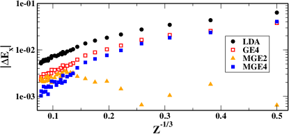
Figure 3: Relative exchange errors $|\Delta E_{x}|=|(E_{x}^{exact}-E_{x}^{approx})/E_{x}^{LDA}|$ for jellium clusters of bulk parameter $r_{s}=4$ and up to $Z=2048$.

It can be seen that MGE4 behaves similarly to GE4, which is derived from the slowly-varying density limit behavior. Actually, MGE4 gives even the best results for larger clusters. For these latter systems, MGE4 also outperforms MGE2, which is instead more accurate for the smallest clusters. To our knowledge, MGE4 is the only expansion which is realistic for atoms (that are characterized by the Thomas-Fermi scaling scaling $n_{\lambda}(\mathbf{r})=\lambda^{2}n(\lambda^{1/3}\mathbf{r})$) and jellium models (which are models for solid-state and are based on the uniform-electron-gas scaling scaling $n_{\lambda}(\mathbf{r})=n(\lambda^{-1/3}\mathbf{r})$).

II.2 Construction of a generalized gradient approximation functional based on MGE4

To demonstrate the practical utility of MGE4, we employ it to construct a simple generalized gradient approximation (GGA) functional named the Semiclassical GGA at fourth-order (SG4). Being based on MGE4, we expect that the SG4 functional performs well for both large atoms and solid-state systems; moreover, we will see that it is rather accurate also for ordinary chemistry.

The SG4 exchange enhancement factor takes the form

$$F_{x}^{SG4}=1+\kappa_{1}+\kappa_{2}-\frac{\kappa_{1}(1-\mu_{1}s^{2}/\kappa_{1})}{1-(\mu_{1}s^{2}/\kappa_{1})^{5}}-\frac{\kappa_{2}}{1+\mu_{2}s^{2}/\kappa_{2}},$$ (10)

where the condition $\kappa_{1}+\kappa_{2}=0.804$ is fixed from the Lieb-Oxford bound lieb81 , while $\mu_{1}+\mu_{2}=\mu^{MGE2}=0.26$ and $\kappa_{2}=-\mu_{2}^{2}/\nu^{MGE4}$ are imposed to recover MGE2 and MGE4, respectively. Note that in a Taylor expansion around $s=0$, the fourth term on the right hand side of Eq. (10) contributes only with $\mu_{1}s^{2}+\mathcal{O}(s^{10})$, whereas the MGE4 behavior is completely described by the last term. Such a simple splitting allows a better understanding of the physics behind the functional. It remains only one free parameter not fixed by the previous slowly-varying density conditions. We fix it to $\mu_{1}=0.042$ by fitting to the exchange ionization potential in the SCA limit (see Fig. 4).

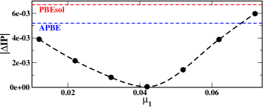
Figure 4: Absolute error (Ha) for the exchange ionization potential in the SCA limit as a function of the parameter $\mu_{1}$. The errors of the PBEsol and APBE functionals are also reported for reference.

In such a way, the SG4 exchange functional is completely constructed from the SCA model. Its enhancement factor is reported in Fig. 5. For small values of the reduced gradient $s$, it is close to the APBE one, since in this case MGE2 and MGE4 are very similar (they coincide in the limit of very small $s$ values). However, unlike APBE, the SG4 functional recovers MGE4 until $s\approx 0.6$. For larger values of the reduced gradient the SG4 enhancement factor is between the APBE and the PBEsol ones.

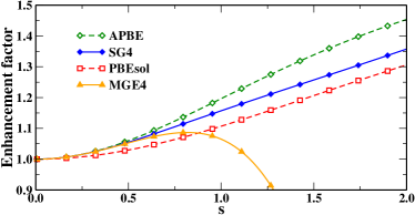
Figure 5: Enhancement factors of different functionals as functions of the reduced gradient $s$.

To complete the SG4 functional we need to complement it with a correlation functional. This must describe accurately the SCA correlation expansion $E_{c}\approx 0.02072Z\ln(Z)+BZ+\ldots$ (where $B=0.038$ is the best estimate for the first-order coefficient kc ), and recover the APBE correlation in the core of a large atom (i.e. for $r_{s}\rightarrow 0$ and $s\rightarrow 0$; note that, for exchange, SG4$\rightarrow$APBE in this limit). Hence, we consider the simple correlation energy per particle

$$\epsilon_{c}^{SG4}=\epsilon_{c}^{LDA}+\phi^{\alpha t^{3}}H(r_{s},\zeta,t),$$ (11)

where $t=|\nabla n|/(2k_{s}\phi n)$ is the reduced gradient for correlation pbe , with $k_{s}=(4k_{F}/\pi)^{1/2}$ being the Thomas-Fermi screening wave vector ($k_{F}=(3\pi^{2}n)^{1/3}$), $\phi={\left[\left(1+\zeta\right)^{2/3}+\left(1-\zeta\right)^{2/3}\right]}/2$ is a spin-scaling factor, $\zeta=(n_{\uparrow}-n_{\downarrow})/n$ is the relative spin polarization, and $H$ is a localized PBE-like gradient correction pbe ; tpssloc where we use

$$\beta=\beta_{0}+\sigma t(1-e^{-r_{s}^{2}})\ .$$ (12)

In order to recover the accurate LDA linear responseAPBE ; mukappa , we fix $\beta_{0}=3\mu^{MGE2}/\pi^{2}$. Moreover, we fix the parameter $\sigma=0.07$ fitting to jellium surface exchange-correlation energies js (in analogy to PBEsol PBEsol ) and $\alpha=0.8$ minimizing the information entropy function described in Ref. zint, . We recall that the spin-correction factor $\phi^{\alpha t^{3}}$ is always equal to one for spin-unpolarized systems (e.g. non magnetic solids), being important only in the rapidly-varying spin-dependent density regime (e.g. small atoms) zint .

Equations (10) and (11) define the SG4 exchange-correlation functional which satisfies, with no empirical parameters, many exact properties, including the constraints derived from the SCA theory.

III Results

In this section we present a general assessment of the performance of the SG4 functional for solid-state problems, which is the main topic of this work. For completeness, several atomic and molecular tests are also reported. Finally, we consider some application examples, to show the practical utility of MGE4 and the related SG4 functional in condensed-matter physics.

III.1 General assessment

At first, we consider a general assessment of the exchange only SG4 functional. This will allow a more direct evaluation of the importance of the MGE4 recovery. In Fig. 6 we show the relative errors $\Delta E_{x}=|E_{x}^{exact}-E_{x}^{approx}|/E_{x}^{LDA}$ for noble atoms (upper panel) and jellium clusters (lower panel), for several exchange functionals.

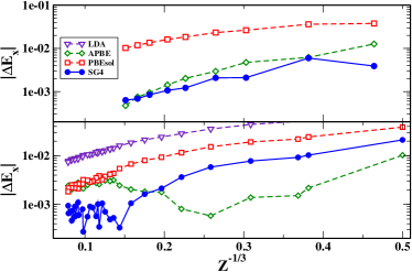
Figure 6: Relative exchange errors ($\Delta E_{x}=|E_{x}^{exact}-E_{x}^{approx}|/E_{x}^{LDA}$) for noble-gas atoms up to $Z=290$ electrons (upper panel) and for jellium clusters (lower panel) with $r_{s}=4$, up to $Z=2048$.

The PBEsol exchange, which is not based on the SCA theory, is not accurate for atoms PCSB , while APBE and SG4 are very accurate. This result is not highly surprising, since both these functionals are constructed to recover the SCA theory. Nevertheless, it is interesting to note that a good performance is obtained not only for very large atoms, but also for the moderately small ones. In the case of jellium clusters, APBE is the best for $Z<100$, while SG4 becomes more accurate for larger values of $Z$. According to the liquid-drop model theory of jellium spheres scaling , this means that it describes accurately the exchange quantum effects present in these systems.

Next, we discuss the performance of the full exchange-correlation SG4 functional for some basic solid-state tests. For completeness, several molecular tests are also reported.

Table 1: Mean absolute errors for equilibrium lattice constants and bulk moduli of a set of 29 bulk materials and for several chemistry tests [in detail, atomization energies of main-group molecules (G2/97) and transition metal complexes (TM10AE), metal-organic interfaces (SI12), bond lengths involving H atoms (MGHBL9) and not involving H atoms (MGNHBL11), interaction energies of hydrogen bond and dipole-dipole complexes (HB6+DI6), interaction energies of dihydrogen bond complexes (DHB23)]. The best (worst) results of each line are in boldface (underlined).

	APBE	PBE	SG4	PBEsol	WC
Lattice constants (mÅ)
simple metals	34.1	31.4	41.7	55.6	58.4
transition metals	63.7	44.9	23.9	25.6	23.7
semiconductors	102.3	85.3	21.0	32.7	31.5
ionic solids	95.6	76.0	20.8	20.0	18.8
insulators	34.0	27.8	8.0	8.5	8.0
total MAE	66.0	53.0	24.9	31.0	30.7
LC20	70.3	55.9	23.1	34.0	31.8
bulk moduli (GPa)
simple metals	1.3	1.1	0.7	0.2	0.54
transition metals	26.3	21.2	20.0	20.2	18.9
semiconductors	18.7	16.9	5.8	8.2	8.0
ionic solids	9.6	8.5	6.2	3.9	4.8
insulators	18.6	15.3	4.9	6.2	6.1
total MAE	14.8	12.4	7.9	8.2	8.0
cohesive energies (eV)
simple metals	0.09	0.05	0.21	0.15	0.13
transition metals	0.32	0.21	0.39	0.62	0.51
semiconductors	0.29	0.13	0.09	0.28	0.20
ionic solids	0.19	0.14	0.20	0.07	0.06
insulators	0.12	0.16	0.36	0.57	0.47
total MAE	0.21	0.14	0.24	0.33	0.27
Molecular tests (kcal/mol ; mÅ)
G2/97	8.9	14.8	15.7	37.7	27.6
TM10AE	11.1	13.0	11.9	18.3	15.8
SI12	5.9	3.7	2.6	3.8	3.3
MGHBL9	10.0	11.5	10.3	14.5	13.9
MGNHBL11	9.2	7.6	3.7	5.2	6.1
HB6+DI6	0.4	0.4	0.5	1.3	0.9
DHB23	0.8	1.0	1.1	1.8	1.6

In Table 1 we show the results of SG4 calculations for the lattice constants, bulk moduli, and cohesive energies of a set of 29 bulk solids (see Section V). Our benchmark set for lattice constants includes, as a subset, the LC20 benchmark set of Refs. coads, ; SCAN, , which is also reported in Table 1. The comparison is done with APBE APBE , that is the other non-empirical XC functional based on the SCA theory, as well as with the PBEsol PBEsol , PBE pbe , and Wu-Cohen (WC) wc functionals, which are among the most popular GGAs for solids (another popular solid-state functional is the AM05 am05 ; am05_2 ; am05_3 (not reported), which performs similarly to PBEsol and WC).

It can be seen that SG4 works remarkably well for solids. It outperforms APBE (and PBE) and is often even better than the state-of-the-art GGA for solids PBEsol and WC. The comparison of the SG4 results for lattice constants and bulk moduli with the APBE ones shows the relevance of MGE4 for solid-state systems. We highlight that the SG4 result for the LC20 test (MAE=23.1 mÅ) also competes with the ones of the best meta-GGAs for solids. From literature, we found indeed the following MAEs for the LC20 test set: TPSS = 43 mÅcoads , revTPSS = 32 mÅcoads , SCAN = 16 mÅSCAN . This is a remarkable performance of the SG4 functional for the equilibrium lattice constants of bulk solids, suggesting that the MGE4 gradient expansion can also be a useful tool for further meta-GGA development.

The results for the cohesive energies display a quite different trend. Actually, this property involves a difference between results from bulk and atomic calculations. Thus, the best results are found for the PBE functional, which provides the best error cancellation (note that PBE is the best neither for solid-state nor for atoms). The SG4 functional performs overall similarly as the APBE one, being slightly penalized by the need to include small atoms’ calculations. Nevertheless, SG4 definitely outperforms PBEsol, which yields a quite poor description of all atoms.

Cohesive energy results can be rationalized even better looking at the outcome of several molecular tests. These tests are also useful to obtain a more comprehensive assessment of the performance of the functionals, even though we recall that the focus of the present paper is on solid-state properties. Moreover, the comparison of SG4 with PBEsol provides a hint of the relevance of the SCA theory underlying the SG4 construction.

Inspection of the lowest panel of Table 1 shows that SG4 is quite accurate for molecular tests. It is comparable with PBE for atomization and non-covalent energies (within chemical accuracy), and very accurate for geometry and interaction energies at interfaces. The latter results are especially interesting, since these tests require a delicate balance between the description of different density regimes mukappa , which is important for broad applicability at the GGA level PBEint ; mukappa ; htbs . In particular, the molecular bond lengths in the MGNHBL11 test (that do not imply bonds with hydrogen atoms) are best described by semilocal functionals with low non-locality mukappa (e.g. PBEsol), while the ones in the MGHBL9 test require a large amount of non-locality (APBE works at best). SG4 appears to be able to capture well both situations and yields a total mean absolute error (MAE) for geometry of 6.7 mÅ, better than both APBE (9.5 mÅ) and PBE (9.4 mÅ).

III.2 Surface and monovacancy formation energies

Table 2: (111) surface energies (J/m²) and monovacancy formation energies (eV) in several simple and transition metals. Mean absolute errors (MAE) are reported in the last line. Values in best agreement with experiments q2d ; singhmiller09 ; luo12 ; vitos ; delczeg09 ; ehrhart ; schaefer87 ; deboer88 are in boldface.

Metal	PBEsol	SG4	Exp.
Surface energies (J/m2)
Al	0.96	1.06	1.14
Ca	0.52	0.54	0.50
Sr	0.40	0.41	0.42
Cu	1.61	1.67	1.79
Pt	1.83	1.89	2.49
Rh	2.45	2.51	2.70
Au	0.98	1.01	1.50
Pd	1.69	1.72	2.00
MAE	0.27	0.23
Monovacancy energy (eV)
Cu	1.25	1.35	1.28
Ni	1.73	1.83	1.79
Pd	1.49	1.59	1.85
Ir	1.88	2.04	1.97
Au	0.65	0.78	0.89
Pt	1.02	1.15	1.35
MAE	0.19	0.13

In Table 2 we report the surface energies of three simple metals and five transition metals, as well as the monovacancy formation energies in several transition metals. These tests involve a comparison between bulk energies in a delocalized electronic system (metal) and the energy of the quite localized surface/vacancy. Thus, they may be the ideal playground for the SG4 functional which shows a good performance for bulk, being simultaneously quite accurate also for confined systems thanks to the underlying SCA theory.

Indeed, SG4 performs remarkably well for both problems, yielding MAEs of 0.23 J/m² and 0.13 eV, which compare favorably with those of PBEsol (0.27 J/m² and 0.19 eV). WC is close to PBEsol but slightly worse (MAEs are 0.29 J/m² and 0.22 eV); PBE and APBE are systematically worse than PBEsol and are not reported. Notably, the improvement is also systematic, since SG4 is always closer to the experimental values than PBEsol, with the only exception of Ca and Cu for surface and monovacacy formation energies, respectively.

III.3 Structure of boehmite and diaspore crystals

In Table 3 we list the structural parameters, as defined in Fig. 7, computed for the boehmite and diaspore crystals.

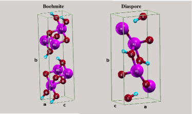
Figure 7: Structural parameters of boehmite and diaspore crystals.

Table 3: Lattice parameters ($a$, $b$, $c$) and various atomic distances for the boehmite and diaspore crystals. All data are in Å. The reference data are taken from Refs. hill79, ; corbato85, . The best result for each line is highlighted in bold.

	PBEsol	SG4	Exp.
Boehmite
a	2.868	2.863	2.868
b	11.839	11.858	12.234
c	3.714	3.713	3.692
Al-O	1.911	1.909	1.907
OH	1.027	1.019	0.970
H$\cdots$O	1.545	1.565	1.738
Diaspore
a	4.360	4.362	4.401
b	9.411	9.399	9.425
c	2.848	2.842	2.845
Al-O	1.917	1.915	1.915
OH	1.039	1.031	0.989
H$\cdots$O	1.524	1.535	1.676

These systems consist of layers of aluminum hydroxides bound together by hydrogen bonds. We recall that layered solids are becoming increasingly important in materials science applications, thanks to their anisotropic behavior. However, an accurate description of the equilibrium structure of these systems requires the ability to describe both covalent and non-covalent bonds in the bulk with similar accuracy. This is a quite difficult task for GGAs demichelis10 .

In general, the PBEsol functional is among the best GGAs for boehmite and diaspore demichelis10 . It describes with good accuracy the covalent bonds, but it suffers of some limitations in the description of the non-covalent ones. The SG4 functional preserves the good features of PBEsol and provides, in addition, small but important and systematic improvements for hydrogen bonds.

III.4 Ice lattice mismatch problem

The ice lattice mismatch problem is a popular problem in solid-state physics feibelman08 ; fang13 . It involves the calculation of the lattice constant $a$ of ice Ih and of the lattice constant $b$ of $\beta$-AgI, which are used to define the lattice mismatch

$$f=\frac{2(b-a)}{b+a}\ .$$ (13)

The lattice mismatch $f$ is an important quantity in many applications, since it determines the growth rate of ice on a $\beta$-AgI surface (for example, $\beta$-AgI is used as seed crystal to produce artificial rainfall). However, the computational determination of the lattice mismatch is a quite hard task, since it involves the simultaneous calculation of the lattice constants of two materials with quite different electronic properties. For this reason its calculation is a challenge for semilocal density functionals feibelman08 ; fang13 .

In Table 4 we report the computed lattice constants and the corresponding lattice mismatch, as obtained from several functionals. In this case we also report PBE results, since for this problem PBE is one of the best GGAs, performing better than PBEsol.

Table 4: Calculated lattice constants (Å) for ice Ih and $\beta$-AgI as well as the corresponding lattice mismatch. Experimental data are taken from Ref. feibelman08, . The best result for each line is highlighted in bold.

	PBE	PBEsol	SG4	Exp.
a (ice Ih)	4.42	4.29	4.33	4.50
b ($\beta$-AgI)	4.68	4.56	4.57	4.59
mismatch	5.7%	6.1%	5.4%	2.2%

Indeed, we see that PBE yields quite good results for the lattice constant of both materials, showing errors below 0.1 Å in both cases. However, because the errors for ice Ih and $\beta$-AgI lattice constants have opposite signs, the final lattice mismatch is computed rather inaccurately. On the other hand, PBEsol performs well for $\beta$-AgI, but yields a much larger error for ice Ih. Thus, the resulting lattice mismatch is definitely overestimated. A better balance in the performance is seen instead in the SG4 case. This functional is in fact the best for $\beta$-AgI and between PBE and PBEsol for ice Ih. Hence, it finally yields a lattice mismatch of 5.4%. This value is still too large with respect to the experimental one (2.2%), but improves with respect to the other GGAs.

IV Summary and concluding remarks

In this paper we have used the SCA theory to introduce a modified fourth-order gradient expansion (MGE4), which is accurate for atoms and solid-state systems. The MGE4 includes and extends the well-known MGE2. The extension over MGE2 is obtained by using, in the gradient expansion construction, an additional constraint, beyond the energy one, which provides an improved description of slowly-varying regions of different materials. To implement the new constraint, an integration over slowly-varying density regions was introduced in order to reduce computational noise and avoid the divergence of fourth order terms in rapidly-varying density regions.

To exploit the good features of MGE4 we have used it as a base to construct a simple GGA functional, named SG4. This functional is free of parameters fitted on real systems and satisfies several exact properties, including those relevant for the SCA model, the Lieb-Oxford bound, the LDA linear response behavior, and the rapidly-varying as well as the high-density limits of correlation. The SG4 functional performs well for a broad range of problems in solid-state physics, still preserving, thanks to the SCA underlying theory, a reasonable performance also for molecular tests. Due to this eclectic character, the SG4 functional is particularly promising for problems involving multiple electronic structure features, such as surface energies, vacancies, non-covalent interactions in bulk solids, and interfaces.

The results of the present work highlight, through the power of MGE4 for different problems, the importance of the underlying SCA model as a reference system in DFT also for solid-state systems. This was the primary goal of the present work, since the relevance of the SCA model system was often overlooked in the literature and the utility of this model has been often considered to be limited to the atomic and molecular framework.

To conclude we recall that gradient expansions are basic tools for the contruction of non-empirical DFT functionals, even beyond the semilocal XC level TPSS ; Becke ; ernzerhof98 ; final1 ; final2 ; final3 ; final4 . Thus, in the future, further studies may focus on the use of MGE4 to construct and optimize highly accurate functionals of different ranks, beyond the simple SG4 that we have presented here mainly to illustrate the practical utility of the SCA theory.

V Computational details

All atomic calculations used to derive the MGE4 expansion have been performed using the Engel code engel with the exact exchange functional. Further tests of the MGE4 on jellium clusters have been carried out employing accurate LDA Kohn-Sham densities tao08 .

The SG4 functional has been tested on different datasets, including

• Atomization and interaction energies: atomization energies of small molecules (G2/97 g2_1 ; g2_2 ), atomization energies of small transition metal complexes (TM10AE furche06 ; zint ; zvint ), small gold-organic interfaces (SI12 hpbeint ).

• Structural properties: bond lengths involving H atoms (MGHBL9 mgbl19 ), bond lengths not involving H atoms (MGNHBL11 mgbl19 ) bonds.

• Non-covalent interactions: interaction energies of hydrogen-bond and dipole-dipole complexes (HB6+DI6 zhao05 ) as well as of dihydrogen bond complexes (DHB23 dihydro ).

• Solid-state tests: Equilibrium lattice constants and bulk moduli of 29 solids, including Al, Ca, K, Li, Na, Sr, Ba (simple metals); Ag, Cu, Pd, Rh, V, Pt, Ni (transition metals); LiCl, LiF, MgO, NaCl, NaF (ionic solids); AlN, BN, BP, C (insulators); GaAs, GaP, GaN, Si, SiC, Ge (semiconductors). Reference data to construct this set were taken from Refs. coads, ; harl10, ; schimka11, ; csonka09, ; janthon14, .

All calculations for molecular systems have been performed with the TURBOMOLE program package turbomole ; turbo_rev , using a def2-TZVPP basis set basis1 ; basis2 . Calculations concerning solid-state tests have been performed with the VASP program vasp , using PBE-PAW pseudopotentials. We remark that the use of the same pseudopotential for all the functionals may lead to inaccuracies in the final results. Nevertheless, the use of PAW core potentials ensures good transferability for multiple functionals am05_3 ; paier05 , since the core-valence interaction is recalculated for each functional. Indeed, test calculations employing different variants of the PAW potentials (GGA-PAW) have shown that the estimated convergence level of our calculations is about 1 mÅ for lattice constants, 0.5 GPa for bulk moduli, and 0.01 eV for cohesive energies. All Brillouin zone integrations were performed on $\Gamma$-centered symmetry-reduced Monkhorst-Pack $k$-point meshes, using the tetrahedron method with Blöchl corrections. For all the calculations a $24\times 24\times 24$ $k$-mesh grid was applied and the plane-wave cutoff was chosen to be 30% larger than maximum cutoff defined for the pseudopotential of each considered atom. The bulk modulus was obtained using the Murnaghan equation of state. The cohesive energy, defined as the energy per atom needed to atomize the crystal, is calculated for each functional from the energies of the crystal at its equilibrium volume and the spin-polarized symmetry-broken solutions of the constituent atoms. To generate symmetry breaking solutions, atoms were placed in a large orthorhombic box with dimensions $13\times 14\times 15$ ų.

Calculations for the examples reported in subsections III.2, III.3, and III.4 have been performed using the same computational setups as in Refs. luo12, ; delczeg09, ; demichelis10, ; feibelman08, .

Acknowledgments. We thank Prof. K. Burke for useful discussions and TURBOMOLE GmbH for providing the TURBOMOLE program. E. Fabiano acknowledges a partial funding of this work from a CentraleSupélec visiting professorship.

References

- (1) P. Hohenberg and W. Kohn, Phys. Rev. 136, B864 (1964).
- (2) W. Kohn and L. J. Sham, Phys. Rev. , A1133 (1965).
- (3) J. F. Dobson, G. Vignale, and M. P. Das, Electronic Density Functional Theory, Springer (1998).
- (4) G. E. Scuseria and V. N. Staroverov, Progress in the development of exchange-correlation functionals, Chapter 24 in: Theory and Applications of Computational Chemistry: The First 40 Years (A Volume of Technical and Historical Perspectives), edited by C. E. Dykstra, G. Frenking, K. S. Kim, and G. E. Scuseria, Elsevier, Amsterdam (2005).
- (5) D. Rappoport, N. R. M. Crawford, F. Furche, and K. Burke, Approximate Density Functionals: Which Should I Choose?, in Encyclopedia of Inorganic Chemistry,ohn Wiley & Sons (2009), DOI: 10.1002/0470862106.ia615.
- (6) B. Civalleri, D. Presti, R. Dovesi, and A. Savin, On choosing the best density functional approximation, in Chemical Modelling : Applications and Theory Volume 9, The Royal Society of Chemistry (2012).
- (7) J. P. Perdew, A. Ruzsinszky, G. I. Csonka, O. A. Vydrov, G. E. Scuseria, L. A. Constantin, X. Zhou, and K. Burke, Phys. Rev. Lett. , 136406 (2008); ibid. , 039902 (E); ibid. , 239702 (2008).
- (8) Y. Zhao and D. G. Truhlar, J. Chem. Phys. 128, 184109 (2008).
- (9) R. Peverati, Y. Zhao and D. G. Truhlar, J. Phys. Chem. Lett. 2, 1991 (2011)
- (10) E. Fabiano, L. A. Constantin, and F. Della Sala, Phys. Rev. B 82, 113104 (2010).
- (11) A. Vela, J. C. Pacheco-Kato, J. L. Gázquez, J. M. del Campo, and S. B. Trickey, J. Chem. Phys.136, 144115 (2012).
- (12) A. Vela, V. Medel, and S. B. Trickey, J. Chem. Phys. 130, 244103 (2009).
- (13) L. S. Pedroza, A. J. R. da Silva, and K. Capelle, Phys. Rev. B 79, 201106(R) (2009).
- (14) A. Ruzsinszky, G. I. Csonka, and G. E. Scuseria, J. Chem. Theory Comput. , 763 (2009).
- (15) E. Fabiano, L. A. Constantin, A. Terentjevs, F. Della Sala, P. Cortona, Theor. Chem. Acc. 134, 139 (2015).
- (16) J. Tao, J. P. Perdew, V. N. Staroverov, and G. E. Scuseria, Phys. Rev. Lett. , 146401 (2003).
- (17) J.P. Perdew, A. Ruzsinszky, G. I. Csonka, L. A. Constantin, and J. Sun, Phys. Rev. Lett. , 026403 (2009); (Erratum) Phys. Rev. Lett. , 179902(E) (2011).
- (18) L.A. Constantin, E. Fabiano, F. Della Sala, J. Chem. Theory Comput. , 2256 (2013).
- (19) J. Sun, R. Haunschild, B. Xiao, I.W. Bulik, G. E. Scuseria, and J. P. Perdew, J. Chem. Phys. , 044113 (2013).
- (20) J. M. del Campo, J. L. Gázquez, S. B. Trickey , A. Vela, Chem. Phys. Lett. 543, 179 (2012).
- (21) J. Sun, A. Ruzsinszky, and J.P. Perdew, Phys. Rev. Lett. , 036402 (2015).
- (22) R. Peverati and D.G. Truhlar, J. Phys. Chem. Lett. 3, 117 (2012)
- (23) L. H. Thomas, Proc. Cambridge Phil. Soc. , 542 (1926).
- (24) E. Fermi, Rend. Accad. Naz. Lincei , 602 (1927).
- (25) J. M. C. Scott, Philos. Mag. , 859 (1952).
- (26) J. Schwinger, Phys. Rev. A , 1827 (1980).
- (27) J. Schwinger, Phys. Rev. A , 2353 (1981).
- (28) B.-G. Englert and J. Schwinger, Phys. Rev. A , 2339 (1984).
- (29) B.-G. Englert and J. Schwinger, Phys. Rev. A , 26 (1985).
- (30) P. Elliott and K. Burke, Can. J. Chem. , 1485 (2009).
- (31) P. Elliott, D. Lee, A. Cangi, and K. Burke, Phys. Rev. Lett. , 256406 (2008).
- (32) D. Lee, L. A. Constantin, J. P. Perdew, and K. Burke, J. Chem. Phys. , 034107 (2009).
- (33) J. P. Perdew, L. A. Constantin, E. Sagvolden, and K. Burke, Phys. Rev. Lett. , 223002 (2006).
- (34) L. A. Constantin, E. Fabiano, S. Laricchia, and F. Della Sala, Phys. Rev. Lett. , 186406 (2011).
- (35) E. Fabiano, L. A. Constantin, P. Cortona, and F. Della Sala, J. Chem. Theory Comput. 11, 122 (2015).
- (36) L. A. Constantin, J. C. Snyder, J. P. Perdew, and K. Burke, J. Chem. Phys. , 241103 (2010).
- (37) E. H. Lieb and S. Oxford, Int. J. Quantum Chem. 19, 427 (1981).
- (38) L. A. Constantin, A. Terentjevs, F. Della Sala, and E. Fabiano, Phys. Rev. B , 041120(R) (2015).
- (39) G. K. H. Madsen, Phys. Rev. B 75, 195108 (2007)
- (40) Z. Wu and R. E. Cohen, Phys. Rev. B 73, 235116 (2006).
- (41) Y. Zhao and D.G. Truhlar 78, 197101 (2008)
- (42) F. Della Sala, E. Fabiano, L. A. Constantin, Phys. Rev. B 91, 035126 (2015).
- (43) J. P. Perdew, V.N. Staroverov, J. Tao, and G. E. Scuseria, Phys. Rev. A , 052513 (2008).
- (44) A. D. Becke, J. Chem. Phys. , 1040 (1996).
- (45) M. Ernzerhof and J. P. Perdew, J. Chem. Phys. , 3313 (1998).
- (46) L. A. Constantin, E. Fabiano, and F. Della Sala, Phys. Rev. B 88, 125112 (2013).
- (47) E. Fabiano and L. A. Constantin, Phys. Rev. A , 012511 (2013).
- (48) K. Burke, A. Cancio, T. Gould, and S. Pittalis, arXiv:1409.4834 [cond-mat.mtrl-sci].
- (49) J. P. Perdew, K. Burke, and M. Ernzerhof, Phys. Rev. Lett. , 3865 (1996).
- (50) L. A. Constantin, E. Fabiano, and F. Della Sala, Phys. Rev. B , 035130 (2012).
- (51) E. Fabiano, L. A. Constantin, and F. Della Sala, J. Chem. Theory Comput. 7, 3548 (2011).
- (52) L. A. Constantin, L. Chiodo, E. Fabiano, I. Bodrenko, F. Della Sala, Phys. Rev. B 84, 045126 (2011).
- (53) L. A. Constantin, E. Fabiano, and F. Della Sala, Phys. Rev. B , 233103 (2011).
- (54) R. Armiento and A. E. Mattsson, Phys. Rev. B 72, 085108 (2005).
- (55) A. E. Mattsson and R. Armiento, Phys. Rev. B 79, 155101 (2009).
- (56) A. E. Mattsson, R. Armiento, J. Paier, G. Kresse, J. M. Wills, and T. R. Mattsson, J. Chem. Phys. 128, 084714 (2008).
- (57) J. Paier, R. Hirschl, M. Marsman, and G. Kresse, J. Chem. Phys. 122, 234102 (2005).
- (58) J. Sun, M. Marsman, G. I. Csonka, A. Ruzsinszky, P. Hao, Y.-S. Kim, G. Kresse, and J. P. Perdew, Phys. Rev. B 84, 035117 (2011).
- (59) P. Haas, F. Tran, P. Blaha, and K. Schwarz, Phys Rev. B 83, 205117 (2011).
- (60) L. Chiodo, L. A. Constantin, E. Fabiano, and F. Della Sala, Phys. Rev. Lett. 108, 126402 (2012).
- (61) N. E. Singh-Miller and N. Marzari, Phys. Rev. B 80, 235407 (2009)
- (62) S. Luo, Y. Zhao, and D. G. Truhlar, J. Phys. Chem. Lett. 3, 2975 (2012).
- (63) L. Vitos, A. V. Ruban, H. L. Skriver, and J. Kollar, Surf. Sci. 411, 186 (1998).
- (64) L. Delczeg, E. K. Delczeg-Czirjak, B. Johansson, and L. Vitos, Phys. Rev. B 80, 205121 (2009).
- (65) P. Ehrhart, P. Jung, H. Schultz, and H. Ullmaier, Atomic Defects in Metals, Landolt-Börnstein, New Series, Group III vol 25, Springer (1991).;
- (66) H.-E. Schaefer, Phys. Stat. Sol. (a) 102, 47 (1987).
- (67) F. R. de Boer, R. Boom, W. C. M. Mattens, A. R. Miedema, and A. K. Niessen, Cohesion in Metals, Vol. 1, North-Holland, Amsterdam (1988).
- (68) R. Hill, J. Phys. Chem. Miner. 5, 179 (1979).
- (69) C. E. Corbato, R. T. Tettenhorst, and G. G. Christoph, Clays Clay Miner. 33, 71 (1985).
- (70) R. Demichelis, B. Civalleri, P. D’Arco, and R. Dovesi, Int. J. Quant. Chem. 110, 2260 (2010).
- (71) P. J. Feibelman, Phys. Chem. Chem. Phys. 10, 4688 (2008).
- (72) Y. Fang, B. Xiao, J. Tao, J. Sun, and J. P. Perdew, Phys. Rev. B 87, 214101 (2013).
- (73) M. M. Odashima and K. Capelle, Phys. Rev. A 79, 062515 (2009).
- (74) R. Hanunschild, M. M. Odashima, G. E. Scuseria, J. P. Perdew, and K. Capelle, J. Chem. Phys. 136, 184102 (2012).
- (75) G. Vignale and W. Kohn, Phys. Rev. Lett. 77, 2037 (1996).
- (76) J. F. Dobson and B. P. Dinte, Phys. Rev. Lett. 76, 1780 (1996).
- (77) E. Engel, in A Primer in Density Functional Theory, Eds. C. Fiolhais, F. Nogueira, M. A. L. Marques, Springer Berlin, pp 56–122 (2003).
- (78) J. Tao, J. P. Perdew, L. M. Almeida, C. Fiolhais, and S. Kümmel, Phys. Rev. B 77, 245107 (2008).
- (79) L. A. Curtiss, K. Raghavachari, P. C. Redfern, and J. A. Pople, J. Chem. Phys. 106, 1063 (1997).
- (80) R. Haunschild and W. Klopper, J. Chem. Phys. 136, 164102 (2012).
- (81) F. Furche and J. P. Perdew, J. Chem. Phys. 124, 044103 (2006).
- (82) L. A. Constantin, E. Fabiano, and F. Della Sala, J. Chem. Phys. 137, 194105 (2012).
- (83) E. Fabiano, L. A. Constantin, and F. Della Sala, Int. J. Quantum Chem. 13, 6670 (2012)
- (84) Y. Zhao and D. G. Truhlar, J. Chem. Phys. 125, 194101 (2006).
- (85) Y. Zhao and D. G. Truhlar, J. Chem. Theory Comput. 1, 415 (2005).
- (86) E. Fabiano, L. A. Constantin, and F. Della Sala, J. Chem. Theory Comput. 10, 3151 (2014).
- (87) J. Harl, L. Schimka, and G. Kresse, Phys. Rev. B 81, 115126 (2010).
- (88) L. Schimka, J. Harl, and G. Kresse, J. Chem. Phys. 134, 024116 (2011).
- (89) G. I. Csonka, J. P. Perdew, A. Ruzsinszky, P. H. T. Philipsen, S. Lebègue, J. Paier, O. A. Vydrov, and J. G. Ángyán, Phys. Rev. B 79, 55107 (2009).
- (90) P. Janthon, S. Luo, S. M. Kozlov, F. Viñes, J. Limtrakul, D. G. Truhlar, and F. Illas, J. Chem. Theory Comput. 10, 38323839 (2014).
- (91) TURBOMOLE, V6.3; TURBOMOLE GmbH: Karlsruhe, Germany, 2011. Available from http://www.turbomole.com (accessed May 2015).
- (92) F. Furche, R. Ahlrichs, C. Hättig, W. Klopper, M. Sierka, and F. Weigend, WIREs Comput. Mol. Sci. 4, 91 (2014).
- (93) F. Weigend, F. Furche, and R. Ahlrichs, J. Chem. Phys. 119, 1275312763 (2003).
- (94) F. Weigend and R. Ahlrichs, Phys. Chem. Chem. Phys. 7, 3297 (2005).
- (95) G. Kresse and J. Furthmuller, Phys. Rev. B 54, 11169 (1996).