One-dimensional hydrodynamic model generating a turbulent cascade

Abstract

As a minimal mathematical model generating cascade analogous to that of the Navier-Stokes turbulence in the inertial range, we propose a one-dimensional partial-differential-equation model that conserves the integral of the squared vorticity analogue (enstrophy) in the inviscid case. With a large-scale random forcing and small viscosity, we find numerically that the model exhibits the enstrophy cascade, the broad energy spectrum with a sizable correction to the dimensional-analysis prediction, peculiar intermittency and self-similarity in the dynamical system structure.

I Introduction

One way to tackle the problem of fluid turbulence is to study its model with a drastically reduced degrees of freedom. These models are made in mostly phenomenological ways to qualitatively have a few, selected aspects of turbulence. Celebrated models include the Burgers’ equation burg and the shell models Bi , which are certainly more amenable to analytical and numerical studies. Another family tree of these models stems from the Constantin-Lax-Majda (CLM) model clm . We find a turbulent solution of this model family for the first time and discuss its relevance to two-dimensional Navier-Stokes turbulence.

The CLM model was introduced to study the problem of putative finite-time blowup of the incompressible Euler equation in three dimensions, that is, whether or not the vorticity becomes infinite in a finite time starting from a smooth initial condition mb . The CLM model is a one-dimensional partial differential equation which models the three-dimensional (3D) inviscid vorticity equation. The velocity gradient in the vortex-stretching term is modeled as the Hilbert transform of the scalar vorticity to incorporate the Biot-Savart nonlocality. But the model omits the advection term. Significantly, the model has an explicit analytic solution blowing up in a finite time. The natural question was soon addressed: does the (hypo-) viscous effect, let us say adding the Laplacian (or various orders thereof) of the model vorticity, prevent a solution from blowing up? Unfortunately the answer was no scho ; saka ; The vorticity invariably blows up in finite time however large order of the Laplacian is added. This is in contrast to the existence of 3D Navier-Stokes (NS) solutions with the Laplacian of order larger than $5/4$ rs .

This indicates that the vortex stretching in the CLM equation is modeled somewhat excessively. Given that the viscosity is not enough to suppress the blowup, what if the omitted advection term is retained in the CLM model? This was first considered by De Gregorio dg1 ; dg2 and it is numerically shown that there exists a unique smooth solution to the CLM equation with the advection term globally in time oswn , implying that the advection term is able to prevent the blowup, although a rigorous proof is unavailable as yet. Subsequently, in order to study balance between the advection and stretching terms for the existence of solutions, the generalized Constantin-Lax-Majda-De Gregorio (gCLMG) model, $\partial_{t}\omega+au\partial_{x}\omega=\omega\partial_{x}u$, was introduced in oswn . Here $a\in\mathbb{R}$ is a parameter discussed below, $\omega(x,t)$ denotes the model vorticity and the model velocity $u(x,t)$ is expressed in terms of the vorticity as $u=-(-\partial_{xx})^{-1/2}\omega$ and $\partial_{x}u=H(\omega)$ which is the Hilbert transform of $\omega$. The parameters $a=0$ and $a=1$ correspond to the CLM model and the CLM model with advection term, respectively. Note also that, for general $a$, the Galilean invariance is lost. Mathematically, the short-time existence of solutions of the gCLMG equation is proven for all $a$ oswn , while it is conjectured that there exists some critical value, $a_{c}\sim 0.6$, above which a solution exists globally in time oswdcds .

Here is a twist: negative $a$ can be considered oswn at the expense of the analogy of the gCLMG model to the 3D vorticity equation. Instead, we gain the conservation law: for $a<0$, it is shown easily that $\int|\omega(x,t)|^{-a}dx$ is conserved oswn . For $a=-1$, the blowup of $\partial_{x}\omega$ is proven rigorously ccf , while for $a=-2$ only numerical evidence for the blowup is available.

With these mathematical facts about the gCLMG model, we address the following natural question: does a viscous gCLMG model work as a physical model of turbulence? It is thus reasonable to consider the following forced viscous gCLMG model:

$$\partial_{t}\omega+au\partial_{x}\omega=\omega\partial_{x}u+\nu\partial_{xx}\omega+f,$$ (1)

where $\nu$ is the model kinematic viscosity and $f(x,t)$ represents an external force. For $a=1$, albeit the similarity to the 3D vorticity equation, our numerical result shows that the model’s energy concentrates on the forcing scale and the inertial range (IR) is not developed at all. This indicates that the model is inadequate for NS turbulence in the IR. The reason for this inadequacy can be that the model admits no conserved quantity such as the energy. On the other hand, for $a=-2$, the (model) enstrophy becomes the conservative quantity of the inviscid gCLMG model. Such quadratic conservation law is an essential element of NS turbulence as stressed, e.g., in f . In this respect, the gCLMG model is akin to the 2D NS equation rather than the 3D vorticity equation. Therefore, our aim in this paper is to investigate whether Eq.(1) with $a=-2$ serves as a model of the enstrophy-cascade turbulence of the two-dimensional (2D) incompressible NS equations. Among features of the enstrophy-cascade turbulence km ; t ; g ; b , we focus on similarities and differences of the energy spectrum, in particular, the Kraichnan’s logarithmic correction k71 ; lk72 to the Kraichnan-Leith-Batchelor (KLB) energy spectrum, $k^{-3}$ k67 ; l68 ; b69 , and of the structure function of the vorticity. We also try to describe the gCLMG turbulence from a dynamical system point of view.

II Numerical simulation of the model

We numerically simulate the gCLMG equation (1) for $a=-2$ in a periodic interval of length $2\pi$ with a standard dealiased spectral method by assuming null vorticity Fourier mode of the zero wavenumber using the fourth order Runge-Kutta scheme and the same filtering of the round-off noise as oswn . To achieve a statistically steady state, the large-scale forcing $f(x,t)$ is set to be random: its Fourier coefficient $\hat{f}(k,t)$ is non zero only for the forcing wavenumbers $k=\pm 1$, whose real and imaginary parts are set to Gaussian, delta-correlated-in-time and independent random variables with zero mean and variance, $\sigma_{f}^{2}$. Specifically, with keeping $\sigma_{f}=1.0\times 10^{-2}$ (the average enstrophy-input rate is thus $2\sigma_{f}^{2}=2.0\times 10^{-4}$), we vary the kinematic viscosity as $\nu=\nu_{0}\times 4^{-m}~{}(m=0,1,2)$ with $\nu_{0}=2.5\times 10^{-5}$. The corresponding time step, $\Delta t$, and the number of grid points, $N$, are $(\Delta t,N)=(2.5\times 10^{-4}\times 2^{-m},2^{13+m})$.

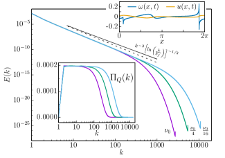
Figure 1: Top inset: a typical snapshot of the vorticity with pulse structures and the velocity of the randomly forced gCLMG equation. Main figure: the time-averaged energy spectra, $E(k)$, of the forced gCLMG equation for three values of the viscosity. The dashed line is Eq.(3) for the inertial range. Bottom inset: the corresponding time-averaged enstrophy fluxes, $\Pi_{Q}(k)$. The plateau value is equal to the average enstrophy input rate.

In the top inset of Fig.1, we show an example of the vorticity and velocity from the middle viscosity case. It is seen that the gCLMG turbulent state is characterized by several pulses of the vorticity, which move randomly and sometimes merge and emerge. The energy spectra, $E(k)=\sum_{k\leq|k^{\prime}|<k+1}|\hat{u}(k^{\prime},t)|^{2}/2$ ($\hat{u}(k^{\prime},t)$ is the velocity Fourier coefficient), for the three cases are plotted in Fig.1. It exhibits the IR and dissipation range. Indeed, as shown in the bottom inset of Fig.1, the enstrophy flux, $\Pi_{Q}(k,t)$, in the Fourier space of the gCLMG equation defflux has a plateau which extends to larger wavenumbers as we diminish the kinematic viscosity. The enstrophy flux is defined as $\Pi_{Q}(k,t)=\sum_{\ell(\ell\geq k)}\sum_{k^{\prime}~{}(|k^{\prime}|=\ell)}\sum_{p,q~{}(p+q=k^{\prime})}{\rm Im}[\hat{\omega}^{*}(k^{\prime},t)(aq-p)\hat{u}(p,t)\hat{u}(q,t)]$, where $\hat{\omega}(k^{\prime},t)$ is the vorticity Fourier coefficient and ^∗ denotes complex conjugate. Here we regard the plateau region as the IR of the gCLMG turbulence. Having obtained evidence of the enstrophy cascade in the forced gCLMG turbulence, however, we observe that the energy spectrum $E(k)$ in the IR has a visible correction to the KLB law, $E(k)\propto\beta^{2/3}k^{-3}$, where $\beta$ is the average enstrophy dissipation rate. This law is the simplest dimensional-argument result on the enstrophy-cascade spectrum in the IR k67 ; l68 ; b69 . Moreover, the gCLMG spectrum deviates also from the Kraichnan’s prediction with the logarithmic correction about the 2D NS enstrophy-cascade turbulence, $k^{-3}[\ln(k/k_{f})]^{-1/3}$ k71 ; lk72 , where the forcing wavenumber is $k_{f}=1$ here. If we fit $E(k)$ with a pure power law, $k^{-\gamma}$, without the logarithmic correction, the exponent is close to $\gamma=3.5$. Nevertheless, we observe that dependence of $E(k)$ on $\beta$ is consistent with the KLB law from collapse of $E(k)\beta^{-2/3}$ onto a single curve in the inertial range for various enstrophy dissipation rates (figure not shown). This indicates that the scaling behavior of the model is determined by the enstrophy cascade. The scaling of the energy spectrum will be examined in terms of the vorticity structure function.

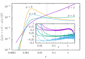
Figure 2: Even order ($p=2,4,6,8$) structure functions of the vorticity for the smallest viscosity case. The vertical dashed line corresponds to $r=2\pi/200$. The inertial range is here estimated as $2\pi/200\leq r\leq\pi$ from the bottom inset of Fig.1 in which the plateau extends from $2\leq k\leq 200$. Inset: logarithmic local slopes of the structure functions ($p=2,4,6$ from top to bottom) for the three viscosity cases. Oscillations tend to be reduced as we increase the number of statistical samples (the slope for $p=8$ is not shown because they are so large). The vertical dashed lines correspond to the respective smallest scales in the IR.

Now we move to the $p$-th order structure function of the vorticity, $S_{p}(r)=\langle(\delta_{r}\omega)^{p}\rangle$, where $\delta_{r}\omega=\omega(x+r,t)-\omega(x,t)$ and $\langle\cdot\rangle$ denotes space-time average. In Fig.2, $S_{p}(r)$ are shown in the log-log coordinates. It appears that $S_{2}(r)$ is close to $r^{0.5}$, which is consistent with $E(k)\propto k^{-3.5}$. However the logarithmic local slope, $[\ln S_{2}(r+\Delta r)-\ln S_{2}(r)]/[\ln(r+\Delta r)-\ln r]$ ($\Delta r$ being the grid size), does not converge to a unique constant value in the IR as we decrease $\nu$. One possibility is that the power-law exponent of $S_{2}(r)$ in the IR depends on $\nu$ (similar dependence was found for the velocity structure function of the 2D enstrophy-cascade turbulence cg ). Another possibility is that the dominant part of $S_{2}(r)$ is not a pure power law but with a correction. For the fourth order, it is seen that $S_{4}(r)$ is nearly constant in the IR. Now let us assume that the even-order structure function is a pure power law with exponent $\zeta_{2n}$ to the leading order, i.e., $S_{2n}(r)\propto r^{\zeta_{2n}}$. Then the relation $\zeta_{2}>\zeta_{4}$, as indicated in Fig.2, implies that the vorticity cannot be bounded (see Sec. 8.4 of Ref.f ). With a given enstrophy input, $\omega$ of the gCLMG turbulence can be infinite for $\nu\to 0$ as we will see later. This is in contrast to the velocity of the incompressible fluids. Conversely, if we consider that $\omega$ should be bounded, then $S_{2n}(r)$ is not pure power law but with a correction. We now have two scenarios: (i) the pure power law, $E(k)\propto k^{-3.5}$ and $S_{2}(r)\propto r^{0.5}$, leading to infinite vorticity and (ii) the power law with a correction, $E(k)\propto k^{-3}\times$(non-power-law correction) and $S_{2}(r)\propto$(non-power law part), with bounded vorticity. We will later present evidence for (ii) while the infinite vorticity as $\nu\to 0$ is indicated simultaneously.

For higher orders, we observe that $S_{6}(r)$ and $S_{8}(r)$ have a peak in the dissipative range and that they are decreasing functions in the IR. The peaks are due to the biggest pulse of the vorticity (the rightmost one in the top inset of Fig.1) as expected. The scale of the peak, $r\simeq 0.002$, coincides with the typical width of the biggest pulse. About the decreasing behavior in the IR, it is unlikely to be an artefact caused by the peak since the decreasing region extends for smaller $\nu$ as seen in the bottom inset of Fig.2. Then do $S_{6}(r)$ and $S_{8}(r)$ have negative scaling exponents in the IR, as discussed for the 2D enstrophy-cascade turbulence ey ? Our answer is yes, but with non power-law corrections since the logarithmic slopes (here shown only for $S_{6}(r)$) are not satisfactorily flat. The negative exponents are consistent with the singular behavior of the vorticity (see f ). We conclude that $E(k)$ and $S_{p}(r)$ of the gCLMG turbulence in the IR are not described by a pure power law but with certain corrections and that $S_{p}(r)$’s behavior indicates a singularity of the vorticity.

Now we compare the above results of the gCLMG turbulence with those obtained for the 2D NS enstrophy-cascade turbulence (henceforth 2D turbulence). We limit ourselves here to experimental and numerical results of the 2D turbulence having only the enstrophy-cascade IR as a statistically steady state (not a decaying state). Concerning the energy spectrum, the difference from the KLB $k^{-3}$ scaling is more measurable in the gCLMG turbulence than in the 2D turbulence. The spectrum of the latter is occasionally fitted with the power law $k^{-3.3}$ g ; b ; cee ; cg ; rae . Regarding the vorticity structure functions of the 2D turbulence, the result obtained in the laboratory experiment pct showed that those of even orders up to $10$ in the IR have power-law exponents indistinguishable from zero. This is consistent with the theoretical results beyond dimensional analysis of the 2D turbulence fl ; ey . We note that in pct no indication of $\zeta_{2}>\zeta_{4}$ was observed, assuming that the structure function in the IR is a power-law function. Numerical results of the 2D turbulence showed that $S_{2}(r)$ is logarithmic without a power law and that $S_{4}(r)$ is a decreasing function vl , however. Switching to the velocity, we observe that both the even-order velocity structure functions and the even-order moments of the second-degree increments of the velocity fra of the gCLMG turbulence are not power-law functions in the IR as indicated by their logarithmic local slopes without plateau. This is in contrast with the 2D turbulence bclvv ; cg . Therefore, the gCLMG turbulence obeys distinct statistics from the 2D turbulence despite the analogous enstrophy cascade. However both have statistics with non power-law type corrections in common. Further details will be studied with a stationary solution of Eq.(1) as follows.

III Stationary solution

Surprisingly, the forced gCLMG equation has a stable stationary solution whose energy spectrum is indistinguishable to that of the gCLMG turbulence in the IR, as shown in Fig.3. We find it incidentally when we change the random forcing to a deterministic and stationary one, $f(x,t)=C_{0}\sin x$, in order to study dependence of the statistics on the large-scale forcing. Thus it demonstrates the striking forcing dependence. We here fix the forcing amplitude $C_{0}=-0.1$ and vary $\nu$ as $10^{-4}\times 4^{-m}~{}(m=0,1,\ldots,5)$. We use the same spectral method and time stepping as before with the corresponding time step $\Delta t=2.5\times 10^{-4}\times 2^{-m}$ and the number of grid points $N=2^{13+m}$. The stationary solution has one vorticity pulse as depicted in the right inset of Fig.3, which is likely to converge to a singular function (infinite vorticity) as $\nu\to 0$ (analogously nonsmooth vorticity has been observed in the 2D stationary Kolmogorov flow for small $\nu$ o96 ). Its peak value and width are numerically found to scale with $\nu^{-0.2}$ and $\nu^{0.6}$, leading to the enstrophy dissipation rate independent on $\nu$.

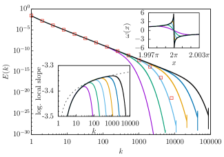
Figure 3: The energy spectra of the stationary solutions to the gCLMG equation with the deterministic forcing for various $\nu$’s. The squares represent data (multiplied by $20$) of the randomly forced case with $\nu_{0}/8$ shown in Fig.1. Left inset: the logarithmic local slopes of the energy spectra and Eq.(2) as the dashed line. Right inset: the vorticity pulses of the stationary solutions.

The identity of the energy spectrum of the stationary solution to that of the gCLMG turbulence in the IR implies that the functional form of the turbulent $E(k)$ can be studied with the stationary solution. In the left inset of Fig.3, we plot the plateau-less logarithmic local slope of $E(k)$, demonstrating no pure power law in the IR. We then make the following ansatz in the IR,

$$\frac{\ln\frac{E(k+\Delta k)}{E(k)}}{\ln\frac{k+\Delta k}{k}}\simeq k\frac{d}{dk}\ln E(k)=-c_{0}-c_{1}\left[\ln\mbox{$\left(\frac{k}{k_{f}}\right)$}\right]^{\delta},$$ (2)

although small discrepancy among $\nu$’s are present (but not visible in the bottom inset of Fig.3). For $\delta\neq-1$, integration of Eq.(2) leads to the expression of the energy spectrum,

$$E(k)\propto k^{-c_{0}}\exp\left\{-c_{2}\left[\ln\mbox{$\left(\frac{k}{k_{f}}\right)$}\right]^{\theta}\right\},$$ (3)

where $c_{2}=c_{1}/(1+\delta)$ and $\theta=1+\delta$. Here we fix the first parameter as $c_{0}=3$ in view of the enstrophy cascade and our previous observation of $E(k)$’s dependence on the enstrophy dissipation rate. The rest of the parameters are estimated as $c_{1}=0.442$ and $\delta=-0.138$ by fitting Eq.(2) in the range $20\leq k\leq 1000$, resulting in $c_{2}=0.513$ and $\theta=0.862$. So far Eqs.(2-3) are empirical (but $\theta=-1$ case can be obtained with the incomplete self-similarity bc ). The log-corrected spectrum of the form $E(k)\propto k^{-3}\ln^{\alpha}(k/k_{f})$, corresponding to $c_{1}=-\alpha$ and $\delta=-1$, does not yield a better fit however we adjust $\alpha$, implying that this type of the correction is not suitable for the gCLMG turbulence.

 

 

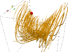
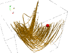
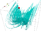
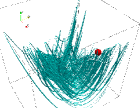
Figure 4: Self-similarity of the phase-space orbits of ${\rm Im}[\hat{\omega}(k,t)]$ of the randomly forced gCLMG turbulence ($\nu=\nu_{0}/4$ case) for $k=4,8,16$ (top) and $k=32,64,128$ (bottom) as $(x,y,z)$ variables from two angles of view. The point corresponds to the stationary solution with the same enstrophy and viscosity.

To see further relation of the stationary solution to the gCLMG turbulence from a dynamical system point of view, we plot in Fig.4 an orbit of the randomly forced case in the three dimensional subspace of the phase space, which is defined as $({\rm Im}[\hat{\omega}(k_{1},t)]/\Omega(k_{1})-1,\,{\rm Im}[\hat{\omega}(k_{2},t)]/\Omega(k_{2})-1,\,{\rm Im}[\hat{\omega}(k_{3},t)]/\Omega(k_{3})-1)$. Here ${\rm Im}[\hat{\omega}(k,t)]$ and $\Omega(k)$ are the imaginary part of the vorticity Fourier coefficient of the randomly forced gCLMG equation and the stationary solution, respectively. We take wavenumber triplet $(k_{1},k_{2},k_{3})$ as $(4,8,16)$ and $(32,64,128)$ which are in the IR except for $128$. Hence we look at the orbit scaled with the stationary solution from the two ranges of scales. We observe that the orbit is within a thin surface with the stationary solution located on one edge of this attracting set. Significantly, the orbits in the two scale ranges are similar. With this self-similarity of the orbit, modeling of the gCLMG turbulence with a few degrees of freedom is conceivable.

IV Summary

We numerically studied the gCLMG equation Eq.(1) with $a=-2$ with a large-scale forcing. The random forcing generates the turbulent state analogous to the 2D NS enstrophy-cascade turbulence due to existence of the inviscid quadratic invariant, the enstrophy. The deterministic forcing yields the stable stationary solution which is spectrum-wise relevant to the gCLMG turbulence. The statistical laws of the gCLMG turbulence, such as the measurable corrections to the KLB law, are quantitatively different from the 2D turbulence. However, qualitatively, statistics not characterized by simple power laws are common. Therefore we expect that the simpler gCLMG model provides insight in theoretical study of these subtle statistics, which are not captured by dimensional analysis. Currently, we failed to substantiate our expectation although the stationary solution should facilitate analytical study. Another remarkable aspect of the gCLMG solutions is the strong indication of infinite vorticity with a finite enstrophy dissipation rate as $\nu\to 0$, possibly an inheritance from the CLM model. This implies that the gCLMG model is an interesting testing ground for investigating relation between singularity and turbulence statistics. However, we note that the finite-limit of the enstrophy dissipation rate is not shared with the 2D enstrophy-cascade turbulence (see, e.g.,d1 ; d2 ). For different negative $a$’s in Eq.(1), we found that the similar results to the $a=-2$ case holds, which will be reported elsewhere.

References

- (1) J. Bec and K. Khanin, Phys. Rep., 447, 1–66 (2007).
- (2) L. Biferale, Ann. Rev. Fluid Mech., 35, 441-468 (2003).
- (3) P. Constantin, P.D. Lax and A. Majda, Comm. Pure App. Math., 28, 715–724 (1985).
- (4) A.J. Majda and A.L. Bertozzi, Vorticity and Incompressible flow, Cambridge Univ. Press (2001).
- (5) S. Schochet, Comm. Pure App. Math., 39, 531–537 (1986).
- (6) T. Sakajo, Nonlinearity, 16, 1319–1328 (2003).
- (7) H.A. Rose and P.-L. Sulem, J. de Physique, 39, 441–484 (1978).
- (8) S. De Gregorio, J. Stat. Phys., 59, 1251–1263 (1990).
- (9) S. De Gregorio, Math. Methods App. Sci., 19, 1233–1255 (1996).
- (10) H. Okamoto, T. Sakajo and M. Wunsch, Nonlinearity, 21, 2447–2461 (2008).
- (11) H. Okamoto, T. Sakajo and M. Wunsch, Disc. Conti. Dyn. Sys., 34, 3155–3170 (2014).
- (12) A. Córdoba, D. Córdoba and M.A. Fontelos, Ann. Math., 162, 1377–1389 (2005).
- (13) U. Frisch, Turbulence, Cambridge Univ. Press (1996).
- (14) R.H. Kraichnan and D. Montgomery, Rep. Prog. Phys., 43, 547–619 (1980).
- (15) P. Tabeling, Phys. Rep., 362, 1–62 (2002).
- (16) H. Kellay and W.I. Goldburg, Rep. Prog. Phys., 65, 845–894 (2002).
- (17) G. Boffetta and R.E. Ecke, Ann. Rev. Fluid Mech., 44, 427–451 (2012).
- (18) R.H. Kraichnan, J. Fluid Mech., 47, 525–535 (1971).
- (19) C. Leith and R.H. Kraichnan, J. Atmos. Sci., 29, 1041–1058 (1972).
- (20) R.H. Kraichnan, Phys. Fluids, 10, 1417–1423 (1967).
- (21) C. Leith, Phys. Fluids, 11, 671–673 (1968).
- (22) G.K. Batchelor, Phys. Fluids, 12, II-233–239 (1969).
- (23) R.T. Cerbus and W.I. Goldburg, Phys. Fluids, 25, 105111 (2013).
- (24) S. Chen, R.E. Ecke, G.L. Eyink, X. Wang and Z. Xiao, Phys. Rev. Lett., 91, 214501 (2003).
- (25) M.K. Rivera, H. Aluie and R.E. Ecke, Phys. Fluids, 26, 055105 (2014).
- (26) J. Paret, M.-C. Jullien and P. Tabeling, Phys.Rev.Lett., 83, 3418–3421 (1999).
- (27) G. Falkovich and V. Lebedev, Phys. Rev. E, 49, R1800–R1803 (1994).
- (28) G.L. Eyink, Physica D, 91, 97–142 (1996).
- (29) A. Vallgren and E. Lindborg, J. Fluid Mech., 671 168–183 (2011).
- (30) E. Falcon, S.G. Roux and B. Audit, EPL, 90, 50007 (2010).
- (31) L. Biferale, M. Cencini, A. Lanotte, D. Vergni and A. Vulpiani, Phys. Rev. Lett., 87, 124501 (2001).
- (32) H. Okamoto, J. Dyn. Diff. Eq., 8, 203–220 (1996).
- (33) G.I. Barenblatt and A.J. Chorin, Proc. Natl. Acad. Sci. USA, 93, 6749–6752 (1996).
- (34) C.V. Tran and D.G. Dritschel, J. Fluid Mech., 559, 107–116 (2006).
- (35) D.G. Dritschel, C.V. Tran and R.K. Scott, J. Fluid Mech., 591, 379–391 (2007).