Model independence of the measurement of the $\mathrm{e}^{+}\mathrm{e^{-}\rightarrow\mathrm{ZH}}$ cross section using $\mathrm{\mathrm{\mathrm{Z\rightarrow\mu^{+}\mu^{-}}}}$ and $\mathrm{Z\rightarrow\mathrm{e^{+}\mathrm{e^{-}}}}$ at the ILC

Abstract

The model independent measurement of the absolute cross section ($\sigma_{\mathrm{ZH}}$) of the Higgsstrahlung process $\mathrm{e^{+}e^{-}\rightarrow ZH}$ is an unique measurement at the ILC indispensable for measuring the Higgs couplings and their deviations from the Standard Model in order to identify new physics models. The performance in measuring $\sigma_{\mathrm{ZH}}$ using events in which the Higgs boson recoils against a Z boson which decays into a pair of muons or electrons has been demonstrated based on full simulation of the ILD detector for three center of mass energies $\sqrt{s}$ = 250, 350, and 500 GeV, and two beam polarizations $\left(P\mathrm{e^{-}},P\mathrm{e^{+}}\right)$ =($-$80%, +30%) and (+80%, $-$30%). This paper demonstrates in detail that the analysis which achieved these results are model independent to the sub-percent level. Data selection methods are designed to optimize the precisions of $\sigma_{\mathrm{ZH}}$ and at the same time minimize the bias on the measured $\sigma_{\mathrm{ZH}}$ due to discrepancy in signal efficiencies among Higgs decay modes. Under conservative assumptions which take into account unknown Higgs decay modes, the relative bias on $\sigma_{\mathrm{ZH}}$ is shown to be smaller than 0.2% for all center-of-mass energies, which is five times below even the smallest $\sigma_{\mathrm{ZH}}$ statistical uncertainties expected from the leptonic recoil measurements in a full 20 years ILC physics program.

High Energy Accelerator Research Organization (KEK), Tsukuba 305-0801, Japan

1 INTRODUCTION

It is one of the most important missions of high energy particle physics to uncover the physics behind electroweak symmetry breaking (EWSB). The discovery of the Standard Model (SM)-like Higgs boson at the Large Hadron Collider (LHC) in 2012 [1, 2] proved the basic idea of the SM that the vacuum filled with the Higgs condensate broke the electroweak symmetry. The SM assumes one doublet of complex scalar fields for the Higgs sector. However, apart from the fact that it is the simplest, there is no reason to prefer the Higgs sector in the SM over any other model that is consistent with experiments. Moreover, the SM does not explain why the Higgs field became condensed in vacuum. To answer this question, we need physics beyond the SM (“BSM”) which necessarily alters the properties of the Higgs boson. Each new physics model predicts its own size and pattern of the deviations of Higgs boson properties from their SM predictions. In order to discriminate these new physics models, we need to measure with high precision as many types of couplings as possible and as model independently as possible. Because the deviations predicted by most new physics models are typically no larger than a few percent, the coupling measurements must achieve a precision of 1% or better for a statistically significant measurement. This level of sensitivity is available only in the clean experimental environment of lepton colliders.

The International Linear Collider (ILC) [3] is a proposed $\mathrm{e^{+}e^{-}}$ collider covering center-of-mass energy range of 200 to 500 GeV, with expandability to 1 TeV. Among the most important aspects of its physics program [4] are the measurements of Higgs couplings with unprecedented precision so as to find their deviations from the SM and match their deviation pattern with predictions of various new physics models.

Most of the Higgs boson measurements at the LHC are measurements of cross section times branching ratio (BR). This is also true at the ILC with one important exception, the measurement of the absolute size of an inclusive Higgs production cross section by applying the recoil technique to the Higgsstrahlung process $\mathrm{e^{+}e^{-}\rightarrow ZH}$. The recoil technique involves measuring only the momenta of the decay products of the Z boson which recoils against the Higgs boson, and hence in principle is independent of the Higgs decay mode. The measurement of this cross section $\sigma_{\mathrm{ZH}}$ is indispensable for extracting the branching ratios, the Higgs total width, and couplings from cross section times branching ratio measurements. The recoil technique, which is only possible at a lepton collider owing to the well-known initial state, is applicable even if the Higgs boson decays invisibly and hence allows us to determine $\sigma_{\mathrm{ZH}}$ in a completely model independent way, as will be shown in this paper. Especially high precision measurements of $\sigma_{\mathrm{ZH}}$ and $M_{\mathrm{H}}$ are possible by applying the recoil technique to Higgsstrahlung events where the Z boson decays to a pair of electrons or muons, which profits from excellent tracking momentum resolution and relatively low background levels. Furthermore, in this channel model independence for the measurement of $\sigma_{\mathrm{ZH}}$ can be demonstrated in practice.

A study reported in [6] evaluates the performance of measuring $\sigma_{\mathrm{ZH}}$ and the Higgs boson mass $M_{\mathrm{H}}$ using Higgsstrahlung events with leptonic Z boson decays $\mathrm{e^{+}e^{-}\rightarrow ZH\rightarrow\mathrm{\mathit{\mathrm{l^{+}l^{-}}}H}}$ ($\mathrm{l}$ = e or $\mu$) for three center-of-mass energies (250, 350, and 500 GeV), as well as two beam polarizations $\left(P\mathrm{e}^{-},P\mathrm{e}^{+}\right)$ =($-$80%, +30%) and (+80%, $-$30%), which will be denoted as $\mathrm{e_{L}^{-}}\mathrm{e_{R}^{+}}$ and $\mathrm{e_{R}^{-}}\mathrm{e_{L}^{+}}$, respectively. The results in [6] will be scaled to the “H20” program [5], which designates that during a 20 year period, a total of 2000, 200, and 4000 $\mathrm{fb^{-1}}$ will be accumulated at $\sqrt{s}$= 250, 350, and 500 GeV, respectively. This paper reports a study which demonstrates that the measurement of $\sigma_{\mathrm{ZH}}$ in [6] is model independent to a level well below the expected statistical precision from the full ILC physics program. The methods of signal selection and background rejection studied here are those used for producing the results in [6].

This paper is structured as follows: Section 2 explains the recoil measurement; Section 3 introduces the simulation tools, the ILC detector concept, and the signal and physics background processes; Section 4 presents the methods of data selection optimized for this analysis; Section 5 describes the efforts to minimize Higgs decay mode bias and evaluates the bias on the measured $\sigma_{\mathrm{ZH}}$; Finally Section 6 summarizes the analysis and concludes the paper.

2 HIGGS BOSON MEASUREMENTS USING THE RECOIL TECHNIQUE

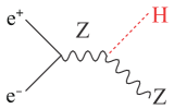
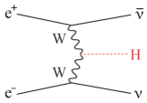
The major Higgs production processes at the ILC are Higgsstrahlung and WW fusion, whose lowest order Feynman diagrams are illustrated in Figure 1, along with the ZZ fusion process which has a significantly smaller cross section than the other two processes at ILC center-of-mass energies. Figure 2 shows the production cross sections as a function of $\sqrt{s}$, assuming a Higgs boson mass of 125 GeV.

Figure 1: The lowest order Feynman diagrams of the three major Higgs production processes at the ILC: (left) Higgsstrahlung process $\mathrm{e^{+}e^{-}\rightarrow ZH}$ , (center) WW fusion process $\mathrm{e^{+}e^{-}\rightarrow\nu\overline{\nu}H}$ , and (right) ZZ fusion process $\mathrm{e^{+}e^{-}\rightarrow e^{+}e^{-}H}$.

Figure 2: The Higgs production cross section as a function of $\sqrt{s}$ assuming $M_{\mathrm{H}}$=125 GeV for the following Higgs production processes: Higgsstrahlung (solid), WW fusion (dashed), and ZZ fusion (dotted). (Figure taken from [3].)

The Higgsstrahlung process with a Z boson decaying into a pair of electrons or muons: $\mathrm{e^{+}e^{-}\rightarrow ZH\rightarrow\mathit{\mathrm{l^{+}l^{-}}}H}$ ( $\mathrm{l}$ = e or $\mu$) will be hereafter referred to as $\mathrm{e^{+}e^{-}H}$ and $\mathrm{\mu{}^{+}\mathit{\mu}^{-}H}$, respectively. The leptonic recoil technique is based on the Z boson identification by the invariant mass of the dilepton system being consistent with the Z boson mass, and the reconstruction of the mass of the rest of the final-state system recoiling against the Z boson ($M_{\mathrm{rec}}$), corresponding to the Higgs boson mass, which is calculated as

$$M_{\mathrm{rec}}=\left(\sqrt{s}-E_{\mathrm{l^{+}l^{-}}}\right)^{2}-\left|\overrightarrow{p}_{\mathrm{l^{+}l^{-}}}\right|^{2}\>,$$ (1)

where $E_{\mathrm{l^{+}l^{-}}}\equiv E_{\mathrm{l^{+}}}+E_{\mathrm{l^{-}}}$ and $\overrightarrow{p}_{\mathrm{l^{+}l^{-}}}\equiv\overrightarrow{p}_{\mathrm{l}^{+}}+\overrightarrow{p}_{\mathrm{l}^{-}}$ are the energy and momentum of the lepton pair from Z boson decay. The $M_{\mathrm{rec}}$ calculated using Equation 1 is expected to form a peak corresponding to Higgs boson production. From the location of the $M_{\mathrm{rec}}$ peak and the area beneath it the Higgs boson mass and the signal yield can be extracted. The production cross section ($\sigma_{\mathrm{ZH}}$) can be obtained as :

$$\sigma_{\mathrm{ZH}}=\frac{N_{S}}{BR\mathrm{\left(\mathrm{Z\rightarrow\mathrm{l^{+}l^{-}}}\right)\varepsilon}_{S}L}\>,$$ (2)

where $N_{S}$ is the number of selected signal events, $\varepsilon_{\mathrm{S}}$ is the efficiency of signal event selection, and $L$ is the total integrated luminosity. In principle, $\varepsilon_{\mathrm{S}}$ and hence $\sigma_{\mathrm{ZH}}$ are independent of how the Higgs boson decays, since only the leptons from the Z decay need to be measured in the recoil technique. In practice, however, this is not completely guaranteed since there is a possibility of confusion between the leptons from the Z boson decay and those from the Higgs boson decay. Thus this paper aims to demonstrate that the signal efficiency is indeed independent of assumptions regarding Higgs boson decay, based on the Higgs recoil analysis given in detail in in [6].

3 ANALYSIS FRAMEWORK, DETECTOR SIMULATION, AND EVENT GENERATION

3.1 Analysis framework

This study used the simulation and reconstruction tools contained in the software package ILCSoft v01-16 [8]. All parameters of the incoming beams are simulated with the GUINEA-PIG package [9] and the beam spectrum, including beamstrahlung and ISR, are explicitly taken into consideration based on the parameters in the TDR. The beam crossing angle of 14 mrad in the current ILC design is taken into account. The $\mathrm{\mu{}^{+}\mathit{\mu}^{-}H}$, $\mathrm{e^{+}e^{-}H}$, and SM background samples (see Section 3.3 for details) are generated using the WHIZARD 1.95 [10] event generator. The input mass of the Higgs boson is 125 GeV, and its SM decay branching ratios are assumed [11]. The model for the parton shower and hadronization is taken from PYTHIA 6.4 [12]. The generated events are passed through the ILD [13] simulation performed with the MOKKA [14] software package based on GEANT4 [15]. Event reconstruction is performed using the Marlin [16] framework. The PandoraPFA [17] algorithm is used for calorimeter clustering and the analysis of track and calorimeter information based on the particle flow approach.

3.2 The ILD concept

The International Large Detector (ILD) concept [13] is one of the two detectors being designed for the ILC. It features a hybrid tracking system with excellent momentum resolution. The jet energy resolution is expected to be better than 3% for jets with energies $\geq$ 100 GeV, thanks to its highly granular calorimeters optimized for Particle Flow reconstruction [17]. This section describes the ILD sub-detectors important for this study.

The vertex detector (VTX), consisting of three double layers of extremely fine Si pixel sensors with the innermost radius at 15 mm, measures particle tracks with a typical spatial resolution of 2.8 $\mathrm{\mu m}$. The hybrid tracking system consists of a time projection chamber (TPC) which provides up to 224 points per track, excellent spatial resolution of better than 100 $\mathrm{\mu m}$, and $dE/dx$ - based particle identification, as well as Si-strip sensors placed in the barrel region both inside and outside the TPC and in the endcap region outside the TPC in order to further improve track momentum resolution. The tracking system measures charged particle momenta to a precision of $\frac{\delta p_{t}}{p_{t}^{2}}=2\times 10^{-5}$$\mathrm{\;GeV^{-1}}$. Outside of the tracking system sits the ECAL, a Si-W sampling electromagnetic calorimeter with an inner radius of 1.8 m, finely segmented $5\times 5$ $\mathrm{mm^{2}}$ transverse cell size and 30 longitudinal layers equivalent to 24 radiation lengths. The HCAL, a steel-scintillator type hadronic calorimeter which surrounds the ECAL, has an outer radius of 3.4 m, $3\times 3$ $\mathrm{cm^{2}}$ transverse tiles, and 48 longitudinal layers corresponding to 5.9 interaction lengths. Radiation hard calorimeters for monitoring the luminosity and quality of the colliding beams are installed in the forward region. The tracking system and calorimeters are placed inside a superconducting solenoid which provides a magnetic field of 3.5 T. An iron yoke outside the solenoid coil returns the magnetic flux, and is instrumented with scintillator-based muon detectors.

3.3 Signal and background processes

The Higgsstrahlung signal is selected by identifying a pair of prompt, isolated, and oppositely charged muons or electrons with well-measurable momentum whose invariant mass $M_{\mathrm{l^{+}l^{-}}}$ ($\mathrm{l}$=$\mathrm{e}$ or $\mu$) is close to the Z boson mass ($M_{\mathrm{Z}}$). The $\mathrm{\mu{}^{+}\mathit{\mu}^{-}H}$ and $\mathrm{e^{+}e^{-}H}$ channels are analyzed independently and then statistically combined. Figure 3 shows the Feynman diagrams of the dominant 4-fermion and 2-fermion processes. Table 1 gives the cross sections of signal and major background processes assuming $M_{\mathrm{H}}$=125 GeV. For each process, all SM tree-level diagrams are included by WHIZARD. These processes are grouped as follows from the perspective of finding leptons in the final state:

• $\mathrm{l^{+}l^{-}}\mathrm{H}$ ($\mathrm{l}$=$\mathrm{e}$ or $\mu$) : The Higgsstrahlung signal process with Z decaying to $\mathrm{l^{+}l^{-}}$. The $\mathrm{e^{+}e^{-}H}$ channel contains an admixture of the ZZ fusion process, which is removed at the early stages of the analysis.

• 2-fermion leptonic (2f_l): final states consisting of a charged lepton pair or a neutrino pair. The intermediate states are Z or $\gamma^{*}$.

• 4-fermion leptonic (4f_l): final states of 4 leptons consisting of mainly processes through ZZ and WW intermediate states. Those events containing a pair of electrons or muons are a background of the $\mathrm{\mu{}^{+}\mathit{\mu}^{-}H}$ and $\mathrm{e^{+}e^{-}H}$ channels, respectively.

• 4-fermion semileptonic (4f_sl): final states of a pair of charged leptons and a pair of quarks, consisting of mainly processes through ZZ and WW intermediate states. In the former case, one Z boson decays to a pair of charged leptons or neutrinos, and the other to quarks. In the latter case, one W boson decays to a charged lepton and a neutrino of the same flavor and the other to quarks.

• 4(2)-fermion hadronic (4(2)f_h): final states of 4 (2) quarks. Since the probability of finding isolated leptons is very small for these final states, these events are removed almost completely at the lepton identification stage (see Section 4.1).

The analysis in this paper and [6] are conducted for the center-of-mass energies 250, 350, and 500 GeV, and two beam polarization $\mathrm{e_{L}^{-}e_{R}^{+}}$ and $\mathrm{e_{R}^{-}e_{L}^{+}}$. From Table 1, it can be seen that the signal cross sections for $\mathrm{e_{R}^{-}e_{L}^{+}}$ is smaller by a factor of 1.5 with respect to $\mathrm{e_{L}^{-}e_{R}^{+}}$, whereas the total background is suppressed by a factor of 2 and some individual background processes are suppressed by a factor of up to 10. The methods and performance of signal selection and background rejection are presented in Section 4.

The Monte Carlo (MC) samples are generated for the cases in which $\left(P\mathrm{e^{-}},P\mathrm{e^{+}}\right)$ =($-$100%, +100%) and (+100%, $-$100%). The standard samples used in [6] are generated for signal and background processes with the statistics as shown in Table 1, and the events are and normalized to the assumed integrated luminosities, cross sections, and polarizations. Another type of signal sample is generated with high statistics of more than 40k for each major SM Higgs decay mode, mainly for the purpose of the model independence study in this paper.

Figure 3: The Feynman diagrams contributing to the major background processes for the Higgs recoil analysis in the $\mathrm{\mu{}^{+}\mathit{\mu}^{-}H}$ channel: 2f_l background with $\mu\mu$ in the final state and an ISR photon (left), 4f_sl background with ZZ as intermediate state (center), 4f_l background with WW as intermediate state (right).

$\sqrt{s}$ = 250 GeV	cross	section	$N_{\mathrm{Gen}}$
polarization	left	right	left	right
$\mathrm{\mu{}^{+}\mathit{\mu}^{-}H}$	10.4 fb	7.03 fb	17.1k	11.0k
$\mathrm{e^{+}e^{-}H}$	10.9 fb	7.38 fb	17.6k	11.2k
2f_l	38.2 pb	35.0 pb	2.63M	2.13M
2f_h	78.1 pb	46.2 pb	1.75M	1.43M
4f_l	5.66 pb	1.47 pb	2.25M	0.35M
4f_sl	18.4 pb	2.06 pb	4.43M	0.36M
4f_h	16.8 pb	1.57 pb	2.50M	0.24M
total background	157.1 pb	86.3 pb	13.6M	4.51M

$\sqrt{s}$ = 350 GeV	cross	section	$N_{\mathrm{Gen}}$
polarization	left	right	left	right
$\mathrm{\mu{}^{+}\mathit{\mu}^{-}H}$	6.87 fb	4.63 fb	11.3k	8.0k
$\mathrm{e^{+}e^{-}H}$	10.24 fb	6.68 fb	17.9k	9.0k
2f_l	33.5 pb	31.5 pb	2.71M	1.94M
2f_h	38.6 pb	23.0 pb	1.60M	0.89M
4f_l	4.90 pb	1.48 pb	3.07M	0.48M
4f_sl	14.5 pb	1.70 pb	4.77M	0.37M
4f_h	12.6 pb	1.11 pb	2.49M	0.22M
total background	104.1 pb	58.7 pb	14.6M	3.89M

$\sqrt{s}$ = 500 GeV	cross	section	$N_{\mathrm{Gen}}$
polarization	left	right	left	right
$\mathrm{\mu{}^{+}\mathit{\mu}^{-}H}$	3.45 fb	2.33 fb	6.0k	4.0k
$\mathrm{e^{+}e^{-}H}$	11.3 fb	7.11 fb	15.0k	7.5k
2f_l	6.77 pb	5.96 pb	0.42M	0.36M
2f_h	19.6 pb	11.7 pb	1.51M	0.84M
4f_l	10.6 pb	7.48 pb	0.60M	0.34M
4f_sl	13.2 pb	2.94 pb	0.97M	99.9k
4f_h	8.65 pb	0.74 pb	0.69M	18.0k
total background	58.9 pb	28.8 pb	4.18M	1.65M

Table 1: Cross sections and number of generated MC events ($N_{\mathrm{Gen}}$) of signal and major background processes at each center-of-mass energy and 100% left and right beam polarizations, as calculated by the WHIZARD generator. Here, “left” and “right” polarization correspond to the cases where $\left(P\mathrm{e^{-}},P\mathrm{e^{+}}\right)$ =($-$100%, +100%) and (+100%, $-$100%), respectively.

4 ANALYSIS

First, the signal events are selected by identifying a pair of leptons ($\mathrm{\mathrm{e^{+}\mathrm{e^{-}}}}$ or $\mu^{+}\mu^{-}$) produced in the decay of the Z boson against which the Higgs recoils. Then the recovery of FSR/bremsstrahlung photons are performed. Finally background events are rejected through a series of cuts on several kinematic variables.

4.1 Selection of best lepton pair

4.1.1 Isolated lepton finder

Table 2 summarizes the criteria for selecting an isolated lepton. Here, $p_{\mathrm{track}}$ is the measured track momentum, $E_{\mathrm{ECAL}}$ is the energy deposit in the ECAL, $E_{\mathrm{CAL,tot}}$ is the energy deposit in both ECAL and HCAL, $E_{\mathrm{yoke}}$ is the energy deposit inside the muon detector, and $d_{0}$ and $z_{0}$ are the transverse and longitudinal impact parameters. These criteria are described as follows:

1. An electron deposits nearly all its energy in the ECAL while a muon passes the ECAL and HCAL as a minimal ionizing particle. Therefore $E_{\mathrm{ECAL}}$, $E_{\mathrm{CAL,tot}}$, and $p_{\mathrm{track}}$ are compared for each final state particle.

2. The leptons from $\tau$ decay or b/c quark jets are suppressed by requirements on $d_{0}$ and $z_{0}$ with respect to their measurement uncertainties.

3. In order to avoid selecting leptons in hadronic jets, the leptons are required to have sufficient $p_{\mathrm{track}}$, and to satisfy an isolation requirement based on a multi-variate double cone method, as described in [19].

	$\mu$ ID	$\mathrm{e}$ ID
momentum and	$p_{\mathrm{track}}>5\quad\mathrm{GeV}$	$p_{\mathrm{track}}>5\quad\mathrm{GeV}$
energy deposit	$E_{\mathrm{CAL,tot}}/p_{\mathrm{track}}<0.3$	$0.5<E_{\mathrm{CAL,tot}}/p_{\mathrm{track}}<1.3$
	$E_{\mathrm{yoke}}<1.2\quad\mathrm{GeV}$	$E_{\mathrm{ECAL}}/E_{\mathrm{CAL,tot}}>0.9$
impact parameter	$\left|d_{0}/\delta d_{0}\right|<5$	$\left|d_{0}/\delta d_{0}\right|<50$
	$\left|z_{0}/\delta z_{0}\right|<5$	$\left|z_{0}/\delta z_{0}\right|<5$
	isolation criteria	isolation criteria

Table 2: The criteria for the identification of isolated leptons ($\mu$ and $e$).

4.1.2 Selection of the best lepton pair

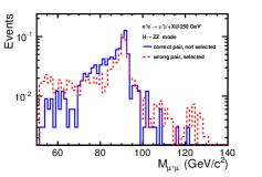
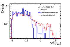
For each event, two isolated leptons of the same flavor and opposite charges are selected as the candidate pair for analysis. In this stage, it is essential to distinguish a pair of leptons produced in the decay of the Z boson recoiling against the Higgs boson (“correct pair”) from those produced in the Higgs boson decay (“wrong pair”). This is important for achieving precise $M_{\mathrm{H}}$ measurements and for preventing Higgs decay mode dependence. For the Higgsstrahlung process, the invariant mass $M_{\mathrm{l^{+}l^{-}}}$ ($\mathrm{l}$ = $\mathrm{e}$ or $\mathrm{\mu}$) of the dilepton system and recoil mass $M_{\mathrm{rec}}$ should be close to the Z boson mass $M_{\mathrm{Z}}$=91.187 GeV [18] and the Higgs boson mass $M_{\mathrm{H}}$=125 GeV (in this study), respectively. The decay modes which contain an extra source of leptons, such as the $\mathrm{H\rightarrow ZZ^{*}}$ and $\mathrm{H\rightarrow WW^{*}}$ modes, have a higher ratio of “wrong pairs”.

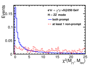
The best lepton pair candidate is selected based on the following criteria. First, the requirement $\left|M_{\mathrm{l^{+}l^{-}}}-M_{\mathrm{Z}}\right|<40(60)\>\mathrm{GeV}$ is implemented for $\mu\left(\mathrm{e}\right)$. In the case where both leptons originate from a single Z boson produced in Higgs boson decay, $M_{\mathrm{rec}}$ tends to deviate from $M_{\mathrm{H}}$ even if $M_{\mathrm{l^{+}l^{-}}}$ is close to $M_{\mathrm{Z}}$. Therefore the next step is to select, taking into account both $M_{\mathrm{l^{+}l^{-}}}$ and $M_{\mathrm{rec}}$, the pair which minimizes the following $\chi^{2}$ function:

$$\chi^{2}\left(M_{\mathrm{l^{+}l^{-}}},M_{\mathrm{rec}}\right)=\frac{\left(M_{\mathrm{l^{+}l^{-}}}-M_{\mathrm{Z}}\right)^{2}}{\sigma_{M_{\mathrm{l^{+}l^{-}}}}^{2}}+\frac{\left(M_{\mathrm{rec}}-M_{\mathrm{H}}\right)^{2}}{\sigma_{M_{\mathrm{rec}}}^{2}}\>,$$ (3)

$\sigma_{M_{\mathrm{l^{+}l^{-}}}}$ and $\sigma_{M_{\mathrm{rec}}}$ are determined by a Gaussian fit to the distributions of $M_{\mathrm{l^{+}l^{-}}}$ and $M_{\mathrm{rec}}$ for each channel. Using the $\mathrm{H\rightarrow ZZ^{*}}$ mode in the $\mathrm{\mu{}^{+}\mathit{\mu}^{-}H}$ channel at $\sqrt{s}$=250 GeV as an example, Figure 4 compares the distributions of $M_{\mathrm{l^{+}l^{-}}}$ and $M_{\mathrm{rec}}$ between “correct” (solide line) and “wrong” (dotted line) pairs, defined as those in which at least one lepton is from Higgs boson decay. Here, the “correct” and “wrong” pairs are separated using the MC truth information of the pairs selected by the above-mentioned pairing algorithm. One can see, only in the case of the “correct pairs”, a clean $M_{\mathrm{l^{+}l^{-}}}$ peak at $M_{\mathrm{Z}}$ signaling Z boson production, and a clean $M_{\mathrm{rec}}$ peak corresponding to the Higgs boson production. At $\sqrt{s}$ = 250 GeV, the efficiency of the dilepton finder described above in finding a pair of isolated leptons is about 94% and about 89% for the $\mathrm{\mu{}^{+}\mathit{\mu}^{-}H}$ and $\mathrm{e^{+}e^{-}H}$ channels, respectively. Meanwhile “wrong pairs” as well as the backgrounds in Section 3.3 are significantly suppressed.

The shape of the $M_{\mathrm{rec}}$ distribution is affected by radiative and resolution effects. The radiative effects comprise of beamstrahlung, Initial State Radiation (ISR), Final State Radiation (FSR) and bremsstrahlung. Because events are moved from the peak region of the $M_{\mathrm{rec}}$ distribution to the tail, the measurement precision is degraded. On the other hand, resolution effects determine the peak width of the distribution and thus the measurement uncertainties. The dominant resolution effects are the beam energy spread induced by the accelerator and the uncertainty of the detector response, dominated by the track momentum resolution. Compared to these, the SM Higgs decay width of about 4 MeV is negligible. While ISR and FSR are unsuppressible physical effects, beamstrahlung, bremsstrahlung, and resolution effects can be mitigated by optimization in the design of accelerator and detector.

Figure 4: Comparison of the distributions of $M_{\mathrm{l^{+}l^{-}}}$ (left) and $M_{\mathrm{rec}}$ (right) between “correct” and “wrong” lepton pairs. This is an example of the $\mathrm{H\rightarrow ZZ^{*}}$ decay mode in the $\mathrm{\mu{}^{+}\mathit{\mu}^{-}H}$ channel at $\sqrt{s}$ = 250 GeV.

4.2 Recovery of Bremsstrahlung and FSR Photons

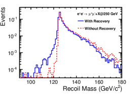
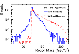
The bremsstrahlung and FSR of the final state leptons degrade measurement precision of $\sigma_{\mathrm{ZH}}$ and $M_{\mathrm{H}}$, particularly for the $\mathrm{e^{+}e^{-}H}$ channel, which has a broader peak and longer tail to lower values than the $\mathrm{\mu{}^{+}\mathit{\mu}^{-}H}$ channel. The recovery of bremsstrahlung and FSR photons is implemented for both $\mathrm{\mu{}^{+}\mathit{\mu}^{-}H}$ and $\mathrm{e^{+}e^{-}H}$ channels. A bremsstrahlung/FSR photon is identified using its polar angle with respect to the final state lepton; if the cosine of the polar angle exceeds 0.99, the photon four momentum is combined with that of the lepton. Figure 5 compares the reconstructed $M_{\mathrm{l^{+}l^{-}}}$ and $M_{\mathrm{rec}}$ spectra before (dotted line) and after (solid line) bremsstrahlung/FSR recovery for $\sqrt{s}$=250 GeV. It can be seen that the recovery process pushes the events at the lower end of the $M_{\mathrm{l^{+}l^{-}}}$ spectrum (corresponding to the tail in the higher region of the $M_{\mathrm{rec}}$ spectrum) back to the peak. In the case of the $\mathrm{e^{+}e^{-}H}$ channel, the precision of $\sigma_{\mathrm{ZH}}$ could become degraded by more than 50%, and $M_{\mathrm{H}}$ by more than 20% without the recovery process. The change in the $\mathrm{\mu{}^{+}\mathit{\mu}^{-}H}$ channel is negligible.

Figure 5: Comparison of the $M_{\mathrm{l^{+}l^{-}}}$ (top) and $M_{\mathrm{rec}}$ (bottom) spectra between the cases with (blue) and without (red) bremsstrahlung/FSR recovery for $\sqrt{s}$ = 250 GeV. The left and right shows the $\mathrm{\mu{}^{+}\mathit{\mu}^{-}H}$ and $\mathrm{e^{+}e^{-}H}$ channels, respectively.

4.3 Background rejection

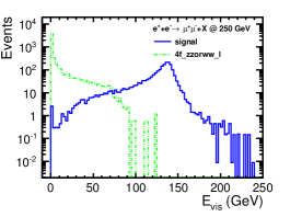
After the signal selection process, background events are rejected by applying cuts on various kinematic properties. While the cut values are adjusted for each center-of-mass energy, the overall strategies are similar. Unless specified otherwise, the plots in this section are made using the standard samples of the $\mathrm{\mu{}^{+}\mathit{\mu}^{-}H}$ channel and $\mathrm{\mathrm{e_{L}^{-}}\mathit{\mathrm{e_{R}^{+}}}}$ at $\sqrt{s}$=250 GeV, and are normalized to the assumed integrated luminosities, cross sections, and polarizations (see Section 3.3). In these plots, 4f_zz_l(sl) represents background with ZZ intermediate states and two pairs of $\mu\mu$ / $\tau\tau$ (a pair of $\mu\mu$ / $\tau\tau$ and a pair of quarks), 2f_z_l and 2f_bhabhag represents background with final states of $\mu\mu$ / $\tau\tau$ and $\mathrm{ee}$, respectively, and 4f_zzorww_l represents background with $\mu\mu\nu\nu$ or $\tau\tau\nu\nu$ as the final state. First, a loose precut on $M_{\mathrm{rec}}$ is applied as $M_{\mathrm{rec}}\in$[100, 300] GeV. Then the following cuts are applied in this order:

• since the invariant mass $M_{\mathrm{l^{+}l^{-}}}$ ($\mathrm{l}$ = $\mathrm{e}$ or $\mu$) of the dilepton system should be close to the Z boson mass for the Higgsstrahlung process, a criterion is imposed as $M_{\mathrm{l^{+}l^{-}}}\in$[73, 120] GeV. The top left plot in Figure 6 compares the $M_{\mathrm{l^{+}l^{-}}}$ of signal and major background processes.

• for the signal, the transverse dilepton momentum $p_{\mathrm{T}}^{\mathrm{l^{+}l^{-}}}$ should peak at a certain value determined by kinematics. In contrast, the $p_{\mathrm{T}}^{\mathrm{l^{+}l^{-}}}$ of 2-fermion background peaks towards small values. This motivates the cut $p_{\mathrm{T}}^{\mathrm{l^{+}l^{-}}}$> 10 GeV. In addition, an upper limit on $p_{\mathrm{T}}^{\mathrm{l^{+}l^{-}}}$ is imposed to suppress background processes whose $p_{\mathrm{T}}^{\mathrm{l^{+}l^{-}}}$ extend to large values. The top right plot in Figure 6 compares the $p_{\mathrm{T}}^{\mathrm{l^{+}l^{-}}}$ of the signal and major background processes.

• $\theta_{\mathrm{missing}}$, the polar angle of the missing momentum, discriminates against events which are unbalanced in longitudinal momentum, in particular those 2-fermion events in which ISR emitted approximately collinear with the incoming beams escapes detection in the beam pipe. The bottom left plot in Figure 6 shows the distribution of $\mathrm{cos\left(\theta_{missing}\right)}$ between the signal and major background processes. A cut is made at $\mathrm{\left|cos\left(\theta_{missing}\right)\right|}<0.98$, which cuts 2f_l background by approximately two thirds.

• multi-variate cut: While the $p_{\mathrm{T}}^{\mathrm{l^{+}l^{-}}}$ and $\mathrm{cos\left(\theta_{missing}\right)}$ cuts are effective for removing 2-fermion background, the signatures of 4-fermion backgrounds are harder to distinguish from the Higgsstrahlung signal, especially in the case of one of the dominant background processes $\mathrm{\mathrm{\mathrm{\mathrm{e^{+}\mathrm{e^{-}}}\rightarrow ZZ\rightarrow\mathit{\mathrm{llqq}}}}}$ ($l$=$\mathrm{e}$ or $\mu$). Nevertheless, further rejection of residual background events is achieved by a multi-variate (MVA) cut based on the Boosted Decision Tree (BDT) method [20] using a combination of the variables $M_{\mathrm{l^{+}l^{-}}}$, $\mathrm{cos\left(\theta_{Z}\right)}$, $\mathrm{cos\left(\theta_{lep}\right)}$, $\mathrm{cos\left(\theta_{track,1}\right)}$ and $\mathrm{cos\left(\theta_{track,2}\right)}$. Here, $\theta_{\mathrm{Z}}$ is the polar angle of the Z boson, $\theta_{\mathrm{lep}}$ is the angle between the leptons, and $\theta_{\mathrm{track,1,2}}$ is the polar angle of each lepton track. The BDT response is calculated using weights obtained from training samples consisting of simulated signal and background events. The MVA cut is optimized for each channel to maximize $\sigma_{\mathrm{ZH}}$ precision, and is very effective for increasing signal significance. For example, in the case of the $\mathrm{\mu{}^{+}\mathit{\mu}^{-}H}$ channel at $\sqrt{s}$=250 GeV, the number of background events is reduced by more than 35% by the MVA cut, whereas the loss of signal events is only about 5%.

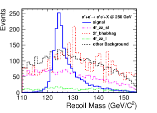
• recoil mass cut: $\sigma_{\mathrm{ZH}}$ and $M_{\mathrm{H}}$ are obtained by fitting the $M_{\mathrm{rec}}$ spectrum within a wide window around the signal $M_{\mathrm{rec}}$ peak. This is designated to be $M_{\mathrm{rec}}\in$[110, 155] GeV for $\sqrt{s}$=250 GeV, [100, 200] GeV for $\sqrt{s}$=350 GeV, and [100, 250] GeV for $\sqrt{s}$= 500 GeV.

• visible energy cut: $E_{\mathrm{vis}}$, defined as the visible energy excluding that from the isolated lepton pair, is required to be above a certain value (10 GeV for $\sqrt{s}$=250 and 350 GeV and 25 GeV for $\sqrt{s}$=500 GeV) in order to suppress one of the dominant residual backgrounds which has $\mathrm{ll\nu\nu}$ ($\mathrm{l}$ = $\mathrm{e}$ or $\mu$) in the final state. The bottom right plot in Figure 6 compares the distributions of $E_{\mathrm{vis}}$ between signal and $\mathrm{ll\nu\nu}$ background. For example, in the case of the $\mathrm{\mu{}^{+}\mathit{\mu}^{-}H}$ channel at $\sqrt{s}$=250 GeV, the $\mathrm{ll\nu\nu}$ background occupies about 30% and 10% of all residual backgrounds without and with the $E_{\mathrm{vis}}$ cut, respectively. This reduces background events by 30-50% and further improves the precision on $\sigma_{\mathrm{ZH}}$ and $M_{\mathrm{H}}$ by 10-15% in the case of the $\mathrm{\mathrm{e_{L}^{-}}\mathit{\mathrm{e_{R}^{+}}}}$ polarization[Modedependence], where the contribution of $\mathrm{ll\nu\nu}$ background with WW intermediate states is significant. Although the $E_{\mathrm{vis}}$ cut also excludes signal events in which the Higgs boson decays invisibly, Higgs decay model independence is maintained by combining the results obtained from this analysis with a dedicated analysis for invisible Higgs decays [21, 22]. This is explained by the fact that the $\mathrm{ZH}$ cross section for the SM Higgs boson can be expressed as $\sigma_{\mathrm{ZH}}=\sigma_{\mathrm{ZH,vis}}+\sigma_{\mathrm{\mathrm{ZH,inv}is}}$, where $\sigma_{\mathrm{ZH,vis}}$ and $\sigma_{\mathrm{ZH,invis}}$ , which are the cross sections of the visible and invisible decay events, respectively, can both be measured individually and model independently.

For the case of the $\mathrm{\mu{}^{+}\mathit{\mu}^{-}H}$ channel at $\sqrt{s}$= 250 GeV, Table 3 shows the number of remaining signal and background, signal efficiency and significance after each cut. Similar outcomes are seen for $\sqrt{s}$=350 and 500 GeV since similar data selection methods are used. Figure 7 shows distributions of the $M_{\mathrm{rec}}$ of signal and major residual background processes for $\sqrt{s}$=250 GeV. The major residual backgrounds are 4f_sl and 2f_l defined in Section 3.3.

Figure 6: (top left) The $M_{\mu^{+}\mu^{-}}$ distributions of signal and the major background processes, after a loose precut on $M_{\mathrm{rec}}$. (top right) The $p_{\mathrm{\mathrm{T}}}^{\mu^{+}\mu^{-}}$ distributions of signal and the major background processes, after a loose precut on $M_{\mathrm{rec}}$ and a cut on $M_{\mu^{+}\mu^{-}}$. (bottom left) The $\mathrm{cos\left(\theta_{missing}\right)}$ distributions of signal and 2-fermion background, after a loose precut on $M_{\mathrm{rec}}$ and cuts have been applied on $M_{\mu^{+}\mu^{-}}$ and $p_{\mathrm{\mathrm{T}}}^{\mu^{+}\mu^{-}}$. (bottom right) The distributions of $E_{\mathrm{vis}}$ (after excluding the dilepton energy) of the signal and the 4f_zzorww_l processes, after a loose precut on $M_{\mathrm{rec}}$ and cuts have been applied on $M_{\mu^{+}\mu^{-}}$, $p_{\mathrm{\mathrm{T}}}^{\mu^{+}\mu^{-}}$., $\mathrm{cos\left(\theta_{missing}\right)}$, and the BDT response of the MVA analysis.

$\int\mathcal{L}dt$	$\mathrm{\mu{}^{+}\mathit{\mu}^{-}H}$	signal	signal				total
250 $\mathrm{fb^{-1}}$	$\mathrm{e_{L}^{-}e_{R}^{+}}$	efficiency	significance	2f_l	4f_l	4f_sl	background
no cut	2603	100%	0.42	9.54$\times 10^{6}$	3.15$\times 10^{6}$	4.98$\times 10^{6}$	1.98$\times 10^{7}$
Lepton ID+Precut	2439	93.70%	7.46	61675	34451	8218	104344
$M_{\mathrm{l^{+}l^{-}}}\in$[73, 120] GeV	2382	91.51%	8.09	54352	22543	7446	84341
$p_{\mathrm{T}}^{\mathrm{l^{+}l^{-}}}\in$[10, 70] GeV	2335	89.70%	11.17	15429	19648	6245	41322
$\mathrm{\left|cos\mathit{\theta_{\mathrm{missing}}}\right|}$< 0.98	2335	89.70%	12.71	5594	19539	6245	31378
MVA	2310	88.74%	15.03	4195	12530	4586	21311
$M_{\mathrm{rec}}\in$[110, 155] GeV	2296	88.21%	16.37	3522	10423	3433	17378
$E_{\mathrm{vis}}$ > 10 GeV	2293	88.09%	20.94	3261	2999	3433	9694

Table 3: The number of events left after each cut for the $\mathrm{\mu{}^{+}\mathit{\mu}^{-}H}$ channel and $\mathrm{e_{L}^{-}e_{R}^{+}}$ at $\sqrt{s}$=250 GeV. Also given are the efficiency and signal significance (defined as $\frac{N_{S}}{\sqrt{N_{S}+N_{B}}}$ ,where $N_{S(B)}$ is the number of signal (background)) for the Higgsstrahlung signal. Precut represents the loose cut $M_{\mathrm{rec}}\in$[100, 300] GeV.

Figure 7: The histograms of the recoil mass of the signal and the major residual background processes left in a wide window around the signal $M_{\mathrm{rec}}$ peak, shown here for the $\mathrm{\mu{}^{+}\mathit{\mu}^{-}H}$ (left) and $\mathrm{e{}^{+}\mathrm{\mathrm{\mathit{\mathrm{e}}^{-}}}H}$ (right) channels at $\sqrt{s}$=250 GeV, after all cuts described in the main text have been applied.

5 DEMONSTRATION OF HIGGS DECAY MODE INDEPENDENCE

In the recoil method, $\sigma_{\mathrm{ZH}}$ is measured without any explicit assumption regarding Higgs decay modes. This section demonstrates that the $\sigma_{\mathrm{ZH}}$ measured using the methods described in [6] based on the data selection in Section 4 does not depend on the underlying model which determines the Higgs decay modes and their branching ratios. As can be understood from Equation 2, the key question here is whether the $\sigma_{\mathrm{ZH}}$ extracted using the measured number of signal events ($N_{\mathrm{S}}$) and the signal selection efficiency ($\varepsilon_{\mathrm{S}}$) from the Monte Carlo samples would be biased when the Higgs boson decays differently from that assumed in the samples.

5.1 General strategies towards model independence

First we introduce the general strategies towards a model independent $\sigma_{\mathrm{ZH}}$ measurement. The direct observable $N_{\mathrm{S}}$ can be parameterised as

$$N_{\mathrm{S}}=\underset{i}{\varSigma}N_{i}=\underset{i}{\varSigma}\sigma_{\mathrm{ZH}}R_{l}LB_{i}\varepsilon_{i}\,,$$ (4)

where the summation goes through all Higgs decay modes. $N_{\mathrm{i}}$, $B_{\mathrm{i}}$, and $\varepsilon_{\mathrm{i}}$ are the the number of signal events, branching ratio and selection efficiency of Higgs decay mode $i$, respectively. $L$ is the integrated luminosity, and $R_{l}$ is the branching ratio of $\mathrm{Z\rightarrow l^{+}l^{-}}$. If the signal efficiency equals to the same $\varepsilon$ for all decay modes, Equation 4 becomes

$$N_{\mathrm{S}}=\sigma_{\mathrm{ZH}}R_{l}L\varepsilon\underset{i}{\varSigma}B_{i}\,.$$ (5)

Since $\underset{i}{\varSigma}B_{i}=1$ stands in any case, $\sigma_{\mathrm{ZH}}$ can be extracted without assumptions on decay modes or branching ratios as

$$\sigma_{\mathrm{ZH}}=\frac{N_{\mathrm{S}}}{R_{l}L\varepsilon}\,,$$ (6)

This is the ideal case which guarantees model independence. On the other hand, if there exist discrepancies between the signal efficiencies of each mode, $\sigma_{\mathrm{ZH}}$ has to be extracted as

$$\sigma_{\mathrm{ZH}}=\frac{N_{\mathrm{S}}}{R_{l}L\underset{i}{\varSigma}B_{i}\varepsilon_{i}}\equiv\frac{N_{\mathrm{S}}}{R_{l}L\overline{\varepsilon}}\,,$$ (7)

where $\overline{\varepsilon}=\underset{i}{\varSigma}B_{i}\varepsilon_{i}$ is the expected efficiency for all decay modes. In this case, the bias on $\sigma_{\mathrm{ZH}}$ depends on the determination of $\overline{\varepsilon}$. This is discussed as follows in terms of three possible scenarios of our knowledge of Higgs decay at the time of $\sigma_{\mathrm{ZH}}$ measurement.

• scenario A: all Higgs decay modes and the corresponding $B_{i}$ for each mode are known. In this rather unlikely case, $\overline{\varepsilon}$ can be determined simply by summing up over all modes, leaving no question of model independence.

• scenario B: $B_{i}$ is completely unknown for every mode. We would examine the discrepancy in $\epsilon_{i}$ by investigating as many modes as possible, and retrieve the maximum and minimum of $\epsilon_{i}$ as $\varepsilon_{\mathrm{min}}\leq\epsilon_{i}\leq\varepsilon_{\mathrm{max}}$, from which $\overline{\varepsilon}$ can be constrained as $\varepsilon_{\mathrm{min}}\underset{i}{\Sigma}B_{i}\leq\overline{\varepsilon}\leq\varepsilon_{\mathrm{max}}\underset{i}{\Sigma}B_{i}$. Given that $\underset{i}{\varSigma}B_{i}=1$, this can be rewritten as $\varepsilon_{\mathrm{min}}\leq\overline{\varepsilon}\leq\varepsilon_{\mathrm{max}}$. Then from Equation 7, $\sigma_{\mathrm{ZH}}$ can be constrained as

$$\frac{N_{\mathrm{S}}}{R_{l}L\varepsilon_{\mathrm{max}}}\leq\sigma_{\mathrm{ZH}}\leq\frac{N_{\mathrm{S}}}{R_{l}L\varepsilon_{\mathrm{min}}}\,,$$ (8)

which indicates that the possible relative bias on $\sigma_{\mathrm{ZH}}$ can be estimated as $\frac{\varepsilon_{\mathrm{\mathrm{max}}}-\varepsilon_{\mathrm{min}}}{\varepsilon_{\mathrm{\mathrm{max}}}+\varepsilon_{\mathrm{min}}}$. This scenario is based on a considerably conservative assumption.

• scenario C: $B_{i}$ is known for some of the decay modes. Here, it is assumed that the decay modes $i$ = 1 to $n$ with a total branching ratio of $B_{0}=\stackrel{{\scriptstyle[}}{{i}}=1]{n}{\Sigma}B_{i}$ are known, and that the modes from $i$ = $n+1$ with a total branching ratio of $B_{x}=\underset{i=n+1}{\Sigma}B_{i}$ are unknown. In this case, we would know the efficiency of the known modes as $\varepsilon_{0}=\frac{\stackrel{{\scriptstyle[}}{{i}}=1]{n}{\Sigma}B_{i}\varepsilon_{i}}{B_{0}}$. Meanwhile the efficiency for each unknown mode can be expressed as $\varepsilon_{i}=\varepsilon_{0}+\delta\varepsilon_{i}$, where $\delta\varepsilon_{i}$ is the deviation in efficiency for each unknown mode $i$ from $\varepsilon_{0}$. We can then write $\overline{\varepsilon}$ as

$$\overline{\varepsilon}=\stackrel{{\scriptstyle[}}{{i}}=1]{n}{\Sigma}B_{i}\varepsilon_{i}+\underset{i=n+1}{\Sigma}B_{i}\varepsilon_{i}=B_{0}\varepsilon_{0}+B_{x}\varepsilon_{0}+\underset{i=n+1}{\Sigma}B_{i}\delta\varepsilon_{i}=\varepsilon_{0}+\underset{i=n+1}{\Sigma}B_{i}\delta\varepsilon_{i}\,.$$ (9)

The relative bias for $\overline{\varepsilon}$ and hence for $\sigma_{\mathrm{ZH}}$ is a combination of the contribution from the unknown modes and the known modes. The contribution from the unknown modes is derived as

$$\frac{\Delta\sigma_{\mathrm{ZH}}}{\sigma_{\mathrm{ZH}}}=\frac{\Delta\overline{\varepsilon}}{\overline{\epsilon}}<\underset{i=n+1}{\Sigma}B_{i}\frac{\delta\varepsilon_{\mathrm{max}}}{\varepsilon_{0}}=B_{x}\frac{\delta\varepsilon_{\mathrm{max}}}{\varepsilon_{0}}\,,$$ (10)

where $\delta\varepsilon_{\mathrm{max}}$ is the maximum of $\left|\delta\varepsilon_{i}\right|$ for the unknown modes. As for the known modes, because $\overline{\varepsilon}=\stackrel{{\scriptstyle[}}{{i}}=1]{n}{\Sigma}B_{i}\varepsilon_{i}=\stackrel{{\scriptstyle[}}{{i}}=1]{n}{\Sigma}B_{i}\left(\varepsilon_{0}+\delta\varepsilon_{i}\right)$, where $\delta\varepsilon_{i}\equiv\varepsilon_{i}-\varepsilon_{0}$ is the deviation in efficiency for each known mode, the uncertainty due to a fluctuation in their branching ratios ($\Delta B_{i}$) can be expressed as $\Delta\overline{\varepsilon}=\stackrel{{\scriptstyle[}}{{i}}=1]{n}{\Sigma}\Delta B_{i}\varepsilon_{0}+\stackrel{{\scriptstyle[}}{{i}}=1]{n}{\Sigma}\Delta B_{i}\delta\varepsilon_{i}=\stackrel{{\scriptstyle[}}{{i}}=1]{n}{\Sigma}\Delta B_{i}\delta\varepsilon_{i}$. Therefore the contribution from the known modes is derived as

$$\frac{\Delta\sigma_{\mathrm{ZH}}}{\sigma_{\mathrm{ZH}}}=\frac{\Delta\overline{\varepsilon}}{\overline{\epsilon}}=\sqrt{\stackrel{{\scriptstyle[}}{{i}}=1]{n}{\Sigma}\Delta B_{i}^{2}\left(\frac{\varepsilon_{i}}{\varepsilon_{0}}-1\right)^{2}}\,.$$ (11)

Scenario C is the most realistic as we will certainly have branching ratio measurements from both the LHC and the ILC itself for a wide range of Higgs decay modes.

From the above formulation, it is apparent that the key to maintaining model independence is to minimize the discrepancies in signal efficiency between decay modes. The data selection methods in Section 4 are designed to satisfy this purpose while still achieving high precision of $\sigma_{\mathrm{ZH}}$ and $M_{\mathrm{H}}$. To cover a large number of Higgs decay modes and monitor their efficiencies, high statistics signal samples ($\sim$ 40k events) are produced for each major SM decay modes ($\mathrm{H\rightarrow\mathrm{bb}}$, cc, gg, $\tau\tau$, $\mathrm{WW^{*}}$, $\mathrm{ZZ^{*}}$, $\gamma\gamma$, $\gamma\mathrm{Z}$), and for each beam polarisation and center-of-mass energy, so that the relative statistical error of each efficiency is below 0.2% in the end for any channel.

5.2 Analysis strategies

5.2.1 Algorithms for lepton pairing

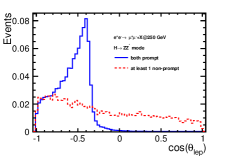
The efforts to minimize bias start from the very beginning of the data selection process. The isolated lepton selection mentioned in Section 4.1.1 is tuned to take into account the fact that each decay mode has a different density of particles surrounding the leptons from Z boson decay. Section 4.1.2 mentioned that the decay modes which contain an extra source of leptons receive the effect from “lepton pairing mistake”, defined as the case in which at least one of the leptons in the selected dilepton pair is from Higgs boson decay. The analysis in [6] pairs leptons using a method which minimizes a function $\chi^{2}\left(M_{\mathrm{l^{+}l^{-}}},M_{\mathrm{r\mathrm{ec}}}\right)$ (Equation 3). Figure 8 shows the distribution of $\chi^{2}\left(M_{\mathrm{l^{+}l^{-}}},M_{\mathrm{r\mathrm{ec}}}\right)$ at $\sqrt{s}$=250 GeV. In this section, this “$\chi^{2}$ method” will be compared to two other types of lepton pairing algorithm. One is the “$M_{\mathrm{l^{+}l^{-}}}$ method”, which selects the pair of leptons with $M_{\mathrm{l^{+}l^{-}}}$ closest to $M_{\mathrm{Z}}$ as the signal dilepton. The shortcoming of the $M_{\mathrm{l^{+}l^{-}}}$ method is that when both leptons are from the same Z boson originating from Higgs decay, their $M_{\mathrm{l^{+}l^{-}}}$ would still be close to $M_{\mathrm{Z}}$, whereas the corresponding $M_{\mathrm{rec}}$ tend to be deviated from $M_{\mathrm{H}}$. Another one is the “MVA method”, which selects a pair of leptons that maximizes a MVA response formed from $M_{\mathrm{Z}}$ , $M_{\mathrm{rec}}$, $\cos\theta_{\mathrm{Z}}$, $\cos\theta_{\mathrm{lep}}$, and $p_{\mathrm{\mathrm{Z}}}$. The MVA evaluation is done using the MLP method and the weights are trained using the $\mathrm{H\rightarrow ZZ^{*}}$ mode sample which has the highest probability of wrong pairing. Figure 9 compares the distribution of the MVA variables between correct and wrong pairs. Regarding $M_{\mathrm{Z}}$ and $M_{\mathrm{rec}}$, $\cos\theta_{\mathrm{lep}}$, and $p_{\mathrm{\mathrm{Z}}}$, those of the correct pairs peak around the value calculated from kinematics whereas those of the wrong pairs have a wider distribution. Regarding $\cos\theta_{\mathrm{Z}}$, correct pairs have a more isotropic distribution than wrong pairs.

Figure 8: The distribution of $\chi^{2}\left(M_{\mathrm{l^{+}l^{-}}},M_{\mathrm{r\mathrm{ec}}}\right)$ of the “correct” and “wrong” lepton pairs in the $\mathrm{H\rightarrow ZZ^{*}}$ mode, shown for the $\mathrm{\mu{}^{+}\mathit{\mu}^{-}H}$ channel and $\mathrm{e_{L}^{-}e_{R}^{+}}$ at $\sqrt{s}$ = 250 GeV.

Figure 9: The distribution of the variables $M_{\mathrm{l^{+}l^{-}}}$, $M_{\mathrm{rec}}$, $p_{\mathrm{\mathrm{Z}}}$ , $\cos\theta_{\mathrm{Z}}$, and $\cos\theta_{\mathrm{lep}}$ used for the training in the MVA lepton pairing method, shown here for the “correct pairs” and “wrong pairs” in the case of the $\mathrm{\mu{}^{+}\mathit{\mu}^{-}H}$ channel and and $\mathrm{e_{L}^{-}e_{R}^{+}}$ at $\sqrt{s}$ = 250 GeV.

Prior to pairing the leptons, a pre-cut on $M_{\mathrm{l^{+}l^{-}}}$ is implemented as $\left|M_{\mathrm{l^{+}l^{-}}}-M_{\mathrm{Z}}\right|<40(60)\>\mathrm{GeV}$ for $\mu\left(\mathrm{e}\right)$. For each of the three methods, Table 5 shows the pairing performance for the $\mathrm{H\rightarrow ZZ^{*}}$ mode. The ratios are defined with respect to the number of generated events. The MC statistical uncertainty is about 0.1%. It can be observed that there is no significant difference between the $\chi^{2}$ method, which was eventually used in analysis, and the MVA method, while both are better than the $M_{\mathrm{l^{+}l^{-}}}$ method. The pairing performance at $\sqrt{s}$=250 GeV using the $\chi^{2}$ method is shown for all major SM Higgs decay modes in Appendix B.

C0	number of generated events
C1	number of selected $\mu$ (e) for $\mathrm{\mu{}^{+}\mathit{\mu}^{-}H}$ ($\mathrm{\mathrm{e}{}^{+}\mathit{\mathrm{e}}^{-}H}$) channel
C2	correct pairs
C3	1 prompt and 1 non-prompt lepton selected, with 2 prompt leptons found
C4	2 non-prompt leptons selected, with 2 prompt leptons found
C5	only 1 prompt lepton found
C6	no prompt leptons found

Table 4: The categorization of the lepton pairing performance for the recoil analysis.

$\sqrt{s}$=250 GeV		$\mathrm{\mu{}^{+}\mathit{\mu}^{-}H}$			$\mathrm{\mathrm{e}{}^{+}\mathit{\mathrm{e}}^{-}H}$
$\mathrm{H\rightarrow ZZ^{*}}$	$\chi^{2}$	MVA	$M_{\mathrm{l^{+}l^{-}}}$	$\chi^{2}$	MVA	$M_{\mathrm{l^{+}l^{-}}}$
C0	100%	100%	100%	100%	100%	100%
C1	94.15%	94.15%	94.15%	87.08%	87.08%	87.08%
C2	93.17%	93.18%	92.44%	85.13%	85.09%	84.78%
C3	0.728%	0.715%	1.46%	1.363%	1.412%	1.714%
C4	0.342%	0.421%	1.13%	0.548%	0.795%	1.017%
C5	0.250%	0.250%	0.250%	0.572%	0.572%	0.572%
C6	0.002%	0.002%	0.002%	0.008%	0.008%	0.008%

Table 5: The lepton pairing performance of the $\mathrm{H\rightarrow ZZ^{*}}$ mode and and $\mathrm{e_{L}^{-}e_{R}^{+}}$ at $\sqrt{s}$=250 GeV. The categories C1-C6 are defined in Table 4. The statistical uncertainties are below 0.1%.

From Figure8, it can be seen that while correct pair events peak sharply at a small $\chi^{2}\left(M_{\mathrm{l^{+}l^{-}}},M_{\mathrm{rec}}\right)$ value, about 1/10 of the peak is occupied by wrong pair events, which explains the finite amount of pairing mistakes. The fact that this can not be visibly improved by the MVA method can be understood from Figure10 which compares the variables $M_{\mathrm{l^{+}l^{-}}}$, $M_{\mathrm{rec}}$ ,$p_{\mathrm{\mathrm{Z}}}$ , $\cos\theta_{\mathrm{Z}}$, and $\cos\theta_{\mathrm{lep}}$ of the following two types of events: (A) A pair consisting of two leptons from the Z boson recoiling against the Higgs boson, whereas the actually “selected pair ” contains at least one lepton from Higgs decay, and (B) A “selected pair” consisting of at least one lepton from Higgs decay. With the exception that the distributions of $p_{\mathrm{\mathrm{Z}}}$ and $M_{\mathrm{rec}}$ are slightly wider for (B), there is no significance difference between (A) and (B).

Figure 10: The distribution of $M_{\mathrm{l^{+}l^{-}}}$, $M_{\mathrm{rec}}$, $p_{\mathrm{\mathrm{Z}}}$, $\cos\theta_{\mathrm{Z}}$ and $\cos\theta_{\mathrm{lep}}$ of the “correct pairs” which did not get selected, and the “wrong pairs” which got selected, shown for the $\mathrm{H\rightarrow ZZ^{*}}$ mode, $\mathrm{\mathrm{\mu}{}^{+}\mathit{\mathrm{\mu}}^{-}H}$ channel and $\mathrm{e_{L}^{-}e_{R}^{+}}$ at $\sqrt{s}$=250 GeV.

5.2.2 Other sources of bias

Following the selection of the isolated lepton pairs, the cuts on $M_{\mathrm{l^{+}l^{-}}}$, $p_{\mathrm{T}}^{\mathrm{l^{+}l^{-}}}$, BDT, and $M_{\mathrm{rec}}$ are designed to use only kinematical information from the selected leptons so as to avoid introducing bias to the efficiencies of individual Higgs decay modes. On the other hand, the $\cos\left(\theta_{\mathrm{missing}}\right)$ cut, which counts the missing momentum from the whole event, in principle uses information of particles from Higgs decay. The $E_{\mathrm{vis}}$ cut will not introduce additional bias, as it simply categorizes the events into visible or invisible Higgs decay, as mentioned in Section 4.3.

Tables 6 and 7 show the efficiency of each decay mode after each cut for the case of $\sqrt{s}$=250 GeV and $\mathrm{e_{L}^{-}e_{R}^{+}}$. The tables for the other channels are given in Appendix C. The bias is reduced at higher center-of-mass energies. For example, at $\sqrt{s}$=500 GeV, no bias exists beyond the MC statistical error (< 0.2%) for any mode. Based on these results, the bias on the measured $\sigma_{\mathrm{ZH}}$ will be given in Section5.3. The following sources of residual bias can be observed:

• The first row “Lepton Finder” in the Tables 6 and 7 shows that more lepton pairs are found for the $\mathrm{H\rightarrow WW^{*}}$, $\mathrm{ZZ^{*}}$, $\mathrm{\tau\tau}$, and $\mathrm{\gamma Z}$ modes as they contain leptons from Higgs decay as an extra source of leptons. These efficiencies are slightly evened out later on by “Lepton ID” and cuts on $M_{\mathrm{l^{+}l^{-}}}$ and $M_{\mathrm{rec}}$. On the other hand, the $\mathrm{H\rightarrow gg}$ mode has a slightly lower efficiency of finding isolated leptons due to the existence of widely spread gluon jets. This effect has already been minimized by using a $\mathrm{H\rightarrow gg}$ sample to train the MVA weights in the isolated lepton finder.

• The $\mathrm{H\rightarrow\gamma Z}$ mode receives bias from mistaken lepton ID due to the confusion with the leptons from Higgs decay. For example, in the $\mathrm{\mu^{+}\mu^{-}X}$ channel, a pair of electrons decayed from the Z boson from Higgs decay become selected as an isolated electron pair.

• The $\mathrm{H\rightarrow\gamma Z}$ mode receives bias from the $\cos\left(\theta_{\mathrm{missing}}\right)$ cut since it contains events with ISR photons going down the beam pipe but little visible energy other than that of the isolated lepton pair. The $\cos\left(\theta_{\mathrm{missing}}\right)$ cut is designed to be very loose so that this bias is very small, while 2-fermion backgrounds can still be suppressed effectively.

• The $\mathrm{H\rightarrow\gamma\gamma}$ mode in the $\mathrm{\mathrm{e}^{+}\mathrm{e}^{-}X}$ channel receives a slight bias from pre-cuts on $M_{\mathrm{rec}}$ due to the FSR/bremsstrahlung process (see Section LABEL:sub:FSR-Recovery). From Figure 11, a bump can be seen in the lower region of the reconstructed $M_{\mathrm{rec}}$ spectrum ($\lesssim$ 100 GeV) for the $\mathrm{H\rightarrow\gamma\gamma}$ mode; in these events the relatively energetic photons from Higgs decay are mistakenly recovered to the isolated leptons. This effect is less significant at higher center-of-mass energies for which the Higgs decay products are more boosted.

Figure 11: A comparison of $M_{\mathrm{rec}}$ between the decay modes $\mathrm{H\rightarrow\mathrm{bb}}$, gg, $\mathrm{WW^{*}}$, $\gamma\gamma$ and $\gamma\mathrm{Z}$ for the $\mathrm{\mathrm{e}{}^{+}\mathit{\mathrm{e}}^{-}H}$ channel and $\mathrm{e_{L}^{-}e_{R}^{+}}$ at $\sqrt{s}$ = 250 GeV.

$\mathrm{H\rightarrow XX}$	bb	cc	gg	$\tau\tau$	$\mathrm{\mathrm{WW^{*}}}$	$\mathrm{ZZ^{*}}$	$\gamma\gamma$	$\gamma\mathrm{Z}$
BR (SM)	57.8%	2.7%	8.6%	6.4%	21.6%	2.7%	0.23%	0.16%
Lepton Finder	93.70%	93.69%	93.40%	94.02%	94.04%	94.36%	93.75%	94.08%
Lepton ID+Precut	93.68%	93.66%	93.37%	93.93%	93.94%	93.71%	93.63%	93.22%
$M_{\mathrm{l^{+}l^{-}}}\in$[73, 120] GeV	89.94%	91.74%	91.40%	91.90%	91.82%	91.81%	91.73%	91.47%
$p_{\mathrm{t}}^{\mathrm{l^{+}l^{-}}}\in$[10, 70] GeV	89.94%	90.08%	89.68%	90.18%	90.04%	90.16%	89.99%	89.71%
$\mathrm{\left|cos\mathit{\theta_{\mathrm{missing}}}\right|}$< 0.98	89.94%	90.08%	89.68%	90.16%	90.04%	90.16%	89.91%	89.41%
MVA	88.90%	89.04%	88.63%	89.12%	88.96%	89.11%	88.91%	88.28%
$M_{\mathrm{rec}}\in$[110, 155] GeV	88.25%	88.35%	87.98%	88.43%	88.33%	88.52%	88.21%	87.64%

Table 6: The BR values and the efficiency of the major SM Higgs decay modes, after each data selection step, shown here for the case of the $\mathrm{\mu^{+}\mu^{-}X}$ channel and $\mathrm{e_{L}^{-}e_{R}^{+}}$ at $\sqrt{s}$=250 GeV. The statistical uncertainties on these values are below 0.16%.

$\mathrm{H\rightarrow XX}$	bb	cc	gg	$\tau\tau$	$\mathrm{\mathrm{WW^{*}}}$	$\mathrm{ZZ^{*}}$	$\gamma\gamma$	$\gamma\mathrm{Z}$
BR (SM)	57.8%	2.7%	8.6%	6.4%	21.6%	2.7%	0.23%	0.16%
Lepton Finder	89.12%	88.92%	88.51%	89.50%	89.87%	90.15%	89.83%	90.06%
Lepton ID+Precut	88.58%	88.42%	87.99%	88.58%	88.96%	88.37%	87.59%	87.67%
$M_{\mathrm{l^{+}l^{-}}}\in$[73, 120] GeV	86.70%	86.42%	85.94%	86.12%	86.19%	86.12%	85.38%	85.64%
$p_{\mathrm{t}}^{\mathrm{l^{+}l^{-}}}\in$[10, 70] GeV	84.96%	84.76%	84.24%	84.42%	84.47%	84.32%	83.65%	83.77%
$\mathrm{\left|cos\mathit{\theta_{\mathrm{missing}}}\right|}$< 0.98	84.96%	84.76%	84.24%	84.29%	84.45%	84.18%	83.24%	83.48%
MVA	68.90%	68.87%	68.52%	68.34%	68.19%	68.31%	67.39%	67.73%
$M_{\mathrm{rec}}\in$[110, 155] GeV	68.61%	68.60%	68.19%	68.04%	67.88%	68.02%	67.08%	67.45%

Table 7: The BR values and the efficiency of the major SM Higgs decay modes, after each data selection step, shown here for the case of the $\mathrm{\mathrm{e}^{+}\mathrm{e}^{-}X}$ channel and $\mathrm{e_{L}^{-}e_{R}^{+}}$ at $\sqrt{s}$=250 GeV. The statistical uncertainties on these values are below 0.16%.

5.3 Bias on the measured cross section

In this section, the potential bias on the measured $\sigma_{\mathrm{ZH}}$ due to residual Higgs decay mode dependence is evaluated from a conservative perspective. Table 6 shows no discrepancy in efficiencies beyond 1%, which demonstrates model independence at a level of better than 0.5% based on the most conservative scenario B. Note that the bias is even smaller at higher center-of-mass energies.

Regarding the most realistic scenario C, the bias is estimated as follows (using Equations 10 and 11). The known modes are assumed to be $\mathrm{H\rightarrow\mathrm{bb}}$, cc, gg, $\tau\tau$, $\mathrm{WW^{*}}$, $\mathrm{ZZ^{*}}$, $\gamma\gamma$, $\gamma\mathrm{Z}$, since they will be measured at the LHC or the ILC [26, 27]. Taking into consideration the possibility of unknown exotic Higgs decay modes, their total branching ratio ($B_{x}$) is assumed to be 10%, based on the estimation of the 95% C.L. upper limit for branching ratio of BSM decay modes from the HL-LHC [26]. In fact assigning a large BR of 10% to unknown modes is a considerably conservative assumption, because at the ILC the upper limit for BSM decay will be greatly improved and in general any decay mode with a few percent branching ratio shall be directly measured. Since the characteristics of any exotic decay mode is expected to fall within the wide range of known decay modes being directly investigated, we obtain $\delta\varepsilon_{\mathrm{max}}$ by assuming that the efficiencies of the unknown modes will lie in the range of the efficiencies of known modes; this is, for example, -0.68% from the $\gamma\mathrm{Z}$ mode in the case of the channel shown in Table 6. Then for the known modes, each $B_{i}$ is scaled from their SM values by 90%, following which $\varepsilon_{0}$ is obtained straightforwardly from $B_{i}$ and $\epsilon_{i}$. Each $\Delta B_{i}$ is taken conservatively by fluctuating the BR values by their largest uncertainties predicted for future measurements at the ILC[27] with exceptions of the $\mathrm{H\rightarrow cc}$ and gg modes which are very difficult to obtain at the HL-LHC and thus are obtained from the predictions for the ILC[27]. Based on the information in Table 6, Table 8 gives the deviation in efficiency of each known mode from the average efficiency for the case of $\mathrm{e_{L}^{-}e_{R}^{+}}$ at $\sqrt{s}$=250 GeV.

The same analysis is carried out for all channels. Table 9 shows for all center-of-mass energies and polarizations in this analysis the relative bias on $\sigma_{\mathrm{ZH}}$, which is below 0.08% for the $\mathrm{\mu{}^{+}\mathit{\mu}^{-}H}$ channel and 0.19% for the $\mathrm{\mathrm{e}^{+}\mathrm{e}^{-}X}$ channel. The maximum contribution to the residual bias comes from either the $\mathrm{H\rightarrow\gamma\gamma}$ mode or the $\mathrm{H\rightarrow\gamma Z}$ mode.

From the the above and results in Table 9, we conclude that the model independence of $\sigma_{\mathrm{ZH}}$ measurement at the ILC using Higgsstrahlung events $\mathrm{e^{+}e^{-}\rightarrow ZH\rightarrow\mathrm{\mathit{\mathrm{l^{+}l^{-}}}H}}$ ($\mathrm{l}$ = e or $\mu$) is demonstrated to a level well below even the smallest statistical $\sigma_{\mathrm{ZH}}$ uncertainties expected from the leptonic recoil measurements in the full H20 run, by a factor of 5 [6].

$\sqrt{s}$=250 GeV		$\mathrm{\mu^{+}\mu^{-}X}$		$\mathrm{e}^{+}\mathrm{e}^{-}X$
$\mathrm{e_{L}^{-}e_{R}^{+}}$	Average eff.	88.32%		68.40%
$\mathrm{H\rightarrow XX}$	BR	efficiency	deviation	efficiency	deviation
bb	57.8%	88.25%	-0.01%	68.61%	0.02%
cc	2.7%	88.35%	0.00%	68.60%	0.02%
gg	8.6%	87.98%	-0.03%	68.19%	-0.02%
$\tau\tau$	6.4%	88.43%	0.01%	68.04%	-0.04%
$\mathrm{WW^{*}}$	21.6%	88.33%	0.00%	67.88%	-0.05%
$ZZ^{*}$	2.7%	88.52%	0.02%	68.02%	-0.04%
$\gamma\gamma$	0.23%	88.21%	-0.01%	67.08%	-0.13%
$\gamma\mathrm{Z}$	0.16%	87.64%	-0.07%	67.45%	-0.10%

Table 8: The final efficiency and the deviation rom the average efficiency (weighed by BR) of each major known SM Higgs decay mode, shown for the case of $\sqrt{s}$=250 GeV and beam polarization $\mathrm{e_{L}^{-}e_{R}^{+}}$.

$\sqrt{s}$	250 GeV		350 GeV		500 GeV
$\mathrm{l^{+}l^{-}}\mathrm{H}$	$\mathrm{\mu^{+}\mu^{-}X}$	$\mathrm{e}^{+}\mathrm{e}^{-}X$	$\mathrm{\mu^{+}\mu^{-}X}$	$\mathrm{e}^{+}\mathrm{e}^{-}X$	$\mathrm{\mu^{+}\mu^{-}X}$	$\mathrm{e}^{+}\mathrm{e}^{-}X$
$\mathrm{e_{L}^{-}e_{R}^{+}}$	0.08%	0.19%	0.04%	0.11%	0.05%	0.09%
$\mathrm{e_{R}^{-}e_{L}^{+}}$	0.06%	0.13%	0.00%	0.12%	0.02%	0.02%

Table 9: The relative bias on $\sigma_{\mathrm{ZH}}$ evaluated for each center-of-mass energy and polarization.

6 SUMMARY AND CONCLUSIONS

The model independent measurements of the absolute cross section $\sigma_{\mathrm{ZH}}$ at the ILC are essential for providing sensitivity to new physics beyond the Standard Model. By applying the recoil technique to the Higgsstrahlung process with the Z boson decaying leptonically as $Z\rightarrow\mathrm{l}^{+}\mathrm{l}^{-}$ ($\mathrm{l}$= e or $\mu$), the precision of the measurement of $\sigma_{\mathrm{ZH}}$ and $M_{\mathrm{H}}$ has been evaluated for three center of mass energies $\sqrt{s}$ = 250, 350, and 500 GeV, and two beam polarizations $\left(P\mathrm{e^{-}},P\mathrm{e^{+}}\right)$ =($-$80%, +30%) and (+80%, $-$30%) in [6], based on the full simulation of the ILD. This paper demonstrates in detail that this analysis is model independent to the sub-percent level. Methods of signal selection and background rejection are optimized to not only achieve high $\sigma_{\mathrm{ZH}}$ precisions, but also to minimize the bias on the measured $\sigma_{\mathrm{ZH}}$ due to discrepancy in signal efficiencies among Higgs decay modes. Under conservative assumptions which take into account unknown exotic Higgs decay modes occupying a BR of 10%, the maximum relative bias on $\sigma_{\mathrm{ZH}}$ is about 0.08% for the $\mathrm{\mu^{+}\mu^{-}X}$ channel and about 0.19% for the $\mathrm{\mathrm{e}^{+}\mathrm{e}^{-}X}$ channel, which are smaller than even the smallest $\sigma_{\mathrm{ZH}}$ statistical uncertainties expected from the leptonic recoil measurements in a full 20 years ILC physics program [6] by a factor of 5.

Appendix A Visible energy cut

This section compares the precisions of $\sigma_{\mathrm{ZH}}$ and $\Delta M_{\mathrm{H}}$ for $\sqrt{s}$=250 GeV between the cases where the $E_{\mathrm{vis}}$ cut (see Section 4.3) is applied and not applied.

$\sqrt{s}$	250 GeV	With $E_{\mathrm{vis}}$ cut	No $E_{\mathrm{vis}}$ cut
		$\Delta\sigma_{\mathrm{ZH}}/\sigma_{\mathrm{ZH}}$	$\Delta\sigma_{\mathrm{ZH}}/\sigma_{\mathrm{ZH}}$
$\mathrm{e_{L}^{-}e_{R}^{+}}$	$\mathrm{\mu^{+}\mu^{-}X}$	3.2%	3.7%
	$\mathrm{e^{+}e^{-}X}$	4.0%	4.5%
	combined	2.5%	2.9%
$\mathrm{e_{R}^{-}e_{L}^{+}}$	$\mathrm{\mu^{+}\mu^{-}X}$	3.6%	3.8%
	$\mathrm{e^{+}e^{-}X}$	4.7%	4.8%
	combined	2.9%	3.0%

$\sqrt{s}$	250 GeV	With $E_{\mathrm{vis}}$ cut	No $E_{\mathrm{vis}}$ cut
		$\Delta M_{\mathrm{H}}$ (MeV)	$\Delta M_{\mathrm{H}}$ (MeV)
$\mathrm{e_{L}^{-}e_{R}^{+}}$	$\mathrm{\mu^{+}\mu^{-}X}$	39	46
	$\mathrm{e^{+}e^{-}X}$	121	141
	combined	37	44
$\mathrm{e_{R}^{-}e_{L}^{+}}$	$\mathrm{\mu^{+}\mu^{-}X}$	43	44
	$\mathrm{e^{+}e^{-}X}$	149	156
	combined	41	42

Table 10: The comparison of the precisions between the cases with and without the $E_{\mathrm{vis}}$ cut. Shown here are the statistical uncertainties of $\sigma_{\mathrm{ZH}}$ and $M_{\mathrm{H}}$ for $\sqrt{s}$=250 GeV.

Appendix B Performance of Lepton Pairing

$\mathrm{H\rightarrow XX}$	$\mathrm{bb}$	$\mathrm{cc}$	$\mathrm{gg}$	$\mathrm{WW^{*}}$	$\mathrm{ZZ^{*}}$	$\mathrm{\tau\tau}$	$\mathrm{\gamma\gamma}$	$\mathrm{Z\gamma}$
C0	100%	100%	100%	100%	100%	100%	100%	100%
C1	93.70%	93.69%	93.39%	94.01%	94.15%	94.00%	93.70%	93.30%
C2	93.69%	93.69%	93.39%	92.86%	93.17%	93.70%	93.70%	92.36%
C3	0%	0%	0%	0.831%	0.728%	0.204%	0%	0.78%
C4	0%	0%	0%	0%	0.342%	0.002%	0%	0.55%
C5	0%	0%	0%	0.315%	0.250%	0.092%	0%	0.16%
C6	0%	0%	0%	0.002%	0.002%	0%	0%	0.007%

Table 11: The lepton pairing performance of the $\mathrm{\mu{}^{+}\mathit{\mu}^{-}H}$ channel and $\mathrm{e_{L}^{-}e_{R}^{+}}$ at $\sqrt{s}$=250 GeV. The categories C1-C6 are defined as in Table 4. The statistical uncertainties are below 0.1%.

$\mathrm{H\rightarrow XX}$	$\mathrm{bb}$	$\mathrm{cc}$	$\mathrm{gg}$	$\mathrm{WW^{*}}$	$\mathrm{ZZ^{*}}$	$\mathrm{\tau\tau}$	$\mathrm{\gamma\gamma}$	$\mathrm{Z\gamma}$
C0	100%	100%	100%	100%	100%	100%	100%	100%
C1	89.14%	88.92%	88.51%	89.73%	87.08%	89.43%	89.84%	88.78%
C2	89.07%	88.87%	88.49%	86.91%	85.13%	87.96%	88.15%	86.89%
C3	0%	0%	0%	2.020%	1.363%	1.005%	0%	1.39%
C4	0%	0%	0%	0.008%	0.548%	0.002%	0%	0.70%
C5	0%	0%	0%	0.801%	0.572%	0.464%	0%	0.49%
C6	0%	0%	0%	0.004%	0.008%	0%	0%	0.01%

Table 12: The lepton pairing performance of the $\mathrm{\mathrm{e}{}^{+}\mathit{\mathrm{e}}^{-}H}$ channel and $\mathrm{e_{L}^{-}e_{R}^{+}}$ at $\sqrt{s}$=250 GeV. The categories C1-C6 are defined as in Table 4. The statistical uncertaintiesare below 0.1%.

Appendix C Efficiency Table

This section shows the efficiency of each major SM decay mode after each cut mentioned in Section 4, for all channels except the case of $\sqrt{s}$=250 GeV and $\mathrm{e_{L}^{-}e_{R}^{+}}$, which is shown in Tables 6 and 7.

$\sqrt{s}$=250 GeV	$\mathrm{\mu{}^{+}\mathit{\mu}^{-}H}$	$\mathrm{e_{R}^{-}e_{L}^{+}}$
$\mathrm{H\rightarrow XX}$	bb	cc	gg	$\tau\tau$	$\mathrm{\mathrm{WW^{*}}}$	$\mathrm{ZZ^{*}}$	$\gamma\gamma$	$\gamma\mathrm{Z}$
BR (SM)	57.8%	2.7%	8.6%	6.4%	21.6%	2.7%	0.23%	0.16%
Lepton Finder	93.77%	93.67%	93.54%	93.98%	94.25%	94.32%	93.80%	94.19%
Lepton ID+PreCuts	93.74%	93.65%	93.53%	93.90%	94.13%	93.59%	93.68%	93.33%
$M_{\mathrm{l^{+}l^{-}}}\in$[73, 120] GeV	91.73%	91.72%	91.57%	91.93%	92.04%	91.69%	91.78%	91.54%
$p_{\mathrm{t}}^{\mathrm{l^{+}l^{-}}}\in$[10, 70] GeV	90.03%	90.01%	89.83%	90.25%	90.29%	90.01%	89.97%	89.85%
$\mathrm{\left|cos\mathit{\theta_{\mathrm{missing}}}\right|}$< 0.98	90.03%	90.01%	89.83%	90.23%	90.28%	90.00%	89.90%	89.53%
MVA	83.01%	83.10%	82.87%	83.16%	83.18%	82.97%	82.66%	82.63%
$M_{\mathrm{rec}}\in$[110, 155] GeV	82.63%	82.73%	82.47%	82.78%	82.85%	82.61%	82.28%	82.22%

$\sqrt{s}$=250 GeV	$\mathrm{e{}^{+}\mathit{\mathrm{e}}^{-}H}$	$\mathrm{e_{R}^{-}e_{L}^{+}}$
$\mathrm{H\rightarrow XX}$	bb	cc	gg	$\tau\tau$	$\mathrm{\mathrm{WW^{*}}}$	$\mathrm{ZZ^{*}}$	$\gamma\gamma$	$\gamma\mathrm{Z}$
BR (SM)	57.8%	2.7%	8.6%	6.4%	21.6%	2.7%	0.23%	0.16%
Lepton Finder	88.60%	88.95%	88.52%	89.32%	89.56%	89.77%	89.60%	89.64%
Lepton ID+PreCuts	88.12%	88.35%	87.97%	88.43%	88.67%	87.93%	87.38%	87.19%
$M_{\mathrm{l^{+}l^{-}}}\in$[73, 120] GeV	86.03%	86.29%	85.96%	85.88%	85.90%	85.57%	85.15%	85.10%
$p_{\mathrm{t}}^{\mathrm{l^{+}l^{-}}}\in$[10, 70] GeV	84.36%	84.60%	84.26%	84.19%	84.12%	83.82%	83.40%	83.34%
$\mathrm{\left|cos\mathit{\theta_{\mathrm{missing}}}\right|}$< 0.98	84.36%	84.60%	84.26%	84.06%	84.11%	83.71%	82.99%	83.04%
MVA	67.00%	67.17%	66.94%	66.66%	66.56%	66.41%	65.95%	65.75%
$M_{\mathrm{rec}}\in$[110, 155] GeV	66.70%	66.92%	66.66%	66.39%	66.28%	66.13%	65.66%	65.49%

Table 13: The BR values and the efficiency of the major SM Higgs decay modes, after each data selection step, shown here for the case of the $\mathrm{\mu^{+}\mu^{-}X}$ (top) and $\mathrm{\mathrm{e}^{+}\mathrm{e}^{-}X}$ (bottom) channels and $\mathrm{e_{R}^{-}e_{L}^{+}}$ at $\sqrt{s}$=250 GeV. The statistical uncertainties on these values are below 0.17%.

$\sqrt{s}$=350 GeV	$\mathrm{\mu{}^{+}\mathit{\mu}^{-}H}$	$\mathrm{e_{L}^{-}e_{R}^{+}}$
$\mathrm{H\rightarrow XX}$	bb	cc	gg	$\tau\tau$	$\mathrm{\mathrm{WW^{*}}}$	$\mathrm{ZZ^{*}}$	$\gamma\gamma$	$\gamma\mathrm{Z}$
BR (SM)	57.8%	2.7%	8.6%	6.4%	21.6%	2.7%	0.23%	0.16%
Lepton Finder	93.65%	93.79	93.49%	94.05%	94.13%	94.20%	94.00%	93.97%
Lepton ID+Precut	93.60%	93.72	93.40%	93.94%	93.96%	93.53%	93.84%	93.09%
$M_{\mathrm{l^{+}l^{-}}}\in$[73, 120] GeV	91.49%	91.71	91.32%	91.78%	91.73%	91.46%	91.64%	91.00%
$p_{\mathrm{t}}^{\mathrm{l^{+}l^{-}}}\in$[10, 140] GeV	91.07%	91.29	90.94%	91.36%	91.32%	91.03%	91.24%	90.55%
$\mathrm{\left|cos\mathit{\theta_{\mathrm{missing}}}\right|}$< 0.98	91.07%	91.29	90.94%	91.36%	91.31%	91.02%	91.18%	90.35%
MVA	66.70%	66.79	66.63%	66.66%	66.57%	66.63%	66.83%	66.54%
$M_{\mathrm{rec}}\in$[100, 200] GeV	64.85%	64.90	64.81%	64.80%	64.72%	64.82%	64.89%	64.61%

$\sqrt{s}$=350 GeV	$\mathrm{\mathrm{e}{}^{+}\mathrm{e}^{-}H}$	$\mathrm{e_{L}^{-}e_{R}^{+}}$
$\mathrm{H\rightarrow XX}$	bb	cc	gg	$\tau\tau$	$\mathrm{\mathrm{WW^{*}}}$	$\mathrm{ZZ^{*}}$	$\gamma\gamma$	$\gamma\mathrm{Z}$
BR (SM)	57.8%	2.7%	8.6%	6.4%	21.6%	2.7%	0.23%	0.16%
Lepton Finder	78.35%	78.22%	77.96%	80.08%	81.22%	80.19%	79.40%	80.15%
Lepton ID+Precut	71.92%	71.91%	71.49%	73.51%	74.81%	73.01%	72.22%	72.33%
$M_{\mathrm{l^{+}l^{-}}}\in$[73, 120] GeV	65.18%	65.12%	64.93%	65.81%	66.43%	65.70%	65.33%	65.41%
$p_{\mathrm{t}}^{\mathrm{l^{+}l^{-}}}\in$[10, 140] GeV	64.35%	64.25%	64.10%	65.00%	65.54%	64.86%	64.51%	64.57%
$\mathrm{\left|cos\mathit{\theta_{\mathrm{missing}}}\right|}$< 0.98	64.35%	64.25%	64.10%	64.98%	65.54%	64.86%	64.45%	64.40%
MVA	37.70%	37.51%	37.38%	37.33%	37.33%	37.29%	37.64%	37.11%
$M_{\mathrm{rec}}\in$[100, 200] GeV	37.03%	36.89%	36.72%	36.70%	36.68%	36.66%	37.05%	36.51%

Table 14: The BR values and the efficiency of the major SM Higgs decay modes, after each data selection step, shown here for the case of the $\mathrm{\mu^{+}\mu^{-}X}$ (top) and $\mathrm{\mathrm{e}^{+}\mathrm{e}^{-}X}$ (bottom) channels and $\mathrm{e_{L}^{-}e_{R}^{+}}$ at $\sqrt{s}$=350 GeV. The statistical uncertainties on these values are below 0.17%.

$\sqrt{s}$=350 GeV	$\mathrm{\mu{}^{+}\mathit{\mu}^{-}H}$	$\mathrm{e_{R}^{-}e_{L}^{+}}$
$\mathrm{H\rightarrow XX}$	bb	cc	gg	$\tau\tau$	$\mathrm{\mathrm{WW^{*}}}$	$\mathrm{ZZ^{*}}$	$\gamma\gamma$	$\gamma\mathrm{Z}$
BR (SM)	57.8%	2.7%	8.6%	6.4%	21.6%	2.7%	0.23%	0.16%
Lepton Finder	93.72%	93.66%	93.48%	94.02%	93.99%	94.21%	94.08%	94.29%
Lepton ID+Precut	93.66%	93.58%	93.40%	93.91%	93.82%	93.53%	93.94%	93.46%
$M_{\mathrm{l^{+}l^{-}}}\in$[73, 120] GeV	91.43%	91.45%	91.22%	91.66%	91.48%	91.33%	91.79%	91.30%
$p_{\mathrm{t}}^{\mathrm{l^{+}l^{-}}}\in$[10, 140] GeV	91.00%	91.03%	90.81%	91.23%	91.06%	90.91%	91.37%	90.88%
$\mathrm{\left|cos\mathit{\theta_{\mathrm{missing}}}\right|}$< 0.98	91.00%	91.03%	90.81%	91.21%	91.06%	90.89%	91.32%	90.69%
MVA	76.48%	76.62%	76.45%	76.42%	76.43%	76.33%	76.56%	76.29%
$M_{\mathrm{rec}}\in$[100, 200] GeV	72.94%	72.99%	72.89%	72.84%	72.93%	72.83%	72.81%	72.95%

$\sqrt{s}$=350 GeV	$\mathrm{\mathrm{e}{}^{+}\mathrm{e}^{-}H}$	$\mathrm{e_{R}^{-}e_{L}^{+}}$
$\mathrm{H\rightarrow XX}$	bb	cc	gg	$\tau\tau$	$\mathrm{\mathrm{WW^{*}}}$	$\mathrm{ZZ^{*}}$	$\gamma\gamma$	$\gamma\mathrm{Z}$
BR (SM)	57.8%	2.7%	8.6%	6.4%	21.6%	2.7%	0.23%	0.16%
Lepton Finder	81.30%	81.12%	80.08%	82.56%	83.45%	82.78%	82.11%	82.80%
Lepton ID+Precut	75.69%	75.57%	75.46%	76.94%	77.74%	76.57%	75.67%	75.98%
$M_{\mathrm{l^{+}l^{-}}}\in$[73, 120] GeV	70.00%	69.92	69.97%	70.57%	70.78%	70.50%	69.70%	69.98%
$p_{\mathrm{t}}^{\mathrm{l^{+}l^{-}}}\in$[10, 140] GeV	69.08%	69.02%	69.02%	69.63%	69.86%	69.61%	68.83%	68.99%
$\mathrm{\left|cos\mathit{\theta_{\mathrm{missing}}}\right|}$< 0.98	69.08%	69.02%	69.02%	69.61%	69.86%	69.60%	68.78%	68.85%
MVA	39.47%	39.33%	39.32%	39.10%	38.85%	39.26%	38.85%	38.19%
$M_{\mathrm{rec}}\in$[100, 200] GeV	38.89%	38.76%	38.73%	38.55%	38.25%	38.69%	38.31%	37.67%

Table 15: The BR values and the efficiency of the major SM Higgs decay modes, after each data selection step, shown here for the case of the $\mathrm{\mu^{+}\mu^{-}X}$ (top) and $\mathrm{\mathrm{e}^{+}\mathrm{e}^{-}X}$ (bottom) channels and $\mathrm{e_{R}^{-}e_{L}^{+}}$ at $\sqrt{s}$=350 GeV. The statistical uncertainties on these values are below 0.17%.

$\sqrt{s}$=500 GeV	$\mathrm{\mu{}^{+}\mathit{\mu}^{-}H}$	$\mathrm{e_{L}^{-}e_{R}^{+}}$
$\mathrm{H\rightarrow XX}$	bb	cc	gg	$\tau\tau$	$\mathrm{\mathrm{WW^{*}}}$	$\mathrm{ZZ^{*}}$	$\gamma\gamma$	$\gamma\mathrm{Z}$
BR (SM)	57.8%	2.7%	8.6%	6.4%	21.6%	2.7%	0.23%	0.16%
Lepton Finder	93.29%	93.32%	93.29%	93.77%	93.74%	93.95%	93.63%	93.79%
Lepton ID+Precut	84.69%	84.75%	84.68%	84.85%	84.79%	84.69%	84.80%	84.49%
$M_{\mathrm{l^{+}l^{-}}}\in$[73, 120] GeV	83.18%	83.18%	83.17%%	83.32%	83.23%	83.15%	83.26%	82.96%
$p_{\mathrm{t}}^{\mathrm{l^{+}l^{-}}}\in$[10, 230] GeV	83.14%	83.14%	83.12%	83.28%	83.18%	83.10%	83.20%	82.93%
$\mathrm{\left|cos\mathit{\theta_{\mathrm{missing}}}\right|}$< 0.98	83.14%	83.14%	83.12%	83.28%	83.18%	83.09%	83.19%	82.81%
MVA	66.61%	66.56%	66.25%	66.58%	66.63%	66.40%	66.62%	66.28%
$M_{\mathrm{rec}}\in$[100, 250] GeV	62.51%	62.39%	62.24%	62.38%	62.48%	62.32%	62.50%	62.18%

$\sqrt{s}$=500 GeV	$\mathrm{\mathrm{e}{}^{+}\mathrm{e}^{-}H}$	$\mathrm{e_{L}^{-}e_{R}^{+}}$
$\mathrm{H\rightarrow XX}$	bb	cc	gg	$\tau\tau$	$\mathrm{\mathrm{WW^{*}}}$	$\mathrm{ZZ^{*}}$	$\gamma\gamma$	$\gamma\mathrm{Z}$
BR (SM)	57.8%	2.7%	8.6%	6.4%	21.6%	2.7%	0.23%	0.16%
Lepton Finder	41.29%	41.40%	41.52%	45.74%	48.75%	46.84%	43.37%	46.19%
Lepton ID+Precut	29.88%	30.07%	30.02%	32.34%	33.79%	32.17%	30.99%	31.27%
$M_{\mathrm{l^{+}l^{-}}}\in$[73, 120] GeV	28.27%	28.50%	28.47%	29.71%	30.41%	29.75%	28.91%	29.09%
$p_{\mathrm{t}}^{\mathrm{l^{+}l^{-}}}\in$[10, 230] GeV	28.21%	28.45%	28.40%	29.63%	30.33%	29.67%	28.85%	29.01%
$\mathrm{\left|cos\mathit{\theta_{\mathrm{missing}}}\right|}$< 0.98	28.21%	28.45%	28.40%	29.63%	30.33%	29.66%	28.83%	28.98%
MVA	20.56%	20.92%	20.75%	20.89%	20.89%	20.93%	20.77%	20.79%
$M_{\mathrm{rec}}\in$[100, 250] GeV	19.41%	19.66%	19.49%	19.67%	19.68%	19.63%	19.59%	19.53%

Table 16: The BR values and the efficiency of the major SM Higgs decay modes, after each data selection step, shown here for the case of the $\mathrm{\mu^{+}\mu^{-}X}$ (top) and $\mathrm{\mathrm{e}^{+}\mathrm{e}^{-}X}$ (bottom) channels and $\mathrm{e_{L}^{-}e_{R}^{+}}$ at $\sqrt{s}$=500 GeV. The statistical uncertainties on these values are below 0.17%.

$\sqrt{s}$=500 GeV	$\mathrm{\mu{}^{+}\mathit{\mu}^{-}H}$	$\mathrm{e_{R}^{-}e_{L}^{+}}$
$\mathrm{H\rightarrow XX}$	bb	cc	gg	$\tau\tau$	$\mathrm{\mathrm{WW^{*}}}$	$\mathrm{ZZ^{*}}$	$\gamma\gamma$	$\gamma\mathrm{Z}$
BR (SM)	57.8%	2.7%	8.6%	6.4%	21.6%	2.7%	0.23%	0.16%
Lepton Finder	93.26%	93.22%	93.16%	93.68%	93.60%	93.02%	93.66%	93.88
Lepton ID+PreCuts	84.55%	84.55%	84.46%	84.77%	84.59%	84.49%	84.76%	84.58%
$M_{\mathrm{l^{+}l^{-}}}\in$[73, 120] GeV	82.96%	82.90%	82.83%	83.18%	82.98%	82.91%	83.13%	83.02%
$p_{\mathrm{t}}^{\mathrm{l^{+}l^{-}}}\in$[10, 230] GeV	92.91%	82.86%	82.78%	83.14%	82.94%	82.87%	83.08%	82.98%
$\mathrm{\left|cos\mathit{\theta_{\mathrm{missing}}}\right|}$< 0.98	82.91%	82.86%	82.78%	83.13%	82.94%	82.86%	83.05%	82.88%
MVA	64.95%	64.88%	64.97%	65.02%	64.96%	64.74%	64.92%	64.60%
$M_{\mathrm{rec}}\in$[100, 250] GeV	60.94%	60.89%	60.93%	60.97%	60.97%	60.80%	60.95%	60.85%

$\sqrt{s}$=500 GeV	$\mathrm{\mathrm{e}{}^{+}\mathrm{e}^{-}H}$	$\mathrm{e_{R}^{-}e_{L}^{+}}$
$\mathrm{H\rightarrow XX}$	bb	cc	gg	$\tau\tau$	$\mathrm{\mathrm{WW^{*}}}$	$\mathrm{ZZ^{*}}$	$\gamma\gamma$	$\gamma\mathrm{Z}$
BR (SM)	57.8%	2.7%	8.6%	6.4%	21.6%	2.7%	0.23%	0.16%
Lepton Finder	48.91%	48.96%	48.77%	52.69%	55.18%	53.84%	50.93%	53.17%
Lepton ID+PreCuts	36.95%	37.14%	36.98%	38.87%	40.33%	38.98%	38.02%	38.13%
$M_{\mathrm{l^{+}l^{-}}}\in$[73, 120] GeV	35.24%	35.43%	35.26%	36.26%	37.18%	36.62%	35.91%	35.99%
$p_{\mathrm{t}}^{\mathrm{l^{+}l^{-}}}\in$[10, 230] GeV	35.15%	35.35%	35.19%	36.17%	37.09%	36.53%	35.83%	35.91%
$\mathrm{\left|cos\mathit{\theta_{\mathrm{missing}}}\right|}$< 0.98	35.15%	35.35%	35.19%	36.17%	37.09%	36.52%	35.80%	35.88%
MVA	16.76%	16.91%	16.81%	16.82%	16.77%	16.97%	16.78%	16.64%
$M_{\mathrm{rec}}\in$[100, 250] GeV	16.41%	16.52%	16.44%	16.44%	16.39%	16.56%	16.38%	16.28%

Table 17: The BR values and the efficiency of the major SM Higgs decay modes, after each data selection step, shown here for the case of the $\mathrm{\mu^{+}\mu^{-}X}$ (top) and $\mathrm{\mathrm{e}^{+}\mathrm{e}^{-}X}$ (bottom) channels and $\mathrm{e_{R}^{-}e_{L}^{+}}$ at $\sqrt{s}$=500 GeV. The statistical uncertainties on these values are below 0.17%.

References

- [1] The ATLAS Collaboration, “Observation of a new particle in the search for the Standard Model Higgs boson with the ATLAS detector at the LHC”, Phys. Lett. B 716 (2012) 1-29, arXiv:1207.7214
- [2] The CMS Collaboration, “Observation of a new boson at a mass of 125 GeV with the CMS experiment at the LHC”, Phys. Lett. B 716 (2012) 30, 2012, arXiv:1207.7235
- [3] T. Behnke et al, The ILC Technical Design Report, arXiv:1306.6327, 2013
- [4] LCC Physics Working Group, “Physics Case for the International Linear Collider”, arXiv:1506.05992v2, 2015
- [5] ILC Parameter Joint Working Group, “ILC Operating Scenarios”, arXiv:1506.07830v1, 2015
- [6] J.Yan et al, “Measurement of the Higgs boson mass and cross section Using and at the ILC”, submitted to Phys. Rev. D, 2016
- [7] M. Thomson, “Model-Independent Measurement of the Cross Section at a Future e+e- Linear Collider using Hadronic Z Decays”, arXiv:1509.02853, 2015
- [8] http://ilcsoft.desy.de (2015)
- [9] C. Rimbalt et al, “GUINEA-PIG++: An upgraded version of the linear collider beam-beam interaction simulation code GUINEA-PIG”, EUROTeV-Report-2007-056; D. Schulte, “GUINEA-PIG - An Beam Simulation Program”, PhD Thesis at the University of Hamburg (1996)
- [10] W. Kilian, T. Ohl and J. Reuter, Eur. Phys. J. C 71, 1742 (2011) [arXiv:0708.4233 [hep-ph]]; M. Moretti, T. Ohl and J. Reuter, LC Notes LC- TOOL-2001-040, hep-ph/0102195
- [11] Handbook of LHC Higgs Working Group (2012-2013), https://twiki.cern.ch/twiki/bin/view/LHCPhysics/CrossSections, arXiv:1307.1347
- [12] T. Sjöstrand, L. Lönnblad and S. Mrenna, PYTHIA 6.2: Physics and manual, hep-ph/0108264; T. Sjöstrand, P. Eden, C. Friberg, L. Lönnblad, G. Miu, S. Mrenna and E. Norrbin, PYTHIA V6.221, Comp. Phys. Commun. 135 (2001) 238
- [13] T. Behnke et al, , The ILC Technical Design Report, Vol. 4: Detectors, arXiv:1306.6329, 2013
- [14] P. Moras de Freitas, “MOKKA: A Detailed Geant4 Simulation for the International Linear Collider Detectors”, LC-TOOL-2003-010, (2003)
- [15] The GEANT4 collaboration, Nucl. Instrum. Meth. A 506 (2003) 250-303
- [16] F. Gaede, “Marlin and LCCD: Software tools for the ILC”, Nucl. Instrum. Meth. A559 (2006) 177–180
- [17] M. A. Thomson, “Particle Flow Calorimetry and the PandoraPFA Algorithm” Nucl. Instrum. Meth. A611 (2009) 25–46
- [18] http://pdg.lbl.gov/2013/reviews/rpp2013-rev-higgs-boson.pdf, from K.A. Olive et al. (Particle Data Group), "The Review of Particle Physics (2015)”, Chin. Phys. C, 38, 090001 (2014) and 2015 update"
- [19] T. Junping, “Isolated lepton tagging & new jet clustering”, The 43 General Meeting of ILC Physics Subgroup, Sep. 5, 2015, KEK, https://agenda.linearcollider.org/event/6869/contribution/6/material/slides/0.pdf
- [20] A. Hoecker et al, “TMVA 4, Toolkit for Multivariate Data Analysis with ROOT”, arXiv:physics/0703039, 2013
- [21] T. Junping, “Higgs Projections using the ILD at the ILC”, presentation slides for the ALWC2015 (KEK, April, 2015), https://agenda.linearcollider.org/event/6557/session/12/contribution/129/material/slides/0.pdf
- [22] A. Ishikawa, "Search for Invisible Higgs Decays at the ILC", talk given at International Workshop on Future Linear Colliders (LCWS14), Oct 7th, 2014, Belgrade, http://agenda.linearcollider.org/event/6389/session/0/contribution/140/material/slides/1.pdf
- [23] K. S. Cranmer, “Kernel Estimation in High-Energy Physics”, Comput. Phys. Commun. 136 (2001) 198, hep-ph/0005309
- [24] The RooFit Toolkit for Data Modeling, http://roofit.sourceforge.net/ (2015)
- [25] The ILD Concept Group, “The International large Detector - Letter of Intent”, 2010, arXiv:1006.3396
- [26] A. Ajaib et al, “Higgs working group report”, arXiv:1310.8361v2, 2014
- [27] D. Asner et al, “ILC Higgs White Paper”, arXiv:1310.0763, 2013