Who Ordered This?: Exploiting Implicit User Tag Order Preferences for Personalized Image Tagging

Abstract

What makes a person pick certain tags over others when tagging an image? Does the order that a person presents tags for a given image follow an implicit bias that is personal? Can these biases be used to improve existing automated image tagging systems? We show that tag ordering, which has been largely overlooked by the image tagging community, is an important cue in understanding user tagging behavior and can be used to improve auto-tagging systems. Inspired by the assumption that people order their tags, we propose a new way of measuring tag preferences, and also propose a new personalized tagging objective function that explicitly considers a user’s preferred tag orderings. We also provide a (partially) greedy algorithm that produces good solutions to our new objective and under certain conditions produces an optimal solution. We validate our method on a subset of Flickr images that spans 5000 users, over 5200 tags, and over 90,000 images. Our experiments show that exploiting personalized tag orders improves the average performance of state-of-art approaches both on per-image and per-user bases.

Index Terms—  ordered tags, personalized tagging, user behavior, personalization, tag preferences

1 Introduction

Nearly every work on image tagging to date has treated the tags that accompany an image as a bag-of-words with no inherent ordering, most especially works which use the nearest neighbor approach for tagging. Some recent work [1], has shown that this bag-of-words assumption is actually not the reality. They show that if a user is asked to tag an image with a fixed set of tags multiple times, the order of the tags they choose tends to stay the same rather than random. More so, a recent design change on Flickr [2] that reversed the users’ tag input ordering created a backlash from the community that caused Flickr to revert back to the original design with the following apology: “We thought it would be more intuitive for newest tags to appear at the top, so that when you add a tag and refresh, it’s in the place you expect it. However, thanks to your points about meticulous tag ordering, we’ve decided we should leave it as is. You should now see your tags in the correct order” [3].

These insights lead us to believe that tag ordering is inherently personal, and should be incorportated into tagging systems. Hence, we propose a new model that seeks to exploit the history of a user’s tag order to improve personalized image tagging. We also compare the same model which instead treats tag order as a global phenomenon, and show that indeed such a model underperforms the personalized ordering model significantly.

1.1 Related Work

There has been a lot of work in the area of automatic image tagging [4, 5, 6, 7, 8, 9, 10, 11], much of which has treated tagging as more of a labelling problem, thereby implicitly imposing that tagging is a global task rather than a user-specific task. Most notably the work by Li et al. [4] has tried to treat the tagging problem from the point of view of personalization by using a cross-entropy method to decide how to weight different image tagging functions for each user.

There has been work seeking to tag based on object importance, but there the focus has been an explicitly categorical approach to importance by measuring properties of objects in the image (eg, size, salience) to estimate their relative importances [12]. These object-property based approaches to importance typically ignore particular user preferences, and treat importance as a global phenomenon [12, 13].

Nearest neighbor approaches are usually more common than their explicit classification counterparts in tagging because one does not have to learn how to recognize or detect specific objects in the image, which is not scalable, nor are all concepts one would like to describe an image visual [14, 15, 5]. In many cases, an initial set of tags for a given query image is provided and the aim is to refine or propagate these tags through some, similarity measure (image, user, or tag co-similarity) [6, 16, 17]. Whereas their goal is to create global tags from other tags, our goal is to find the words most suitable to describe an image for specific individuals. There has also been some work that looks at the recommendation perspective [18, 19, 20, 21, 22, 23, 24, 25, 26], with [23] having an explicit goal of personalized tagging.

In this work, we employ the nearest neighbor approach to tagging because we would like to use a relatively large tagging vocabulary, which introduces scalability issues with the explicit/classification approaches, and we also do not want to restrict our vocabulary to words that describe concrete visual concepts. Instead we would like to have more abstract tags because we are primarily interested in personalized tagging. Finally, we also do not want to consider tag importances solely on a global scale, but per user preference.

2 Model

In this section we discuss our model for the tagging behavior of users and derive an objective function based on the model of tagging behavior. We then discuss a practical representation of this model and how it relates to other known problems.

2.1 User Tagging Behavior

The main assumption, following the claims from [1], is that given an image, the order that users present tags to an online tagging system, say Flickr [2], implies an underlying preference order for those tags. For example, if a user presents the tags $B,\ A,\ C$ in that order, it would imply that for that image, the user found it more preferable (or important) to mention $B$ before $A$, $B$ before $C$, and $A$ before $C$.

Our main idea is that with enough observed instances of pairs of tags mentioned together by a particular user, we can estimate these implicit biases, and in turn improve the task of automatic image tagging for new images on a personal level.

2.2 Tagging Objective

Our main tagging goal is to output a list of tags for an image in order of preference for the target user. To that end, given a set of pairwise tag-preferences (as probabilities) for a given user and a query image, we want to find the ordering of candidate tags (generated by some baseline tag generator), for that query image, that is maximal. Details are provided in the supplementary appendix.

Parameter Estimation

For the objective described above, we represent the tag-preferences as probabilities. That is, $p_{ab}$ is the strength of preference for tag $a$ over tag $b$. We estimate this quantity as the number of times $a$ occurs before $b$, divided by the number of times they occur together, regardless of order. This allows for anti-symmetry: $p_{ba}=1-p_{ab}$. In this representation, $p_{ab}=.5$ implies there is no preference. Also note the we only need to keep track of the strongest preference (either $p_{ab}$, or $p_{ba}$, but not both).

2.3 Maximizing Objective – PrioritizedTopoSort

To maximize our tagging objective, we came up with a modified version of the topological sort algorithm. Since we can represent the preferences as directed edges with weighs as the probabilities, we can use topological sort [27] to produce an ordering that is faithful to these preferences.

To deal with cycles, which are assumed not to exist for the topological sort algorithm to work, when we find a cycle, we delete the edge of least strength. Under certain mild conditions, this is guaranteed to still be optimal. Also, since there could be multiple correct topological sort orderings, in order to break ties, we use a baseline ordering of the candidate tags (gotten from the baseline tag generator as mentioned in section 2.2), as we run the modified topological sort algorithm, whenever there is an ambiguous ordering.

Details and proofs of claims made here are provided in the appendix.

3 Experimental Setup

In this section, we will discuss how we go about verifying our model, from the choice of the dataset, choice of baseline and choice of evaluation metric.

3.1 Dataset

For this work we chose to work with the NUS-WIDE dataset [28]. The NUS-WIDE dataset is a subset of 269,648 images from Flickr. For each image in the dataset, we know, via the Flickr API, the corresponding user that uploaded that image, and the sequence of tags that user chose to annotate the image with. Since we are particularly concerned about personalization, we only select images from this database which satisfy the following criteria: the users who uploaded the image must have at least 6 images in this dataset, similar to the setting in [4]. This results in about 91,400 images from 5000 users. We split this dataset into a training and test partition, by randomly assigning half of each users’ images to the training, and half to the test set. For each image we only retain the tags that occurred frequently enough across the dataset, in order to make some sort of meaningful inference on the tags. In this work, we made the design choice of working with tags that occurred at least 50 times in the dataset. This results in a vocabulary of $5,326$ unique tags.

Image Similarity

As we mentioned in section 1.1, we go the nearest neighbor route for the task of image tagging. To that end our image features are a 500-D bag of words based on SIFT descriptors [29], and we use the euclidean distance between feature vectors to encode the notion of closeness or similarity.

3.2 Baseline

We take as our baseline the work of Li et al. [4], which we considered the reproducable state of the art for personalized image tagging and evaluated their claims on the NUS-WIDE dataset as well. Their main idea is that for a given tag, each user has 2 weighting variables, one weighting how much to rank that tag according to its frequency independent of visual content, and the other how much to rank the frequency of the tag according to its frequency in visually similar images. We re-implemented their method using the two tagging functions described in their paper (PersonalPreference [8] function and Visual[30] function). For the visual features, we also use the 500-D bag of words based on SIFT descriptors for consistency.

For a given image query $q$, we define the ordered set of tags returned by the baseline method as $XE(q)$.

3.3 Metrics

Since our assumption is that the order that a user tags an image important for automatic tagging, our metric should take the groundtruth user order into account.

More concretely, given an ordered set of tags,$\{t_{1},\cdots,t_{k}\}$, we define the relevance of each tag according to it’s reciprocal rank in the ordered set:

$$rel(t_{i})=\frac{1}{rank^{*}(t_{i})},\ \forall t_{i}$$

Tags not in the groundtruth ordered set have zero relevance. More common metrics, such as precision, recall, and average precision, assume that all tags are equally relevant, so we do not utilize these metrics in this paper. Instead we use the more appropriate normalized discounted cumulative gain (nDCG), a common metric used in evaluating search engine results. For an ordered set $T=\{t_{1},\cdots,t_{k}\}$, such that $i<j\rightarrow t_{i}\succ t_{j}$, we define the DCG with respect to the ground-truth as:

$$DCG(T)=rel(t_{1})+\sum\limits_{t_{i}\in T,i\not=1}\frac{rel(t_{i})}{\log_{2}(i)}$$ (1)

This metric is called discounted because the later we include a tag in our ranking, the less gain we get from it (i.e. its relevance is discounted by the inverse of the log of its position in the ranking, not the groundtruth). Note that this metric is maximal when the most relevant items are listed first.

We also define for a given ranked list, $T$, its ideal ranking $\bar{\sigma}(T)$, such that for $x,y\in T$, if $\bar{\sigma}^{-1}(x)<\bar{\sigma}^{-1}(y)$, then $x\succ y$ in the groundtruth (i.e., the ideal ranking is ranked from most relevant to least). Then the normalized DCG is defined as:

$$nDCG(T)=\dfrac{DCG(T)}{DCG(\bar{\sigma}(T))}$$

Note that the nDCG is maximal (equal to 1) when $T=\bar{\sigma}(T)$. We can also parameterize the DCG, and nDCG to calculate the $DCG@k$ and $nDCG@k$. That is, calculate the metrics evaluated only for the first $k$ entries of the ranked lists. Let $T[:k]$ be the first k entries of $T$, then:

$$nDCG@k(T)=\dfrac{DCG(T[:k])}{DCG(\bar{\sigma}(T)[:k])}$$

4 Results

4.1 Task

Given a query image $q$ from the test set, we find the $N$ nearest neighbors (visual similarity) from the training set, and given some initial rank $\tilde{T}$ on the set of tags used to describe these $N$ visually similar images, we find optimal ranking, $\sigma^{*}(\tilde{T})$, as described in section 2.2, using the preference probabilities derived from the training set according to section 2.2. We set the baseline order of candidate tags as $\tilde{T}=XE(q)$, which is the result of our baseline (and the current state-of-art for personalization) given the query $q$, from section 3.2.

4.2 Design Decisions

In evaluating our approach, we made a few design decisions which are parameters in our model. The first is the minimum number of times tags $a$ and $b$ occur together, which we denote as $C$. If any pair of tags don’t co-occur at least $C$ times, we do not have a high confidence in the order bias that we estimate from the occurrences because of noise and overfitting. The second which we denote as $R$ is the minimum strength factor between a pair of tags. That is, we ensure that, $p_{ab}\geq R.p_{ba}$, for $p_{ab}$ to be an edge to be considered by the PrioritizedTopoSort. The purpose of these parameters is to control for noise and overfitting to insufficient data.

4.3 Evaluations

In this section, we describe the tests with which we evaluate our method. For the evaluation metrics discussed in section 3.3, we run evaluations under the following settings:

• Number of visually similar neighbors: $\{50,100\}$

• Minimum co-occurrence, C: $\{5,10,30\}$

• Minimum strength factor, R: $\{5,10,30\}$

We compare our performance (personalized pairwise preference), to the state-of-art [4], and also to global pairwise preferences. Global pairwise preferences is similar to what we have proposed so far in this paper with the exception of ignoring the users, so the images are treated as though they all come from the “average user”.

We provide evaluation for our metrics on entire ranks, and also the top $k$ tags in the rank for $k\in\{1,5,10,15,30\}$. We show the mean performance averaged both over each image (included in the appendix), and also average across its mean performance per user since we are interested in personalization.

We also calculate the number of times our approach produces better rankings (in terms of NDCG), than the baseline, and the number of times a user prefers our approach on average over the baseline. We report these numbers in Table 2.

4.4 Observations

	NN = 100	NN = 50
Per User	5.5%	4.8%
Per Image	7.3%	6.2%

Table 1: Average NDCG percentage improvement over the baseline using pairwise personal preferences

	NN = 100	NN = 50
Per User	1.11	1.10
Per Image	1.13	1.09

Table 2: Average number of times our approach is preferred to the baseline. Our approach is preferred about 10% more of the time than the baseline (state-of-art).

From Figure 1 and 2, we notice that our algorithm which personalizes via pairwise tag preferences (red bar/line) always outperforms the state-of-the-art baseline [4] (blue bar/line).

Figure 1 shows this increase in performance for all parameters $R$ (the minimum strength factor described in section 4.2), and $C$ (the minimum number of co-occurrences), that we considered. We notice that holding $C$ constant as the parameter $R$ increases, the performance of our personalization method decreases. This is likely due to a lack of enough data per user so that very few tag pairs can meet our relatively aggressive over-fitting criteria. The same trend is noticed when we hold $R$ constant and increase $C$.

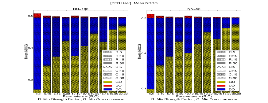
Fig. 1: This figure shows the mean NDCG per user, for 100 visual neighbors on the left, and 50 visual neighbors on the right. The performance is similar for both. Each bar on the x-axis corresponds to specific settings of the R and C parameters. The default ordering $DO$ is the baseline $XE$ [4]

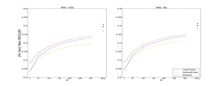
Fig. 2: This figure shows the mean NDCG@K per user, for 100 visual neighbors on the left, and 50 visual neighbors on the right. The performance is similar for both. The x-axis corresponds to K.

We also evaluate the performance of the global (or “average user”, yellow bar/line), pairwise preferences, and we see that enforcing pairwise orders based on a global/average notion of preference actually degrades the performance. Except for $K=1$, the $nDCG@K$ metric for the global preferences is worse than the baseline. This might be because, users tend to use more global/popular tags in the beginning of their ranked lists, so that we are actually able to learn with enough data, certain global biases among the popular tags. Beyond that, because users tag differently, enforcing a global preference is actually counterproductive. We also observe the reverse trend as we fix $C$ and vary $R$ (and vice-versa) to that of the personal preferences. This is because to estimate global preferences we need to observe a lot more data than for a single user, and so estimating for pairs without a lot of co-occurrences will invariably lead to over-fitting.

Figure 2, shows the $nDCG@K$ as $K$ varies under the best choices of parameters $R$ and $C$, for both the global and personal preferences. The best choices for the global were, $R=C=30$, and for the personal, $R=C=5$. We see, averaging over both users and images(included in the appendix), that the baseline outperforms the global (except at $K=1$), and the personal outperforms the baseline. These observations imply that picking lower parameters is usually better for the personal preferences, while higher values of $R$ and $C$ are necessary for the global preferences to be useful.

Table 1 shows that our method on average is $6\%$ better than the baseline method, and this improvement goes up to about $30\%$, for $nDCG@1$, as can be seen from Figure 2.

The above observations are true for both the average across all the images in our test set, and across all the users’ mean $nDCG$. This shows that the gains we get are relatively consistent for each user. This combined with the fact that the global pairwise preferences under-perform, imply that true personal pairwise preferences indeed exist, can be estimated, and can be used to improve the performance of automatic image tagging.

We include more detailed plots in the supplemntary appendix.

5 Conclusion

In this work we proposed a new measurement of tag preferences, and demonstrated that there is indeed a tag-order bias, that is, when a user mentions tag $a$ before tag $b$, in a list of tags for a given image, the user is implying that he prefers, or considers $a$ to be of greater importance than $b$. We showed that this bias can be learned from historical data using the maximum likelihood estimate based on a pair’s co-occurrence, and subsequently showed that such information can be exploited to improve the performance of current state-of-art automated image tagging systems.

We also defined a new tagging objective function that assumes the inherent pairwise bias between tags, and provided an algorithm which optimizes the new objective (under some mild conditions), and helped verify our claims and assumptions.

This leads us to conclude that although there are many visual factors that may affect what tags a user will provide for an image, it is useful to characterize instead (or rather in conjunction) the users’ tagging habits to learn what tags are of more importance to the users, whether they are visually motivated or not, and automatic tagging systems should employ this technique to improve their overall performance.

6 Future Work

We believe that there are several ways that this work could be extended or extend other works. One direction we see is working on algorithms that provide tight guarantees for solving our tagging objective, or even solves it optimally, even in the presence of dependent cycles. Another direction comes from the observation that most tag pairs never occur, but it may be possible to learn a function that maps a pair of tags to a real number indicating the direction and strength of the preference. It would also be interesting to see how the assumptions made in this paper can be used to extend the works on learning for personalized ranking [20, 21, 22]. We think it would also be interesting to explore the cognitive dimensions that drive tag ordering, and how these cognitive dimensions contribute to the tagging choices both independently and collectively.

References

- [1] Amandianeze O. Nwana and Tsuhan Chen, “Towards understanding user preferences from user tagging behavior,” CoRR, vol. abs/1507.05150, 2015.
- [2] “Flickr,” http://www.flickr.com, Last Accessed: 12/03/2015.
- [3] “On flickr ordering,” https://www.flickr.com/help/forum/en-us/72157645219834187/, Last Accessed: 12/03/2015.
- [4] Xirong Li, Efstratios Gavves, Cees G.M. Snoek, Marcel Worring, and Arnold W.M. Smeulders, “Personalizing automated image annotation using cross-entropy,” in Proceedings of the 19th ACM International Conference on Multimedia, New York, NY, USA, 2011, MM ’11, pp. 233–242, ACM.
- [5] Jason Weston, Samy Bengio, and Nicolas Usunier, “Wsabie: Scaling up to large vocabulary image annotation,” in Proceedings of the Twenty-Second International Joint Conference on Artificial Intelligence - Volume Volume Three. 2011, IJCAI’11, pp. 2764–2770, AAAI Press.
- [6] Stefanie Lindstaedt, Viktoria Pammer, Roland Mörzinger, Roman Kern, Helmut Mülner, and Claudia Wagner, “Recommending tags for pictures based on text, visual content and user context,” in Proceedings of the 2008 Third International Conference on Internet and Web Applications and Services, Washington, DC, USA, 2008, ICIW ’08, pp. 506–511, IEEE Computer Society.
- [7] Julian J. McAuley and Jure Leskovec, “Image labeling on a network: Using social-network metadata for image classification,” CoRR, vol. abs/1207.3809, 2012.
- [8] Neela Sawant, Ritendra Datta, Jia Li, and James Z. Wang, “Quest for relevant tags using local interaction networks and visual content,” in Proceedings of the International Conference on Multimedia Information Retrieval, New York, NY, USA, 2010, MIR ’10, pp. 231–240, ACM.
- [9] Börkur Sigurbjörnsson and Roelof van Zwol, “Flickr tag recommendation based on collective knowledge,” in Proceedings of the 17th International Conference on World Wide Web, New York, NY, USA, 2008, WWW ’08, pp. 327–336, ACM.
- [10] Z. Stone, T. Zickler, and T. Darrell, “Autotagging facebook: Social network context improves photo annotation,” in Computer Vision and Pattern Recognition Workshops, 2008. CVPRW ’08. IEEE Computer Society Conference on, 2008, pp. 1–8.
- [11] Fabiano Belém, Eder Martins, Tatiana Pontes, Jussara Almeida, and Marcos Gonçalves, “Associative tag recommendation exploiting multiple textual features,” in Proceedings of the 34th International ACM SIGIR Conference on Research and Development in Information Retrieval, New York, NY, USA, 2011, SIGIR ’11, pp. 1033–1042, ACM.
- [12] A.C. Berg, T.L. Berg, H. Daume, J. Dodge, A. Goyal, Xufeng Han, A. Mensch, M. Mitchell, A. Sood, K. Stratos, and K. Yamaguchi, “Understanding and predicting importance in images,” in Computer Vision and Pattern Recognition (CVPR), 2012 IEEE Conference on, June 2012, pp. 3562–3569.
- [13] Merrielle Spain and Pietro Perona, “Measuring and predicting object importance,” Int. J. Comput. Vision, vol. 91, no. 1, pp. 59–76, Jan. 2011.
- [14] Arnold W. M. Smeulders, Marcel Worring, Simone Santini, Amarnath Gupta, and Ramesh Jain, “Content-based image retrieval at the end of the early years,” IEEE TRANSACTIONS ON PATTERN ANALYSIS AND MACHINE INTELLIGENCE, vol. 22, no. 12, pp. 1349–1380, 2000.
- [15] A. Th. (Guus) Schreiber, Barbara Dubbeldam, Jan Wielemaker, and Bob Wielinga, “Ontology-based photo annotation,” 2001.
- [16] Tye Rattenbury, Nathaniel Good, and Mor Naaman, “Towards automatic extraction of event and place semantics from flickr tags,” in Proceedings of the 30th Annual International ACM SIGIR Conference on Research and Development in Information Retrieval, New York, NY, USA, 2007, SIGIR ’07, pp. 103–110, ACM.
- [17] Patrick Schmitz, “Inducing ontology from flickr tags,” in Proceedings of the Workshop on Collaborative Tagging at WWW2006, Edinburgh, Scotland, May 2006.
- [18] Gediminas Adomavicius, Ramesh Sankaranarayanan, Shahana Sen, and Alexander Tuzhilin, “Incorporating contextual information in recommender systems using a multidimensional approach,” ACM Trans. Inf. Syst., vol. 23, no. 1, pp. 103–145, Jan. 2005.
- [19] Yehuda Koren, Robert Bell, and Chris Volinsky, “Matrix factorization techniques for recommender systems,” Computer, vol. 42, no. 8, pp. 30–37, Aug. 2009.
- [20] Steffen Rendle, Christoph Freudenthaler, Zeno Gantner, and Lars Schmidt-Thieme, “Bpr: Bayesian personalized ranking from implicit feedback,” in Proceedings of the Twenty-Fifth Conference on Uncertainty in Artificial Intelligence, Arlington, Virginia, United States, 2009, UAI ’09, pp. 452–461, AUAI Press.
- [21] Steffen Rendle and Lars Schmidt-Thieme, “Pairwise interaction tensor factorization for personalized tag recommendation,” in Proceedings of the Third ACM International Conference on Web Search and Data Mining, New York, NY, USA, 2010, WSDM ’10, pp. 81–90, ACM.
- [22] Weike Pan and Li Chen, “Gbpr: Group preference based bayesian personalized ranking for one-class collaborative filtering,” in Proceedings of the Twenty-Third International Joint Conference on Artificial Intelligence. 2013, IJCAI ’13, pp. 2691–2697, AAAI Press.
- [23] Shi Peng, Qu Yunqing, and Liang Hongshuo, “Personalized image tag recommendation algorithm for web2.0 platform utilizing tensor factorization,” in Proceedings of the 2014 Fifth International Conference on Intelligent Systems Design and Engineering Applications, Washington, DC, USA, 2014, ISDEA ’14, pp. 718–721, IEEE Computer Society.
- [24] Nachiketa Sahoo, Ramayya Krishnan, George Duncan, and Jamie Callan, “The halo effect in multicomponent ratings and its implications for recommender systems: The case of yahoo! movies,” Information Systems Research, vol. 23, no. 1, pp. 231–246, 2012.
- [25] Shilad Sen, Jesse Vig, and John Riedl, “Tagommenders: Connecting users to items through tags,” in Proceedings of the 18th International Conference on World Wide Web, New York, NY, USA, 2009, WWW ’09, pp. 671–680, ACM.
- [26] Yang Song, Ziming Zhuang, Huajing Li, Qiankun Zhao, Jia Li, Wang-Chien Lee, and C. Lee Giles, “Real-time automatic tag recommendation,” in Proceedings of the 31st Annual International ACM SIGIR Conference on Research and Development in Information Retrieval, New York, NY, USA, 2008, SIGIR ’08, pp. 515–522, ACM.
- [27] Thomas H. Cormen, Charles E. Leiserson, Ronald L. Rivest, and Clifford Stein, MIT Press and McGraw-Hill, 2001.
- [28] Tat-Seng Chua, Jinhui Tang, Richang Hong, Haojie Li, Zhiping Luo, and Yan-Tao. Zheng, “Nus-wide: A real-world web image database from national university of singapore,” in Proc. of ACM Conf. on Image and Video Retrieval (CIVR’09), Santorini, Greece., July 8-10, 2009.
- [29] David G. Lowe, “Distinctive image features from scale-invariant keypoints,” Int. J. Comput. Vision, vol. 60, no. 2, pp. 91–110, Nov. 2004.
- [30] Xirong Li, Cees G. M. Snoek, and Marcel Worring, “Unsupervised multi-feature tag relevance learning for social image retrieval,” in Proceedings of the ACM International Conference on Image and Video Retrieval, New York, NY, USA, 2010, CIVR ’10, pp. 10–17, ACM.