Smooth quantum gravity: Exotic smoothness and Quantum gravity

Abstract

Over the last two decades, many unexpected relations between exotic smoothness, e.g. exotic $\mathbb{R}^{4}$, and quantum field theory were found. Some of these relations are rooted in a relation to superstring theory and quantum gravity. Therefore one would expect that exotic smoothness is directly related to the quantization of general relativity. In this article we will support this conjecture and develop a new approach to quantum gravity called smooth quantum gravity by using smooth 4-manifolds with an exotic smoothness structure. In particular we discuss the appearance of a wildly embedded 3-manifold which we identify with a quantum state. Furthermore, we analyze this quantum state by using foliation theory and relate it to an element in an operator algebra. Then we describe a set of geometric, non-commutative operators, the skein algebra, which can be used to determine the geometry of a 3-manifold. This operator algebra can be understood as a deformation quantization of the classical Poisson algebra of observables given by holonomies. The structure of this operator algebra induces an action by using the quantized calculus of Connes. The scaling behavior of this action is analyzed to obtain the classical theory of General Relativity (GRT) for large scales. This approach has some obvious properties: there are non-linear gravitons, a connection to lattice gauge field theory and a dimensional reduction from 4D to 2D. Some cosmological consequences like the appearance of an inflationary phase are also discussed. At the end we will get the simple picture that the change from the standard $\mathbb{R}^{4}$ to the exotic $R^{4}$ is a quantization of geometry.

On the occasion of the 80-th birthday of Carl H. Brans

1 Introduction

On the 25-th of November in 1915, Einstein presented his field equations, the basic equations of General Relativity, to the Prussian Academy of Sciences in Berlin. This equation had a tremendous impact on physics, in particular on cosmology. The essence of the theory was expressed by Wheeler by the words: Spacetime tells matter how to move; matter tells spacetime how to curve. Einsteins theory remained unchanged for about 40 years. Then one started to investigate theories fulfilling Mach’s principle leading to a variable gravitational constant. Brans-Dicke theory was the first realization of an extended Einstein theory with variable gravitational constant (Jordans proposal was not widely known). All experiments are, however, in good agreement with Einstein’s theory and currently there is no demand to change it.

General relativity (GR) has changed our understanding of space-time. In parallel, the appearance of quantum field theory (QFT) has modified our view of particles, fields and the measurement process. The usual approach for the unification of QFT and GR to a quantum gravity, starts with a proposal to quantize GR and its underlying structure, space-time. There is a unique opinion in the community about the relation between geometry and quantum theory: The geometry as used in GR is classical and should emerge from a quantum gravity in the limit (Planck’s constant tends to zero). Most theories went a step further and try to get a space-time from quantum theory. Then, the model of a smooth manifold is not suitable to describe quantum gravity, but there is no sign for a discrete space-time structure or higher dimensions in current experiments [41]. Therefore, we conjecture that the model of spacetime as a smooth 4-manifold can be used also in a quantum gravity regime, but then one has the problem to represent QFT by geometric methods (submanifolds for particles or fields etc.) as well to quantize GR. In particular, one must give meaning to the quantum state by geometric methods. Then one is able to construct the quantum theory without quantization. Here we implicitly assumed that the quantum state is real, i.e. the quantum state or the wave function has a real counterpart and is not a collection of future possibilities representing some observables. Experiments [75, 28, 83] supported this view. Then the wave function is not merely representing our limited knowledge of a system but it is in direct correspondence to reality! Then one has to go the reverse way: one has to show that the quantum state is produced by the quantization of a classical state. It is, however, not enough to have a geometric approach to quantum gravity (or the quantum field theory in general). What are the quantum fluctuations? What is the measurement process? What is decoherence and entanglement? In principle, all these questions have to be addressed too.

Here, the exotic smoothness structure of 4-manifolds can help finding a way. A lot of work was done in the last decades to fulfill this goal. It starts with the work of Brans and Randall [32] and of Brans alone [29, 30, 31] where the special situation in exotic 4-manifolds (in particular the exotic $\mathbb{R}^{4}$) was explained. One main result of this time was the Brans conjecture: exotic smoothness can serve as an additional source of gravity. I will not present the whole history where I refer to Carl’s article. Here I will list only some key results which will be used in the following

• Exotic smoothness is an extra source of gravity (Brans conjecture is true), see Asselmeyer [5] for compact manifolds and Sładkowski [86, 87] for the exotic $\mathbb{R}^{4}$. Therefore an exotic $\mathbb{R}^{4}$ is always curved and cannot be flat!

• The exotic $\mathbb{R}^{4}$ cannot be a globally hyperbolic space (see [40] for instance), i.e. represented by $M\times\mathbb{R}$ for some 3-manifold. Instead it admits complicated foliations [17]. Using non-commutative geometry, we are able to study these foliations (the leaf space) and get relations to QFT. For instance, the von Neumann algebra of a codimension-one foliation of an exotic $\mathbb{R}^{4}$ must contain a factor of type $I\!I\!I_{1}$ used in local algebraic QFT to describe the vacuum [11, 13, 19].

• The end of $\mathbb{R}^{4}$ (the part extending to infinity) is $S^{3}\times\mathbb{R}$. If $\mathbb{R}^{4}$ is exotic then $S^{3}\times\mathbb{R}$ admits also an exotic smoothness structure. Clearly, there is always a topologically embedded 3-sphere but there is no smoothly embedded one. Let us assume the well-known hyperbolic metric of the spacetime $S^{3}\times\mathbb{R}$ using the trivial foliation into leafs $S^{3}\times\left\{t\right\}$ for all $t\in\mathbb{R}$. Now we demand that $S^{3}\times\mathbb{R}$ carries an exotic smoothness structure at the same time. Then we will get only topologically embedded 3-spheres, the leafs $S^{3}\times\left\{t\right\}$. These topologically embedded 3-spheres are also known as wild 3-spheres. In [14], we presented a relation to quantum D-branes. Finally we proved in [16] that the deformation quantization of a tame embedding (the usual embedding) is a wild embedding. Furthermore we obtained a geometric interpretation of quantum states: wild embedded submanifolds are quantum states. Importantly, this construction depends essentially on the continuum, because wild embedded submanifolds admit always infinite triangulations.

• For a special class of compact 4-manifolds we showed in [20] that exotic smoothness can generate fermions and gauge fields using the so-called knot surgery of Fintushel and Stern [51]. In the paper [10] we presented an approach using the exotic $\mathbb{R}^{4}$ where the matter can be generated (like in QFT).

• The path integral in quantum gravity is dominated by the exotic smoothness contribution (see [6, 50, 80] or by using string theory [12]).

The paper is organized as follows. In the following three sections we will explain exotic 4-manifolds and motivate the whole approach by using the path integral for the Einstein-Hilbert action. Here we will also present how to couple the matter and gauge fields to this theory. For a 4-manifold, there are two main invariants the Euler and Pontrjagin class which determine the main topological invariant of a 4-manifold, the intersection form. In section 5, we will obtain the Einstein-Hilbert and Holst action by using these two classes. At the first view, this section is a little bit isolated from the previous and subsequent sections but we will use this result later during the study of the scaling. In the main section 6, we will construct the foliation of an exotic $\mathbb{R}^{4}$ of codimension (equivalent to a Lorentz structure). Following Connes, [42] the leaf space is an operator algebra constructed from the geometrical information of the foliation (holonomy groupoid). This operator algebra is a factor $I\!I\!I$ von Neumann algebra and we will use the Tomita-Takesaki modular theory to uncover the structure of the foliation. It is not the first time that this factor was used for quantum gravity and we refer to the paper [22] for a nice application. States in this operator algebra are represented by equivalence classes of knotted curves (element of the Kauffman bracket skein module). The reconstruction of the spatial space from the states gives a wild embedded 3-sphere as geometrical representation of the state. Surprisingly, it fits with the properties of the exotic $\mathbb{R}^{4}$. If one introduces a global foliation of the exotic $\mathbb{R}^{4}$ by a global time then one obtains a foliation into wild embedded 3-spheres. In contrast, if one uses a local but complicate foliation then this wild object can be omitted and one obtains a state given by a finite collection of knotted curves. Interestingly, the operator algebra can be understood as observable algebra given by a deformation quantization (Turaev-Drinfeld quantization [97, 98]) of the classical observable algebra (Poisson algebra of holonomies a la Goldman [61]). In section 7, we will use the splitting of the operator algebra (10) given by Tomita-Takesaki modular theory to introduce the dynamics (see Connes and Rovelli [44] with similar ideas). Finally we will obtain a quantum action (15) in the quantized calculus of Connes [43]. Then the scaling behavior is studied in the next section. For large scales, the action can be interpreted as a non-linear sigma model. The renormalization group (RG) flow analysis [56] gives the Einstein equations for large scales. The short-scale analysis is much more involved, yielding for small fluctuations the Einstein-Hilbert action and a non-minimally coupled scalar field. In particular, we will obtain a $(2+\epsilon)-$dimensional fractal structure. In section 9 we will present some direct consequences of this approach: the nonlinear graviton [79], a relation to lattice gauge field theory with a discussion of discreteness and the appearance of dimensional reduction from 4D to 2D. In section 10 we will discuss the answer to a fundamental question: where does the quantum fluctuations come from? The main result of this section can be written as: The set of canonical pairs (as measurable variables in the theory) forms a fractal subset of the space of all holonomies. Then we can only determine the initial condition up to discrete value (given by the canonical pair) and the chaotic behavior of the foliation (i.e. the Anosov flow) makes the limit not predictable. This interesting result is followed by a section where we will discuss the collapse of the wavefunction by the gravitational interaction by calculating the minimal decoherence time. Furthermore we will discuss entanglement and the measurement process. In section 12 we will list our work in cosmology which uses partly the results of this paper. In the last section 13, we will discuss some consequences and open questions. Some mathematical prerequisites are presented in three appendices.

This article is dedicated to my only teacher, Carl H. Brans for 20 years of collaboration and friendship. He is the founder of this research area. We had and will have many interesting discussions. Carl always asked the right question and put the finger on many open points. During the 7 years of writing our book, we had a very fruitful collaboration and I learned so much to complete even this work. Carl, I hope for many discussions with you in the future. I’m very glad to count on your advice. Happy Birthday!

2 What is Exotic Smoothness?

Why am I going to concentrate on a concept like exotic smoothness? Einstein used the equivalence principle as a key principle in the development of general relativity. Every gravitational field can be locally eliminated by acceleration. Then, the spacetime is locally modeled as subsets of the flat $\mathbb{R}^{4}$ or the equivalence principle enforces us to use the concept of a manifold for spacetime. Together with the smoothness of the dynamics (usage of differential equations), we obtain a smooth 4-manifold as model for the spacetime in agreement with the current experimental situation. A manifold consists of charts and transition functions forming an atlas which covers the manifold completely. The smooth atlas is called the smoothness structure of the manifold. It was an open problem for a long time whether every topological manifold admits a unique smooth atlas. In 1957, Milnor found the first counterexample: the construction of a 7-sphere with at least 8 different smoothness structures. Later it was shown that all manifolds of dimension larger than 4 admit only a finite number of distinct smoothness structures. The real breakthrough for 4-manifolds came in the 80’s where one constructed infinitely many different smoothness structures for many compact 4-manifolds (countably infinite) and for many non-compact 4-manifolds (uncountably infinite) including the $\mathbb{R}^{4}$. In all dimensions smaller than four, there is only one smoothness structure (up to diffeomorphisms), the standard structure. The standard $\mathbb{R}^{4}$ is simply characterized by the unique property to split smoothly like $\mathbb{R}^{4}=\mathbb{R}\times\mathbb{R}\times\mathbb{R}\times\mathbb{R}$. All other distinct smoothness structures are called exotic smoothness structures. These structures are different, nonequivalent, smooth descriptions of the same topological manifold, a different atlas of charts. In case of the exotic $\mathbb{R}^{4}$, the difference is tremendous: the standard $\mathbb{R}^{4}$ needs one chart (and every other description can be reduced to it) whereas every known exotic $\mathbb{R}^{4}$ admits infinitely many charts (which cannot be reduced to a simpler description). So, the spacetime exhibits a much larger complexity by using an exotic smoothness structure, but why is dimension 4 so special? There is a good description in [55] and I will give a short account now. At first we have to discuss the question: how do I build an atlas for a smooth manifold? The answer is given by considering the construction of diffeomorphisms. Every diffeomorphism is locally given by the solution of $\dot{\vec{x}}=-\nabla f(\vec{x})$ for a real function $f$ over the manifold. The fixed points of this equation are the critical points of $f$. In case of isolated critical points, one can reproduce the structure of the manifold (this is called Morse theory). Every critical point leads to the attachment of a handle, a submanifold like $D^{n-k}\times D^{k}$, i.e. the $k-$handle (where $D^{k}$ is the $k-$disk). In many cases, the corresponding structure of the manifold, the handle body, can be very complicated but there are rules (handle sliding) to simplify them. In all dimensions except dimension 4. Therefore, two handle bodies can be described by the same 4-manifold topologically but differ in the smooth description.

3 The Main Example: Exotic $\mathbb{R}^{4}$

One of the most surprising aspects of exotic smoothness is the existence of exotic $\mathbb{R}^{4}$’s. In all other dimensions [88], the Euclidean space $\mathbb{R}^{n}$ with $n\not=4$ admits a unique smoothness structure, up to diffeomorphisms. Beginning with the first examples [66], Taubes [93] and Freedman/DeMichelis [47] constructed countably many large and small exotic $\mathbb{R}^{4}$’s, respectively. A small exotic $\mathbb{R}^{4}$ embeds smoothly in the 4-sphere whereas a large exotic $\mathbb{R}^{4}$ cannot be embedded in that way. For the following we need some simple definitions: the connected sum $\#$ and the boundary connected sum $\natural$ of manifolds. Let $M,N$ be two $n$-manifolds with boundaries $\partial M,\partial N$. The connected sum $M\#N$ is the procedure of cutting out a disk $D^{n}$ from the interior $int(M)\setminus D^{n}$ and $int(N)\setminus D^{n}$ with the boundaries $S^{n-1}\sqcup\partial M$ and $S^{n-1}\sqcup\partial N$, respectively, and gluing them together along the common boundary component $S^{n-1}$. The boundary $\partial(M\#N)=\partial M\sqcup\partial N$ is the disjoint sum of the boundaries $\partial M,\partial N$. The boundary connected sum $M\natural N$ is the procedure of cutting out a disk $D^{n-1}$ from the boundary $\partial M\setminus D^{n-1}$ and $\partial N\setminus D^{n-1}$ and gluing them together along $S^{n-2}$ of the boundary. Then the boundary of this sum $M\natural N$ is the connected sum $\partial(M\natural N)=\partial M\#\partial N$ of the boundaries $\partial M,\partial N$.

3.1 Large Exotic $\mathbb{R}^{4}$

Large exotic $\mathbb{R}^{4}$ can be constructed using the failure to arbitrarily split a compact, simply-connected 4-manifold. For every topological 4-manifold one knows how to split this manifold topologically into simpler pieces using the work of Freedman [53]. Donaldson [48], however, that some of these 4-manifolds do not exist as smooth 4-manifolds. This contradiction between the continuous and the smooth case produces the first examples of exotic $\mathbb{R}^{4}$. Below we discuss one of these examples.

One starts with a compact, simply-connected 4-manifold $X$ classified by the intersection form [53]

$$Q_{X}:H_{2}(X,\mathbb{Z})\times H_{2}(X,\mathbb{Z})\to\mathbb{Z}$$

a quadratic form over the second integer homology group. In the first construction of a large exotic $\mathbb{R}^{4}$, one starts with the K3 surface as 4-manifold having the intersection form

$$Q_{K3}=E_{8}\oplus E_{8}\oplus(\oplus_{3}\left(\begin{array}[]{cc}0&1\\ 1&0\end{array}\right)):=2E_{8}\oplus 3H$$ (1)

with the the matrix $E_{8}$:

$$E_{8}=\left[\begin{array}[]{cccccccc}2&1&0&0&0&0&0&0\\ 1&2&1&0&0&0&0&0\\ 0&1&2&1&0&0&0&0\\ 0&0&1&2&1&0&0&0\\ 0&0&0&1&2&1&0&1\\ 0&0&0&0&1&2&1&0\\ 0&0&0&0&0&1&2&0\\ 0&0&0&0&1&0&0&2\end{array}\right].$$

The work of Donaldson [48] shows that a closed, smooth, simply-connected, compact 4-manifold $X_{E_{8}\oplus E_{8}}$ with intersection form $E_{8}\oplus E_{8}$ does not exist. Freedman [53] showed, however, that there is a topological splitting

$$K3=X_{E_{8}\oplus E_{8}}\#\left(\#_{3}(S^{2}\times S^{2})\right)$$ (2)

with the $m-$times connected sum $\#_{m}$ (see above) which fails to be smooth. This splitting means that we glue together the two manifolds $\#_{3}(S^{2}\times S^{2})\setminus D^{4}$ and $X_{E_{8}\oplus E_{8}}\setminus D^{4}$ along the common boundary $S^{3}=\partial D^{4}$ ($D^{4}$ is the 4-disk or 4-ball). Now we define the interior $X=\#_{3}(S^{2}\times S^{2})\setminus Int\,D^{4}$. The splitting (2) gives a way to represent the $3H$ part of the intersection form (1) by using $X$ but that fails smoothly. So, choosing a topological splitting

$$K3 = X_{E_{8}\oplus E_{8}}\#\left(\#_{3}(S^{2}\times S^{2})\right)$$

$$= \left(X_{E_{8}\oplus E_{8}}\setminus D^{4}\right)\cup\left(S^{3}\times[0,1]\right)\cup\left(\#_{3}(S^{2}\times S^{2})\setminus D^{4}\right)$$

gives a $S^{3}\times[0,1]$ inside the $K3$. The interior of $S^{3}\times[0,1]$ defines a manifold $S^{3}\times[0,1)$ glued to a (topological) 4-disk $D^{4}\subset\#_{3}(S^{2}\times S^{2})\setminus D^{4}$ along the common boundary, i.e. $W=D^{4}\cup S^{3}\times[0,1)$ topologically. $W$ is homeomorphic to $\mathbb{R}^{4}$ but the non-existence of the smooth splitting implies that it is an exotic $\mathbb{R}^{4}$ and there is no smooth embedded $S^{3}$ (otherwise the topological splitting is smooth). This failure for a smooth embedding implies also that such exotic $\mathbb{R}^{4}$’s do not embed in the 4-sphere, i.e. it is a large exotic $\mathbb{R}^{4}$. The details of the construction can be found in our book [8] (section 8.4).

Gompf [64] introduced an important tool for finding new exotic ${{\mathbb{R}}^{4}}$ from others, the end-sum $\natural_{e}$. Let $R,R^{\prime}$ be two topological ${{\mathbb{R}}^{4}}$’s. The end-sum $R\natural_{e}R^{\prime}$ is defined as follows: Let $\gamma:[0,\infty)\to R$ and $\gamma^{\prime}:[0,\infty)\to R^{\prime}$ be smooth properly embedded rays with tubular neighborhoods $\nu\subset R$ and $\nu^{\prime}\subset R^{\prime}$, respectively. For convenience, identify the two semi-infinite intervals with $[0,1/2),$ and $(1/2,1]$ leading to diffeomorphisms, $\phi:\nu\to[0,1/2)\times\mathbb{R}^{3}$ and $\phi^{\prime}:\nu^{\prime}\to(1/2,1]\times\mathbb{R}^{3}$. Then define

$$R\natural_{e}R^{\prime}=R\cup_{\phi}I\times{\mathbb{R}}^{3}\cup_{\phi^{\prime}}R^{\prime}$$

as the end sum of $R$ and $R^{\prime}$. With a little checking, it is easy to see that this construction leads to $R\natural_{e}R^{\prime}$ as another topological $\mathbb{R}^{4}.$ However, if $R,R^{\prime}$ are themselves exotic, then so will $R\natural_{e}R^{\prime}$ and in fact, it will be a “new” exotic manifold, since it will not be diffeomorphic to either $R$ or $R^{\prime}$. Gompf used this technique to construct a class of exotic ${{\mathbb{R}}^{4}}$’s none of which can be embedded smoothly in the standard ${{\mathbb{R}}^{4}}$.

By an extension of Donaldson theory for a special class of open 4-manifolds, so-called end-periodic 4-manifolds, Taubes [93] gives a continuous family of exotic $\mathbb{R}^{4}$ which was extended by Gompf to a continuous 2-parameter family $R_{s,t}$.

3.2 Small Exotic $\mathbb{R}^{4}$

Small exotic $\mathbb{R}^{4}$’s are again the result of anomalous smoothness in 4-dimensional topology but of a different kind than for large exotic $\mathbb{R}^{4}$’s. In 4-manifold topology [53], a homotopy-equivalence between two compact, closed, simply-connected 4-manifolds implies a homeomorphism between them (a so-called h cobordism), but Donaldson [49] provided the first smooth counterexample, i.e. both manifolds are generally not diffeomorphic to each other. The failure can be localized in some contractible submanifold (Akbulut cork) so that an open neighborhood of this submanifold is a small exotic $\mathbb{R}^{4}$. The whole procedure implies that this exotic $\mathbb{R}^{4}$ can be embedded in the 4-sphere $S^{4}$. Below we discuss the details for one of these examples.

In 1975 Casson (Lecture 3 in [39]) described a smooth 5-dimensional h-cobordism between compact 4-manifolds and showed that they “differ” by two proper homotopy ${{\mathbb{R}}^{4}}$’s (see below). Freedman knew, as an application of his proper h-cobordism theorem, that the proper homotopy ${{\mathbb{R}}^{4}}$’s were ${{\mathbb{R}}^{4}}$. After hearing about Donaldson’s work in March 1983, Freedman realized that there should be exotic ${{\mathbb{R}}^{4}}$’s and, to find one, he produced the second part of the construction below involving the smooth embedding of the proper homotopy ${{\mathbb{R}}^{4}}$’s in $S^{4}$. Unfortunately, it was necessary to have a compact counterexample to the smooth h-cobordism conjecture, and Donaldson did not provide this until 1985 [49]. The idea of the construction is simply given by the fact that every such smooth h-cobordism between non-diffeomorphic 4-manifolds can be written as a product cobordism except for a compact contractible sub-h-cobordism $V$, the Akbulut cork. An open subset $U\subset V$ homeomorphic to $[0,1]\times{{\mathbb{R}}^{4}}$ is the corresponding sub-h-cobordism between two exotic ${{\mathbb{R}}^{4}}$’s. These exotic ${{\mathbb{R}}^{4}}$’s are called ribbon ${{\mathbb{R}}^{4}}$’s. They have the important property of being diffeomorphic to open subsets of the standard ${{\mathbb{R}}^{4}}$. That stands in contrast to the previous defined examples of Kirby, Gompf and Taubes.

To be more precise, consider a pair $(X_{+},X_{-})$ of homeomorphic, smooth, closed, simply-connected 4-manifolds. The transformation from $X_{-}$ to $X_{+}$ visualized by a h-cobordism can be described by the following construction.
Let $W$ be a smooth h-cobordism between closed, simply connected 4-manifolds $X_{-}$ and $X_{+}$. Then there is an open subset $U\subset W$ homeomorphic to $[0,1]\times{{\mathbb{R}}^{4}}$ with a compact subset $K\subset U$ such that the pair $(W\setminus K,U\setminus K)$ is diffeomorphic to a product $[0,1]\times(X_{-}\setminus K,U\cap X_{-}\setminus K)$. The subsets $R_{\pm}=U\cap X_{\pm}$ (homeomorphic to ${{\mathbb{R}}^{4}}$) are diffeomorphic to open subsets of ${{\mathbb{R}}^{4}}$. If $X_{-}$ and $X_{+}$ are not diffeomorphic, then there is no smooth 4-ball in $R_{\pm}$ containing the compact set $Y_{\pm}=K\cap R_{\pm}$, so both $R_{\pm}$ are exotic ${{\mathbb{R}}^{4}}$’s.
Thus, remove a certain contractible, smooth, compact 4-manifold $Y_{-}\subset X_{-}$ (called an Akbulut cork) from $X_{-}$, and re-glue it by an involution of $\partial Y_{-}$, i.e. a diffeomorphism $\tau:\partial Y_{-}\to\partial Y_{-}$ with $\tau\circ\tau=Id$ and $\tau(p)\not=\pm p$ for all $p\in\partial Y_{-}$. This argument was modified above so that it works for a contractible open subset $R_{-}\subset X_{-}$ with similar properties, such that $R_{-}$ will be an exotic ${{\mathbb{R}}^{4}}$ if $X_{+}$ is not diffeomorphic to $X_{-}$. Furthermore $R_{-}$ lies in a compact set, i.e. a 4-sphere or $R_{-}$ is a small exotic $\mathbb{R}^{4}$. In the next subsection we will see how this results in the construction of handle bodies of exotic ${{\mathbb{R}}^{4}}$. In [47] Freedman and DeMichelis constructed also a continuous family of small exotic $\mathbb{R}^{4}$.

3.3 Main Property of (Small) Exotic $\mathbb{R}^{4}$

One of the characterizing properties of an exotic $\mathbb{R}^{4}$ (all known examples) is the existence of a compact subset $K\subset R^{4}$ which cannot be surrounded by any smoothly embedded 3-sphere (and homology 3-sphere bounding a contractible, smooth 4-manifold). Let $\mathbf{R}^{4}$ be the standard $\mathbb{R}^{4}$ (i.e. $\mathbf{R}^{4}=\mathbb{R}^{3}\times\mathbb{R}$ smoothly) and let $R^{4}$ be a small exotic $\mathbb{R}^{4}$ with compact subset $K\subset R^{4}$ which cannot be surrounded by a smoothly embedded 3-sphere. Then every completion $\overline{N(K)}$ of an open neighborhood $N(K)\subset R^{4}$ is not bounded by a 3-sphere $S^{3}\not=\partial\overline{N(K)}$. However, $R^{4}$ is a small exotic $\mathbb{R}^{4}$ and there is a smooth embedding $E:R^{4}\to\mathbf{R}^{4}$ in the standard $\mathbb{R}^{4}$. Then the completion of the image $\overline{E(R^{4})}$ has the boundary $S^{3}=\partial\overline{E(R^{4})}$ as subset of $\mathbf{R}^{4}$. So, we have the strange situation that an open subset of the standard $\mathbf{R}^{4}$ represents a small exotic $R^{4}$. In case of the large exotic $\mathbb{R}^{4}$, the situation is much more complicated. A large exotic $\mathbb{R}^{4}$ does not embed in any smooth 4-manifold which is simpler than the manifold used for the construction of this exotic $\mathbb{R}^{4}$. Above we considered the example of a large exotic $\mathbb{R}^{4}$ constructed from a K3 surface. Therefore this large exotic $\mathbb{R}^{4}$ embeds in the K3 surface but not in simpler 4-manifolds like $\mathbb{C}P^{2}$.

3.4 Handle decomposition of the small exotic $\mathbb{R}^{4}$ and Casson handles

As of now, we only know of exotic $\mathbb{R}^{4}$’s represented by an infinite number of coordinate patches. This naturally makes it difficult to provide an explicit description of a metric. However, in [9], a suggestion to overcome this limitation is provided by the consideration of periodic explicitly described coordinate patches making use of more complex pieces, so-called handles, and even more complex gluing maps. Then one also gets infinite structures of handles but with a clear picture: the coordinate patches have a periodic structure.

Handles Every 4-manifold can be decomposed using standard pieces such as $D^{k}\times D^{4-k}$, the so-called $k$-handle attached along $\partial D^{k}\times D^{4-k}$ to the $0-$handle $D^{0}\times D^{4}=D^{4}$. In the following we need two possible cases: the 1-handle $D^{1}\times D^{3}$ and the 2-handle $D^{2}\times D^{2}$. These handles are attached along their boundary components $S^{0}\times D^{3}$ or $S^{1}\times D^{2}$ to the boundary $S^{3}$ of the $0-$handle $D^{4}$ (see [68] for the details). The attachment of a 2-handle is defined by a map $S^{1}\times D^{2}\to S^{3}$, the embedding of a circle $S^{1}$ into the 3-sphere $S^{3}$, i.e. a knot. This knot into $S^{3}$ can be thickened (to get a knotted solid torus). The important fact for our purposes is the freedom to twist this knotted solid torus (so-called Dehn twist). The (integer) number of these twists (with respect to the orientation) is called the framing number or the framing. Thus the gluing of the 2-handle on $D^{4}$ can be represented by a knot or link together with an integer framing. The simplest example is the unknot with framing $\pm 1$ representing the complex projective space $\mathbb{C}P^{2}$ or with reversed orientation $\overline{\mathbb{C}P}^{2}$, respectively. The 1-handle will be glued by the map of $S^{0}\times D^{3}\to S^{3}$ represented by two disjoint solid 2-spheres $D^{3}$. Akbulut [2] introduced another description. He observed that a 1-handle is something like a cut-out 2-handle with a fixed framing. We remark that all details can be found in [68]. Now we are ready to discuss the handle body decomposition of an exotic $\mathbb{R}^{4}$ by Bizaca and Gompf [24].

Handle decomposition of small exotic $\mathbb{R}^{4}$ First it is very important to notice that the exotic $\mathbb{R}^{4}$ is the interior of the handle body described below (since the handle body has a non-null boundary and is compact). The construction of the handle body can be divided into two parts. The first part is a submanifold consisting of a pair of a 1- and a 2-handle. This pair can be canceled topologically by using a Casson handle and we obtain the topological 4-disk $D^{4}$ with $\mathbb{R}^{4}$ as interior. This submanifold is a smooth 4-manifold with a boundary that can be covered by a finite number of charts. The smoothness structure of the exotic $\mathbb{R}^{4}$, however, depends mainly on the infinite Casson handle.

Casson handle Now consider the Casson handle and its construction in more detail. Briefly, a Casson handle $CH$ is the result of attempts to embed a disk $D^{2}$ into a 4-manifold. In most cases this attempt fails and Casson [39] looked for a substitute, which is now called a Casson handle. Freedman [53] showed that every Casson handle $CH$ is homeomorphic to the open 2-handle $D^{2}\times\mathbb{R}^{2}$ but in nearly all cases it is not diffeomorphic to the standard handle [63, 65]. The Casson handle is built by iteration, starting from an immersed disk in some 4-manifold $M$, i.e. an injective smooth map $D^{2}\to M.$ Every immersion $D^{2}\to M$ is an embedding except on a countable set of points, the double points. One can kill one double point by immersing another disk into that point. These disks form the first stage of the Casson handle. By iteration one can produce the other stages. Finally consider not the immersed disk but rather a tubular neighborhood $D^{2}\times D^{2}$ of the immersed disk including each stage. The union of all neighborhoods of all stages is the Casson handle $CH$. So, there are two input data involved with the construction of a $CH$: the number of double points in each stage and their orientation $\pm$. Thus we can visualize the Casson handle $CH$ by a tree: the root is the immersion $D^{2}\to M$ with $k$ double points, the first stage forms the next level of the tree with $k$ vertices connected with the root by edges etc. The edges are evaluated using the orientation $\pm$. Every Casson handle can be represented by such an infinite tree. The Casson handle $CH(R_{+})$ having an immersed disk with one (positively oriented) self-intersection (or double point) is the simplest Casson handle represented by the simplest tree $T_{+}$ having one vertex in each level connected by one edge with evaluation $+$.

3.5 Small Exotic $\mathbb{R}^{4}$ as a Sequence of 3-Manifolds

One of the characterizing properties of an exotic $\mathbb{R}^{4}$ (all known examples) is the existence of a compact subset $K\subset R^{4}$ which cannot be surrounded by any smoothly embedded 3-sphere (and homology 3-sphere bounding a contractible, smooth 4-manifold). Let $\mathbf{R}^{4}$ be the standard $\mathbb{R}^{4}$ (i.e. $\mathbf{R}^{4}=\mathbb{R}^{3}\times\mathbb{R}$ smoothly) and let $R^{4}$ be a small exotic $\mathbb{R}^{4}$ with compact subset $K\subset R^{4}$ which cannot be surrounded by a smoothly embedded 3-sphere. Then every completion $\overline{N(K)}$ of an open neighborhood $N(K)\subset R^{4}$ is not bounded by a 3-sphere $S^{3}\not=\partial\overline{N(K)}$, but $R^{4}$ is a small exotic $\mathbb{R}^{4}$ and there is a smooth embedding $E:R^{4}\to\mathbf{R}^{4}$ in the standard $\mathbb{R}^{4}$. Then the completion of the image $\overline{E(R^{4})}$ has the boundary $S^{3}=\partial\overline{E(R^{4})}$ as subset of $\mathbf{R}^{4}$. So, we have the strange situation that an open subset of the standard $\mathbf{R}^{4}$ represents a small exotic $R^{4}$.

Now we will describe $R^{4}$. Historically it was constructed by using a counterexample of the smooth h-cobordism theorem [49, 24]. Then the compact subset $K$ is given by a non-canceling 1-/2-handle pair. The attachment of a Casson handle $CH$ cancels this pair topologically. Then one obtains the 4-disk $D^{4}$ with interior $\mathbf{R}^{4}$, but this cancellation of the 1/2-handle pair cannot be done smoothly and one obtains a small exotic $R^{4}$ which is schematically given by $R^{4}=K\cup CH$. Remember $R^{4}$ is a small exotic $\mathbb{R}^{4}$, i.e. $R^{4}$ is embedded into the standard $\mathbf{R}^{4}$ by definition. The completion $\bar{R}^{4}$ of $R^{4}\subset\mathbf{R}^{4}$ has a boundary given by the 3-manifold $Y_{r}$. There is also the possibility to construct $Y_{r}$ directly as the limit $n\to\infty$ of a sequence $\left\{Y_{n}\right\}$ of 3-manifolds. To construct this sequence of 3-manifolds [59], one can use the Kirby calculus, i.e. one represents the compact subset $K$ by 1- and 2-handles pictured by a link say $L_{K}$ where the 1-handles are represented by a dot (so that surgery along this link gives $K$) [68]. Then one attaches a Casson handle to this link [24]. As an example see Figure 1.

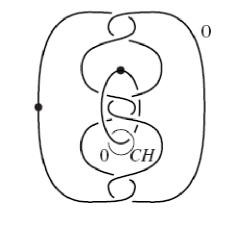
Figure 1: Link picture for the compact subset $K$

The Casson handle is given by a sequence of Whitehead links (where the unknotted component has a dot) which are linked according to the tree (see the right figure of Figure 2 for the building block and the left figure for the simplest Casson handle given by the unbranched tree).

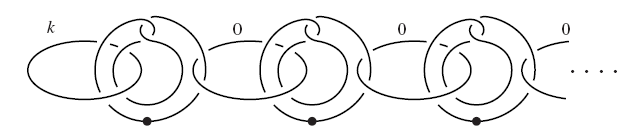
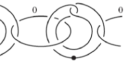
Figure 2: Building block of every Casson handle (right) and the simplest Casson handle (left).

For the construction of a 3-manifold which surrounds the compact $K$, one considers $n-$stages of the Casson handle and transforms the diagram to a real link (the dotted components are changed to usual components with framing $0$). By handle manipulations one obtains a knot so that the $n$-th (untwisted) Whitehead double of this knot represents the desired 3-manifold (by using surgery). Then our example in Figure 1 will result in the $n$-th untwisted Whitehead double of the pretzel knot $(-3,3,-3)$, Figure 3 (see [59] for the handle manipulations).

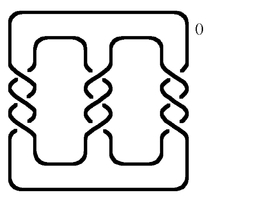
Figure 3: Pretzel knot $(-3,3,-3)$ or the knot $9_{46}$ in Rolfson notation producing the 3-manifold $Y_{1}$ by $0-$framed Dehn surgery.

Then this sequence of 3-manifolds

$$Y_{1}\to Y_{2}\to\cdots\to Y_{\infty}=Y_{r}$$

characterizes the exotic smoothness structure of $R^{4}$. The limit of this sequence $n\to\infty$ gives a wild embedded 3-manifold $Y_{r}$ whose physical relevance will be explained later.

4 Motivation: Path Integral Contribution by Exotic Smoothness

Here, we will motivate the appearance of exotic smoothness by discussing the path integral for the Einstein-Hilbert action. For simplicity, we consider general relativity without matter (using the notation of topological QFT). Space-time is a smooth oriented 4-manifold $M$ which is non-compact and without boundary. From the formal point of view (no divergences of the metric) one is able to define a boundary $\partial M$ at infinity. The classical theory is the study of the existence and uniqueness of (smooth) metric tensors $g$ on $M$ satisfying the Einstein equations subject to suitable boundary conditions. In the first order Hilbert–Palatini formulation, one specifies an $SO(1,3)$-connection $A$ together with a cotetrad field $e$ rather than a metric tensor. Fixing $A|_{\partial M}$ at the boundary, one can derive first order field equations in the interior (now called bulk) which are equivalent to the Einstein equations provided that the cotetrad is non-degenerate. The theory is invariant under space-time diffeomorphisms $M\to M$. In the particular case of the space-time $M=S^{3}\times\mathbb{R}$ (topologically), we have to consider smooth 4-manifolds $M_{i,f}$ as parts of $M$ whose boundary $\partial M_{i,f}=\Sigma_{i}\sqcup\Sigma_{f}$ is the disjoint union of two smooth 3-manifolds $\Sigma_{i}$ and $\Sigma_{f}$ to which we associate Hilbert spaces $\mathcal{H}_{j}$ of 3-geometries, $j=i,f$. These contain suitable wave functionals of connections $A|_{\Sigma_{j}}$ . We denote the connection eigenstates by $|A|_{\Sigma_{j}}\rangle$. The path integral,

$$\langle A|_{\Sigma_{f}}|T_{M}|A|_{\Sigma_{i}}\rangle=\intop_{A|\partial M_{i,f}}DA\,De\,\exp\left(\frac{i}{\hbar}S_{EH}[e,A,M_{i,f}]\right)$$ (3)

is the sum over all connections $A$ matching $A|_{\partial M_{i,f}}$, and over all $e$. It yields the matrix elements of a linear map $T_{M}:\mathcal{H}_{i}\to\mathcal{H}_{f}$ between states of 3-geometry. Our basic gravitational variables will be cotetrad $e_{a}^{I}$ and connection $A_{a}^{IJ}$ on space-time $M$ with the index $a$ to present it as 1-forms and the indices $I,J$ for an internal vector space $V$ (used for the representation of the symmetry group). Cotetrads $e$ are ‘square-roots’ of metrics and the transition from metrics to tetrads is motivated by the fact that tetrads are essential if one is to introduce spinorial matter. $e_{a}^{I}$ is an isomorphism between the tangent space $T_{p}(M)$ at any point $p$ and a fixed internal vector space $V$ equipped with a metric $\eta_{IJ}$ so that $g_{ab}=e_{a}^{I}e_{b}^{J}\eta_{IJ}$. Here we used the action

$$S_{EH}[e,A,M_{i,f},\partial M_{i,f}]=\intop_{M_{i,f}}\epsilon_{IJKL}(e^{I}\wedge e^{J}\wedge\left(dA+A\wedge A\right)^{KL})+\intop_{\partial M_{i,f}}\epsilon_{IJKL}(e^{I}\wedge e^{J}\wedge A^{KL})$$ (4)

in the notation of [3, 4]. The boundary term $\epsilon_{IJKL}(e^{I}\wedge e^{J}\wedge A^{KL})$ is equal to twice the trace over the extrinsic curvature (or the mean curvature). For fixed boundary data, (3) is a diffeomorphism invariant in the bulk. If $\Sigma_{i}=\Sigma_{f}$ are diffeomorphic, we can identify $\Sigma=\Sigma_{i}=\Sigma_{f}$ and $\mathcal{H}=\mathcal{H}_{i}=\mathcal{H}_{f}$ i.e. we close the manifold $M_{i,f}$ by identifying the two boundaries to get the closed 4-manifold $M^{\prime}$. Provided that the trace over $\mathcal{H}$ can be defined, the partition function,

$$Z(M^{\prime})=tr_{\mathcal{H}}T_{M}=\int DA\,De\,\exp\left(\frac{i}{\hbar}S_{EH}[e,A,M,\partial M]\right)$$ (5)

where the integral is now unrestricted, is a dimensionless number which depends only on the diffeomorphism class of the smooth manifold $M^{\prime}$. In case of the manifold $M_{i,f}$, the path integral (as transition amplitude) $\langle A|_{\Sigma_{f}}|T_{M}|A|_{\Sigma_{i}}\rangle$ is the diffeomorphism class of the smooth manifold relative to the boundary. The diffeomorphism class of the boundary, however, is unique and the value of the path integral depends on the topology of the boundary as well on the diffeomorphism class of the interior of $M_{i,f}$. Therefore we will shortly write

$$\langle\Sigma_{f}|T_{M}|\Sigma_{i}\rangle=\langle A|_{\Sigma_{f}}|T_{M}|A|_{\Sigma_{i}}\rangle$$

and consider the sum of manifolds like $M_{i,h}=M_{i,f}\cup_{\Sigma_{f}}M_{f,h}$ with the amplitudes

$$\langle\Sigma_{h}|T_{M}|\Sigma_{i}\rangle=\sum_{A|\Sigma_{f}}\langle\Sigma_{h}|T_{M}|\Sigma_{f}\rangle\langle\Sigma_{f}|T_{M}|\Sigma_{i}\rangle$$ (6)

where we sum (or integrate) over the connections and frames on $\Sigma_{h}$ (see [69]). Then the boundary term

$$S_{\partial}[\Sigma_{f}]=\intop_{\Sigma_{f}}\epsilon_{IJKL}(e^{I}\wedge e^{J}\wedge A^{KL})=\intop_{\Sigma_{f}}H\sqrt{h}d^{3}x$$ (7)

is needed where $H$ is the mean curvature of $\Sigma_{f}$ corresponding to the metric $h$ at $\Sigma_{f}$ (as restriction of the 4-metric). In the path integral (3), one integrates over the frames and connections. The possibility of singular frames was discussed at some places (see [103, 104]). The cotetrad field $e^{I}=e_{a}^{I}dx^{a}$ changes w.r.t. the smooth map $f:M\to M$ by $e_{a}^{I}(x)\,dx^{a}\mapsto e_{a}^{I}(x^{\prime})\,dx^{\prime a}=e_{a}^{I}(f(x))(\partial_{b}f^{a}(x))dx^{b}$. The transformation matrix $(\partial_{b}f^{a}(x))$ has maximal rank $4$ for every regular value of the smooth map, but at the critical points $x_{c}$ of $f$, some derivatives vanish and one has a smaller rank at the point $x_{c}$, called a singular point. Then there is no inverse frame (or tetrad field) at this point. Usually singular frames are of this nature and one can decompose every singular frame into a product of a regular frame and a (singular) transformation induced by a smooth map. How can one interpret these singularities? At this point one needs some differential topology. A homeomorphism can be arbitrarily and accurately approximated by smooth mappings (see [70], Theorem 2.6), i.e. in a neighborhood of a homeomorphism one always finds a smooth map. Secondly, there is a special class of smooth maps, the stable maps. Here, two smooth maps are stable equivalent if both maps agree after a diffeomorphism of the corresponding manifolds [62]. Here we are interested into smooth mappings from 4-manifolds into 4-manifolds. By a deep result of Mather [76], stable mappings for this dimension are dense in all smooth mappings of 4-manifolds. In [8], we analyzed this situation: the approximation of a homeomorphism by a stable map. If this smooth map has no singularities then we can perturb them to a diffeomorphism. For a singular map, however, we showed that it induces a change of the smoothness structure. Then, a singular frame corresponds to a regular frame in a different smoothness structure. The path integral changed the domain of integration:

$$\intop_{\mbox{regular+singular frames}}De\quad\to\intop_{\mbox{smoothness structures}}De$$

We remark that this change is unique for dimension four. No other dimension has this plethora of smoothness structures which can be used to express the singular frames.

The inclusion of exotic smoothness changed the description of trivial spaces like $\mathbb{R}^{4}$ completely. Instead of a single chart, we have now an infinite sequence of charts or an infinite sequence of 4-dimensional submanifolds. We will describe it more completely later. Each submanifold is bounded by a 3-manifold (different from a 3-sphere) and we obtain a sequence of 3-manifolds $Y_{0}\to Y_{1}\to Y_{2}\to\ldots$ characterizing the smoothness structure. The sequence of 3-manifolds divides the path integral into a product

$$\langle Y_{0}|T_{M}|Y_{1}\rangle\langle Y_{1}|T_{M}|Y_{2}\rangle\langle Y_{2}|T_{M}|Y_{3}\rangle\cdots$$

and we have to think about the boundary term (7). In [10, 20] we analyzed this term: the boundary $Y_{n}$ seen as embedding into the spacetime $M$ can be described locally as spinor $\psi$ and one obtains for the boundary term

$$\intop_{Y_{n}}H\sqrt{h}d^{3}x=\intop_{Y_{n}}\bar{\psi}D\psi\sqrt{h}d^{3}x$$ (8)

the Dirac action with the Dirac operator $D$ and $|\psi|^{2}=const.$(see [57] for the construction of $\psi$). In particular we obtained the eigenvalue equation $D\psi=H\psi$, i.e. the mean curvature is the eigenvalue of the Dirac operator which has compact spectrum (from the compactness of $Y_{n}$) or we obtained discrete levels of geometry. This result enforced us to identify the 3-manifolds (or the parts) with the matter content. Furthermore the path integral of the boundary can be carried out by an integration along $\psi$ (see [18]).With some effort [10, 20], one can extend this boundary term to a tubular neighborhood $Y_{n}\times[0,1]$ of the boundary $Y_{n}$. However, the relation (8) is only true for simple (i.e. irreducible) 3-manifolds, i.e. for complements of a knot admitting hyperbolic structure. For more complex 3-manifolds, we have the following simple scheme: the knot complements are connected by torus bundles (locally written as $T^{2}\times[0,1]$). Therefore we also have to describe these bundles by using the boundary term. In [20] we described this situation by using the geometrical properties of these bundles and we will give a short account of these ideas in subsection 9.1. Simply expressed, in this bundle one has a flow of constant curvature along the tube. The constant curvature connections are given by varying the Chern-Simons functional. Now following Floer [52], the 4-dimensional version of this flow equation is the instanton equation (or the self-dual equation) leading to the correct Yang-Mills functional (Chern-Simons gives the Pontrjagin class and the instanton equation makes it to the Yang-Mills functional). More importantly, the three possible types of torus bundles fit very good into the current scheme of three gauge field interactions (see [20] (section 8)).

5 The Action Induced by Topology

Now we have the following picture: fermions as hyperbolic knot complements and gauge bosons as torus bundles. Both components together are forming an irreducible 3-manifold which is connecting to the remaining space by a $S^{2}-$boundary (see the prime decomposition in Appendix B). This connection via $S^{2}\times[0,1]$ ($S^{2}-$bundle) is the only connection between matter and space. Here, there is only one interpretation: this $S^{2}-$bundle must be interpreted as gravity. In this section we will support this conjecture and construct the corresponding action. At first we will fix the model, i.e. let $\Sigma_{M}$ and $\Sigma_{S}$ be the 3-manifolds for matter and space, respectively. The connected sum $\#$ of both components represents the whole spatial component

$$\Sigma=\Sigma_{M}\#\Sigma_{S}=\Sigma_{M}\cup_{S^{2}}\left(S^{2}\times[0,1]\right)\cup_{S^{2}}\Sigma_{S}=\Sigma_{M}\#S^{3}\#\Sigma_{S}$$

of the spacetime. The decomposition above showed the geometry of the$S^{2}-$bundle (in the sense of Thurston, see Appendix B) to be the spherical geometry with isometry group $SO(3)$. The idea of the following construction can be simply expressed: the 2-sphere $S^{2}$ explores locally the curvature of the space where the curvature is given by the inverse volume $\frac{1}{vol(S^{2})}$ of the 2-sphere $S^{2}$. The 2-sphere can be written as a homogenous space $S^{2}=SO(3)/SO(2)$ also known as Hopf bundle. As mentioned above, the geometry of the bundle $S^{2}\times[0,1]$ (interpreted as an equator region of $S^{3}$) is the spherical geometry with isometry group $SO(3)$. So, as a local model we have an embedding of a 3-manifold (as the spatial component for a fixed time) into the spacetime with local Lorentz symmetry (represented by $SO(3,1)$). From the mathematical point of view, it is a reductive Cartan geometry[101, 102] over the homogenous space $SO(3,1)/SO(3)$, the 3-dimensional hyperbolic space. For the moment, let us extend this symmetry to the spacetime $M$ itself. A Cartan connection $A$ decomposes as a $so(3)-$valued connection $\omega$ ($so(3)$ denotes the Lie algebra of $SO(3)$) and a coframe field $e$ (with values in $so(3,1)/so(3)$) as

$$A=\omega+\frac{1}{\ell}e$$

by using the scale $\ell$(in agreement with the physical units) and with curvature

$$F = dA+A\wedge A$$

$$= (d\omega+\omega\wedge\omega)+\frac{1}{\ell^{2}}e\wedge e=R+\frac{1}{\ell^{2}}e\wedge e$$

Then for the spacetime (as 4-manifold), we interpret the Cartan connection $A$ as the connection of the frame bundle (with respect to the Lorentz structure). Now we have to think about what characterizes the $S^{2}-$bundle in a 4-manifold, i.e. a surface bundle over a surface (at least locally). It is known that a surface bundle over a surface is topologically described by the Euler class as well as the Pontrjagin class (via the Hirzebruch signature theorem). Therefore we choose the sum of the Euler and Pontrjagin class for the frame bundle as action

$$S=\intop_{M}\left(\epsilon^{ABCD}F_{AB}\wedge F_{CD}+\gamma F\wedge F\right)$$

where the Pontrjagin class is weighted by a parameter $\gamma$. Using the rules above, we obtain

$$S = \frac{1}{\ell^{2}}\intop_{M}\left(2\epsilon^{ABCD}e_{A}\wedge e_{B}\wedge R_{CD}+2\gamma e\wedge e\wedge R+\frac{(1+\gamma)}{\ell^{2}}e\wedge e\wedge e\wedge e\right)+$$

$$+\intop_{M}\left(\epsilon^{ABCD}R_{AB}\wedge R_{CD}+\gamma R\wedge R\right)\;,$$

the Einstein-Hilbert action with cosmological constant and the Holst action with Immirizo parameter as well the Euler and Pontrjagin class for the reduced bundles. In this model, the curvature is changed locally by adding a $S^{2}-$bundle. Then the scale $\ell^{2}$ has to agree with the volume of the $S^{2}$. In the action we have the coupling constant $\frac{1}{\ell^{2}}$ which has to agree with $1/L_{P}^{2}$ ($L_{P}$ Planck length) to get in contact with Einsteins theory, i.e. we must set

$$\ell=L_{P}$$

The agreement with the Einstein-Hilbert action showed that this approach can describe gravity but it does not describe the global geometry. Later we can show, however, that it must be the de Sitter space $SO(4,1)/SO(3,1)$ globally.

6 Wild Embeddings: Geometric Expression for the Quantum State

In this section we will support our main hypothesis that an exotic $\mathbb{R}^{4}$ has automatically a quantum geometry, but as noted in the introduction, we must implicitly assume that the quantum-geometrical state is realized in the exotic $\mathbb{R}^{4}$. Interestingly, it follows from the physically motivated existence of a Lorentz metric which is induced by a codimension-one foliation. Therefore we will construct the foliation and the corresponding leaf space as the space of observables (using ideas of Connes). This leaf space is a non-commutative $C^{*}-$algebra with observable algebra a factor $I\!I\!I_{1}$ von Neumann algebra. A state in this algebra can be interpreted as a wild embedding which is also motivated by the exotic smoothness structure. The classical state is the tame embedding. Then, the deformation quantization of this tame embedding is the wild embedding (see [16]). In principle, the wild embedding determines the $C^{*}-$algebra completely. This algebra is generated by holonomies along connections of constant curvature. It is known from mathematics that this algebra (forming a so-called character variety [45]) determines the geometrical structure of the 3-manifold (along the way of Thurston [84, 95]). The main structure in this approach is the fundamental group, i.e. the group of closed, non-contractible curves in a manifold. The quantization of this group (as an expression of the classical geometry) gives the so-called skein algebra of knots in this manifold. We will relate this skein algebra to the leaf space above. On the way to show this relation, we will obtain the generator of the translation from one 3-manifold into another 3-manifold, i.e. the time together with the Hamiltonian.

6.1 Exotic $\mathbb{R}^{4}$ and its Foliation

In section 4, we described the sequence of 3-manifolds

$$Y_{1}\to Y_{2}\to\cdots\to Y_{\infty}=Y_{r}$$

characterizing the exotic smoothness structure of $R^{4}$. Then $0-$framed surgery along this pretzel knot produces $Y_{1}$ whereas the $n$-th untwisted Whitehead double will give $Y_{n}$. For large $n$, the structure of the Casson handle is contained in the topology of $Y_{n}$ and in the limit $n\to\infty$ we obtain $Y_{r}$ (which is now a wild embedding $Y_{r}\subset\mathbf{R}^{4}$ in the standard $\mathbf{R}^{4}$ given by the embedding of the small exotic $R^{4}$, see above). What do we know about the structure of $Y_{n}$ or $Y_{r}$ in general? The compact subset $K$ is a 4-manifold constructed by a pair of one 1-handle and one 2-handle which topologically cancel. The boundary of $K$ is a compact 3-manifold having the first Betti number $b_{1}=1.$ This information is also contained in $Y_{r}$. By the work of Freedman [53], every Casson handle is topologically $D^{2}\times\mathbb{R}^{2}$ (relative to the attaching region) and therefore $Y_{r}$ must be the boundary of $D^{4}$ (the Casson handle trivializes $K$ to be $D^{4}$), i.e. $Y_{r}$ is a wild embedded 3-sphere $S^{3}$. Then we obtain two different descriptions of $R^{4}$:

1. as a sequence of 3-manifolds $Y_{n}$ (all having the first Betti number $b_{1}=1$) as boundaries of the neighborhood of $K$ with increasing size and

2. as a global hyperbolic space of $R^{4}\setminus K$ written as $S_{\infty}^{3}\times\mathbb{R}$ where $S_{\infty}^{3}$ is a wild embedded 3-sphere (which looks differently for different $t\in\mathbb{R}$).

The first description gives a non-trivial but smooth foliation but there is no global spatial space. In contrast to this highly non-trivial foliation, the second description gives a global foliated spacetime containing a global spatial component, the wild embedded 3-sphere. In the first description we have a complex, relational description with no global time-like slices. Here, there only is a local coordinate system (with its own eigenzeit). This relational view has the big advantage that the simplest parts are also simple submanifolds (only finite surfaces with boundary). In contrast, the second description introduces a global foliation into equal time slices. Then the complexity is contained into the spatial component which is now a wild embedding (i.e. a space with an infinite number of polygons). This second approach will be described in the next subsection. So, lets concentrate on the first approach. Every 3-manifold $Y_{n}$ admits a codimension-one ($PSL(2,\mathbb{R})-$invariant) foliation (see [17] for the details). By the description of the exotic $R^{4}$ using the sequence of 3-manifolds

$$Y_{1}\to Y_{2}\to Y_{3}\to\cdots$$

we also get a foliation of the exotic $R^{4}$. The foliation on $Y_{n}$ is defined by a $PSL(2,\mathbb{R})-$invariant one-form $\omega$ which is integrable $d\omega\wedge\omega=0$ and defines another one-form $\eta$ by $d\omega=-\eta\wedge\omega$. Then the integral

$$GV(Y_{n})=\intop_{Y_{n}}\eta\wedge d\eta$$

is known as Godbillon-Vey number $GV(Y_{n})$ with the class $gv=\eta\wedge d\eta$. From the physics point of view, it is the abelian Chern-Simons functional. The Godbillon-Vey class characterizes the codimension-one foliation for the 3-manifold $Y_{n}$ (see the Appendix B for more details). The foliation is very complicated. In [82] the local structure was analyzed. Let $\kappa,\tau$ be the curvature and torsion of a normal curve, respectively. Furthermore, let $T,N,Z$ be the frame formed by this vector field dual to the one-forms $\omega,\eta,\xi$ and let $l_{T}$ be the second fundamental form of leaf. Then the Godbillon-Vey class is locally given by

$$\eta\wedge d\eta=\kappa^{2}\left(\tau+l_{T}(N,Z)\right)\omega\wedge\eta\wedge\xi$$

where $\tau\not=0$ for $PSL(2,\mathbb{R})$ invariant foliations i.e. $[Z,N]=Z$, $[N,T]=T$ and $[Z,T]=N$. Recall that a foliation $(M,F)$ of a manifold $M$ is an integrable subbundle $F\subset TM$ of the tangent bundle $TM$. The leaves $L$ of the foliation $(M,F)$ are the maximal connected submanifolds $L\subset M$ with $T_{x}L=F_{x}\>\forall x\in L$. We denote with $M/F$ the set of leaves or the leaf space. Now one can associate to the leaf space $M/F$ a $C^{*}$-algebra $C(M,F)$ by using the smooth holonomy groupoid $G$ of the foliation (see Connes [42]). According to Connes [43], one assigns to each leaf $\ell\in X$ the canonical Hilbert space of square-integrable half-densities $L^{2}(\ell)$. This assignment, i.e. a measurable map, is called a random operator forming a von Neumann $W(M,F)$. A deep theorem of Hurder and Katok [72] for foliations with non-zero Godbillon-Vey invariant states that this foliation has to contain a factor $I\!I\!I$ von Neumann algebra. As shown in [13], the von Neumann algebra for the foliation of $Y_{n}$ and for the exotic $R^{4}$ is a factor $I\!I\!I_{1}-$algebra. For the construction of this algebra, one needs the concept of a holonomy groupoid. Foliations are determined by the holonomies of closed curves in a leaf and the transport of this closed curve together with the holonomy from the given leaf to another leaf. Now one may ask why one considers only closed curves. Let $PM$ the space of all paths in a manifold then this space admits a fibration over the space of closed paths $\Omega M$ (also called loop space) with fiber the constant paths (therefore homeomorphic to $M$), see [26]. Then, a curve is determined up to deformation (i.e. homotopy) by a closed path. Consider now a closed curve $\gamma$ in a leaf $\ell$ and let act a diffeomorphism on $\ell$. Then the curve $\gamma$ is modified as well to $\gamma^{\prime}$ but $\gamma$ and $\gamma^{\prime}$ are related by a (smooth) homotopy. Therefore to guarantee diffeomorphism invariance in this approach, one has to consider all closed curves up to homotopy. This structure can be made into a group (using concatenation of paths as group operation) called the fundamental group $\pi_{1}(\ell)$ of the leaf. Above we spoke about holonomy but a holonomy needs a connection of some bundle which we did not introduce until now. But Connes [42] described a way to circumvent this difficulty: Given a leaf $\ell$ of $(M,F)$ and two points $x,y\in\ell$ of this leaf, any simple path $\gamma$ from $x$ to $y$ on the leaf $\ell$ uniquely determines a germ $h(\gamma)$ of a diffeomorphism from a transverse neighborhood of $x$ to a transverse neighborhood of $y$. The germ of diffeomorphism $h(\gamma)$ only depends upon the homotopy class of $\gamma$ in the fundamental group of the leaf $\ell$, and is called the holonomy of the path $\gamma$. All fundamental groups of all leafs form the fundamental groupoid. The holonomy groupoid of a leaf $\ell$ is the quotient of its fundamental groupoid by the equivalence relation which identifies two paths $\gamma$ and $\gamma^{\prime}$ from $x$ to $y$ (both in $\ell$) iff $h(\gamma)=h(\gamma^{\prime})$. Then the von Neumann algebra of the foliation is the convolution algebra of the holonomy groupoid which will be constructed later for the wild embedding.

6.1.1 Intermezzo: Factor $I\!I\!I$ and Tomita-Takesaki Modular Theory

Remember a von Neumann algebra is an involutive subalgebra $M$ of the algebra of operators on a Hilbert space $H$ that has the property of being the commutant of its commutant: $(M^{\prime})^{\prime}=M$. This property is equivalent to saying that $M$ is an involutive algebra of operators that is closed under weak limits. A von Neumann algebra $M$ is said to be hyperfinite if it is generated by an increasing sequence of finite-dimensional subalgebras. Furthermore we call $M$ a factor if its center is equal to $\mathbb{C}$. It is a deep result of Murray and von Neumann that every factor $M$ can be decomposed into 3 types of factors $M=M_{I}\oplus M_{II}\oplus M_{III}$. The factor $I$ case divides into the two classes $I_{n}$ and $I_{\infty}$ with the hyperfinite factors $I_{n}=M_{n}(\mathbb{C})$ the complex square matrices and $I_{\infty}=\mathcal{L}(H)$ the algebra of all operators on an infinite-dimensional Hilbert space $H$. The hyperfinite $I\!I$ factors are given by $I\!I_{1}=Cliff_{\mathbb{C}}(E)$, the Clifford algebra of an infinite-dimensional Euclidean space $E$, and $I\!I_{\infty}=I\!I_{1}\otimes I_{\infty}$. The case $I\!I\!I$ remained mysterious for a long time. Now we know that there are three cases parametrized by a real number $\lambda\in[0,1]$: $I\!I\!I_{0}=R_{W}$ the Krieger factor induced by an ergodic flow $W$, $I\!I\!I_{\lambda}=R_{\lambda}$ the Powers factor for $\lambda\in(0,1)$ and $I\!I\!I_{1}=R_{\infty}=R_{\lambda_{1}}\otimes R_{\lambda_{2}}$ the Araki-Woods factor for all $\lambda_{1},\lambda_{2}$ with $\lambda_{1}/\lambda_{2}\notin\mathbb{Q}$. We remark that all factor $I\!I\!I$ cases are induced by infinite tensor products of the other factors. One example of such an infinite tensor space is the Fock space in quantum field theory.

The modular theory of von Neumann algebras (see also [25]) has been discovered by M. Tomita [96] in 1967 and put on solid grounds by M. Takesaki [91] around 1970. It is a very deep theory that, to every von Neumann algebra $\mathcal{M}\subset\mathcal{B}(\mathcal{H})$ acting on a Hilbert space $\mathcal{H}$, and to every vector $\xi\in\mathcal{H}$ that is cyclic, i.e. $\overline{(\mathcal{M}\xi)}=\mathcal{H}$, and separating, i.e. for $A\in\mathcal{M}$, $A\xi=0\rightarrow A=0$, associates:

• a one-parameter unitary group $t\mapsto\Delta^{it}\in\mathcal{B}(\mathcal{H})$

• and a conjugate-linear isometry $J:\mathcal{H}\to\mathcal{H}$ such that:

  $$\Delta^{it}\mathcal{M}\Delta^{-it}=\mathcal{M},\quad\forall\,t\in\mathbb{R},\qquad\text{and}\qquad J\mathcal{M}J=\mathcal{M}^{\prime},$$

  where the commutant $\mathcal{M}^{\prime}$ of $\mathcal{M}$ is defined by $\mathcal{M}^{\prime}\!:=\!\{A^{\prime}\in\mathcal{B}(\mathcal{H})\,|\,[A^{\prime},A]_{-}\!=0,\forall\,A\!\in\!\mathcal{B}(\mathcal{H})\}$.

More generally, given a von Neumann algebra $\mathcal{M}$ and a faithful normal state (more generally for a faithful normal semi-finite weight) $\omega$ on the algebra $\mathcal{M}$, the modular theory allows to create a one-parameter group of $*$-automorphisms of the algebra $\mathcal{M}$,

$$\sigma^{\omega}:t\mapsto\sigma_{t}^{\omega}\in\text{Aut}(\mathcal{M}),\qquad\text{with}\quad t\in\mathbb{R},$$

such that:

• in the Gel’fand–Naĭmark–Segal representation $\pi_{\omega}$ induced by the weight $\omega$, on the Hilbert space $\mathcal{H}_{\omega}$, the modular automorphism group $\sigma^{\omega}$ is implemented by a unitary one-parameter group $t\mapsto\Delta_{\omega}^{it}\in\mathcal{B}(\mathcal{H}_{\omega})$ i.e. we have $\pi_{\omega}(\sigma_{t}^{\omega}(x))=\Delta_{\omega}^{it}\pi_{\omega}(x)\Delta_{\omega}^{-it}$, for all $x\in\mathcal{M}$ and for all $t\in\mathbb{R}$;

• there is a conjugate-linear isometry $J_{\omega}:\mathcal{H}_{\omega}\to\mathcal{H}_{\omega}$, whose adjoint action implements a modular anti-isomorphism $\gamma_{\omega}:\pi_{\omega}(\mathcal{M})\to\pi_{\omega}(\mathcal{M})^{\prime}$, between $\pi_{\omega}(\mathcal{M})$ and its commutant $\pi_{\omega}(\mathcal{M})^{\prime}$, i.e. for all $x\in\mathcal{M}$, we have $\gamma_{\omega}(\pi_{\omega}(x))=J_{\omega}\pi_{\omega}(x)J_{\omega}$.

The operators $J_{\omega}$ and $\Delta_{\omega}$ are called respectively the modular conjugation operator and the modular operator induced by the state (weight) $\omega$. We will call “modular generator” the self-adjoint generator of the unitary one-parameter group $t\mapsto\Delta_{\omega}^{it}$ as defined by Stone’s theorem i.e. the operator

$$K_{\omega}:=\log\Delta_{\omega},\qquad\text{so that}\quad\Delta_{\omega}^{it}=e^{iK_{\omega}t}.$$ (9)

The modular automorphism group $\sigma^{\omega}$ associated to $\omega$ is the unique one-parameter automorphism group that satisfies the Kubo–Martin–Schwinger (KMS-condition) with respect to the state (or more generally a normal semi-finite faithful weight) $\omega$, at inverse temperature $\beta=-1$, i.e.

$$\omega(\sigma_{t}^{\omega}(x))=\omega(x),\qquad\forall\,x\in\mathcal{M}$$

and for all $x,y\in\mathcal{M}$.

Using Tomita-Takesaki-theory, one has a continuous decomposition (as crossed product) of any factor $I\!I\!I$ algebra $M$ into a factor $I\!I_{\infty}$ algebra $N$ together with a one-parameter group $\left(\theta_{\lambda}\right)_{\lambda\in\mathbb{R}_{+}^{*}}$ of automorphisms $\theta_{\lambda}\in Aut(N)$ of $N$, i.e. one obtains

$$M=N\rtimes_{\theta}\mathbb{R}_{+}^{*}\quad.$$ (10)

That means, there is a foliation induced from the foliation producing this $I\!I_{\infty}$ factor. Connes [43] (in section I.4 page 57ff) constructed the foliation $F^{\prime}$ canonically associated to the foliation $F$ of factor $I\!I\!I_{1}$ above having the factor $I\!I_{\infty}$ as von Neumann algebra. In our case it is the horocycle flow: Let $P$ the polygon on the hyperbolic space $\mathbb{H}^{2}$ determining the foliation above. $P$ is equipped with the hyperbolic metric $2|dz|/(1-|z|^{2})$ together with the collection $T_{1}P$ of unit tangent vectors to $P$. A horocycle in $P$ is a circle contained in $P$ which touches $\partial P$ at one point, but from the classification of factors, we know that $I\!I_{\infty}$ is also splitted into

$$I\!I_{\infty}=I\!I_{1}\otimes I_{\infty}$$

so that every factor $I\!I\!I$ is determined by the factor $I\!I_{1}$. The factor $I_{\infty}$ are the compact operators in the Hilbert space. With an important observation we will close this intermezzo. The factor $I\!I_{\infty}$ admits an action of the group $\mathbb{R}_{+}^{*}$ by automorphisms so that the crossed product (10) is the factor $I\!I\!I_{1}$. The corresponding invariant, the flow of weights $\bmod(M)$, was determined by Connes [43] to be the Godbillon-Vey invariant. Therefore the modular generator above is given by the Godbillon-Vey invariant, i.e. this invariant is the Hamiltonian of the theory.

6.1.2 Construction of a State

Then the $C^{*}$-algebra $C_{r}^{*}(M,F)$ of the foliation $(M,F)$ is the $C^{*}$-algebra $C_{r}^{*}(G)$ of the smooth holonomy groupoid $G$. For completeness we will present the explicit construction (see [43] sec. II.8). The basic elements of $C_{r}^{*}(M,F)$) are smooth half-densities with compact supports on $G$, $f\in C_{c}^{\infty}(G,\Omega^{1/2})$, where $\Omega_{\gamma}^{1/2}$ for $\gamma\in G$ is the one-dimensional complex vector space $\Omega_{x}^{1/2}\otimes\Omega_{y}^{1/2}$, where $s(\gamma)=x,t(\gamma)=y$, and $\Omega_{x}^{1/2}$ is the one-dimensional complex vector space of maps from the exterior power $\Lambda^{k}F_{x}$ ,$k=\dim F$, to $\mathbb{C}$ such that

$$\rho(\lambda\nu)=|\lambda|^{1/2}\rho(\nu)\qquad\forall\nu\in\Lambda^{k}F_{x},\lambda\in\mathbb{R}\>.$$

For $f,g\in C_{c}^{\infty}(G,\Omega^{1/2})$, the convolution product $f*g$ is given by the equality

$$(f*g)(\gamma)=\intop_{\gamma_{1}\circ\gamma_{2}=\gamma}f(\gamma_{1})g(\gamma_{2})$$

Then we define via $f^{*}(\gamma)=\overline{f(\gamma^{-1})}$ a $*$-operation making $C_{c}^{\infty}(G,\Omega^{1/2})$ into a $*$-algebra. For each leaf $L$ of $(M,F)$ one has a natural representation of $C_{c}^{\infty}(G,\Omega^{1/2})$ on the $L^{2}$ space of the holonomy covering $\tilde{L}$ of $L$. Fixing a base point $x\in L$, one identifies $\tilde{L}$ with $G_{x}=\left\{\gamma\in G,\,s(\gamma)=x\right\}$and defines the representation

$$(\pi_{x}(f)\xi)(\gamma)=\intop_{\gamma_{1}\circ\gamma_{2}=\gamma}f(\gamma_{1})\xi(\gamma_{2})\qquad\forall\xi\in L^{2}(G_{x}).$$

The completion of $C_{c}^{\infty}(G,\Omega^{1/2})$ with respect to the norm

$$||f||=\sup_{x\in M}||\pi_{x}(f)||$$

makes it into a $C^{*}$-algebra $C_{r}^{*}(M,F)$. Among all elements of the $C^{*}$-algebra, there are distinguished elements, idempotent operators or projectors having a geometric interpretation in the foliation. For later use, we will construct them explicitly (we follow [43] sec. II.8.$\!\beta$ closely). Let $N\subset M$ be a compact submanifold which is everywhere transverse to the foliation (thus $\dim(N)=\mathrm{codim}(F)$). A small tubular neighborhood $N^{\prime}$ of $N$ in $M$ defines an induced foliation $F^{\prime}$ of $N^{\prime}$ over $N$ with fibers $\mathbb{R}^{k},\,k=\dim F$. The corresponding $C^{*}$-algebra $C_{r}^{*}(N^{\prime},F^{\prime})$ is isomorphic to $C(N)\otimes\mathcal{K}$ with $\mathcal{K}$ the $C^{*}$-algebra of compact operators. In particular it contains an idempotent $e=e^{2}=e^{*}$, $e=1_{N}\otimes f\in C(N)\otimes\mathcal{K}$ , where $f$ is a minimal projection in $\mathcal{K}$. The inclusion $C_{r}^{*}(N^{\prime},F^{\prime})\subset C_{r}^{*}(M,F)$ induces an idempotent in $C_{r}^{*}(M,F)$ which is given by a closed curve in $M$ transversal to the foliation.

In case of the foliation above (of the 3-manifolds $Y_{n}$), one has the foliation of the polygon $P$ in $\mathbb{H}^{2}$ and a circle $S^{1}$ attached to every leaf of this foliation. Therefore we have the leafs $S^{1}\times[0,1]$ and the $S^{1}$is the closed curve transversal to the foliation. Then every leaf defines (using the isomorphism $\pi_{1}(S^{1}\times[0,1])=\pi_{1}(S^{1})=\mathbb{Z}$) an idempotent represented by the fiber $S^{1}$ forming a base for the GNS representation of the $C^{*}-$algebra. Now we are able to construct a state in this algebra.

A state is a linear functional $\omega:C_{r}^{*}(M,F)\to\mathbb{C}$ so that $\omega(x\cdot x^{*})\geq 0$ and $\omega(\mathbb{I}_{C_{r}^{*}(M,F)})=1$. Elements of $C_{r}^{*}(M,F)$ are half-densities with a support along some closed curve (as part of the holonomy groupoid). In a first step, one can use the GNS-representation of the $C*-$algebra $C_{r}^{*}(M,F)$ by a map $C_{r}^{*}(M,F)\to\mathcal{B}(H)$ in to the bounded operators of a Hilbert space. By the theorem of Fréchet-Riesz, every linear functional can be represented by the scalar product of the Hilbert space for some vector. To determine the linear functionals, we have to investigate the geometry of the foliation. The foliation was constructed to be $PSL(2,\mathbb{R})-$invariant, i.e. fixing the upper half space $\mathbb{H}^{2}$. Then we considered the unit tangent vectors of the tangent bundle over $\mathbb{H}^{2}$ defining the $\tilde{SL}(2,\mathbb{R})-$geometry. But more is true. Every part of the 3-manifold $Y_{n}$ is a knot/link complement with hyperbolic structure with isometry group $PSL(2,\mathbb{C})$ where the other geometric structures like $\tilde{SL}(2,\mathbb{R})$ and $PSL(2,\mathbb{R})$ embed. Here we remark the known fact that every $PSL(2,\mathbb{C})$-geometry lifts uniquely to $SL(2,\mathbb{C})$ (the double cover). Therefore, to model the holonomy, we have to choose a flat $SL(2,\mathbb{C})-$connection and write it as the well-known integral of the connection 1-form along a closed curve. The linear functional is the trace of this integral (seen as matrix using a representation of $SL(2,\mathbb{C})$) known as Wilson loop. One can use the well-known identity

$$Tr(A)\cdot Tr(B)=Tr(AB)+Tr(AB^{-1})$$

for $SL(2,\mathbb{C})$ which goes over to the Wilson loops. Let $W_{\gamma}[A]$ be the Wilson loop of a connection $A$ along the closed curve $\gamma$. Then the relation of the Wilson loops

$$W_{\gamma}[A]\cdot W_{\eta}[A]=W_{\gamma\circ\eta}[A]+W_{\gamma\circ\eta^{-1}}[A]$$

for two intersecting curves $\gamma$ and $\eta$ is known as the Mandelstam identity for intersecting loops, see Fig. 4 for a visualization.

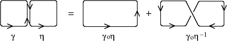
Figure 4: Mandelstam identity as skein relation (see Fig. 7 and subsection 6.3.2).

This relation is also known from another area: knot theory. There, it is the Kauffman bracket skein relation used to define the Kauffman knot polynomial. Therefore we obtain a state in the $C*-$algebra by a closed curve in the leaf which extends to a knot (an embedded, closed curve) in a submanifold of the 3-manifold defined up to the skein relation. Finally:

$$\mbox{State }\omega\mbox{ over leaf }\ell\longleftrightarrow\mbox{element of Kauffman skein module for }\mbox{$\ell\times$[0,1]}$$

We will later explain this correspondence as a deformation quantization. We will close this subsection by some remarks. Every representation $\pi_{1}(M)\to SL(2,\mathbb{C})$ defines (up to conjugacy) a flat connection. At the same time it defines also a hyperbolic structure on $Y_{n}$ (for $M=Y_{n}$). By the argumentation above, the quantized version of this geometry (as defined by the $C*-$algebra of the foliation) is given by the skein space (see subsection 6.3.2 for the definition of the skein space).

6.2 The Wild Embedded 3-Sphere = Quantum (Geometric) State

Our previous work implied that the transition from the standard $\mathbf{R}^{4}$ to a small exotic $R^{4}$ has much to do with Quantum Gravity (QG). Therefore one would expect that a submanifold in the standard $\mathbf{R}^{4}$ with an appropriated geometry represents a classical state. Before we construct this state, there is a lot to say about the wild embedded 3-sphere as a quantum state.

6.2.1 The Wild Embedded 3-Sphere

To describe this wild 3-sphere, we will construct the sequence of $Y_{n}$ by using the example of [23, 24] which was already partly explained in subsection 3.5. At first we remark that the interior of the handle body in Figure 5 is the $R^{4}$.

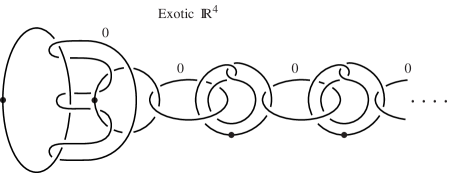
Figure 5: Handle picture of the small exotic $\mathbb{R}^{4}$, the components with the dot are 1-handles and without the dot are 2-handles.

The Casson handle for this $R^{4}$ is given by the simplest tree $\mathcal{T}_{+}$, one positive self-intersection for each level. The compact 4-manifold inside of $R^{4}$ can be seen in Figure 1 as a handle body. The 3-manifold $Y_{n}$ surrounding this compact submanifold $K$ is given by surgery ($0-$framed) along the link in Figure 5 with a Casson handle of $n-$levels. In [59], this case is explicitly discussed. $Y_{n}$ is given by $0-$framed surgery along the $n$-th untwisted Whitehead double of the pretzel $(-3,3-3)$ knot (see Figure 3). Obviously, there is a sequence of inclusions

$$\ldots\subset Y_{n-1}\subset Y_{n}\subset Y_{n+1}\subset\ldots\to Y_{\mathcal{T}_{+}}$$

with the 3-manifold $Y_{\mathcal{T}_{+}}$ as limit. Let $\mathcal{K}_{+}$ be the corresponding (wild) knot, i.e. the $\infty$-th untwisted Whitehead double of the pretzel knot $(-3,3,-3)$ (or the knot $9_{46}$ in Rolfson notation). The surgery description of $Y_{\mathcal{T}_{+}}$induces the decomposition

$$Y_{\mathcal{T}_{+}}=C(\mathcal{K}_{+})\cup\left(D^{2}\times S^{1}\right)\qquad C(\mathcal{K}_{+})=S^{3}\setminus\left(\mathcal{K}_{+}\times D^{2}\right)$$ (11)

where $C(\mathcal{K}_{+})$ is the knot complement of $\mathcal{K}_{+}$. In [33], the splitting of knot complements was described. Let $K_{9_{46}}$ be the pretzel knot $(-3,3,-3)$ and let $L_{Wh}$ be the Whitehead link (with two components). Then the complement $C(K_{9_{46}})$ has one torus boundary whereas the complement $C(L_{Wh})$ has two torus boundaries. Now according to [33], one obtains the splitting

$$C(\mathcal{K}_{+})=C(L_{Wh})\cup_{T^{2}}\cdots\cup_{T^{2}}C(L_{Wh})\cup_{T^{2}}C(K_{9_{46}})$$

and we will describe each part separately (see Figure 6).

Figure 6: Schematic picture for the splitting of the knot complement $C(\mathcal{K}_{+})$ (above) and in the more general case $C(\mathcal{K_{T}})$ (below).

At first the knot $K_{9_{46}}$ is a hyperbolic knot, i.e. the interior of the 3-manifold $C(K_{9_{46}})$ admits a hyperbolic metric. By the work of Gabai [60], $C(K_{9_{46}})$admits a codimension-one foliation. The Whitehead link is a hyperbolic link but we need more: the Whitehead link is a fibered link of genus $1$. That is, there is a fibration of the link complement $\pi:C(L_{Wh})\to S^{1}$ over the circle so that $\pi^{-1}(p)$ is a surface of genus $1$ (Seifert surface) for all $p\in S^{1}$. Now we will also describe the changes for a general tree. At first we will modify the Whitehead link: we duplicate the linked circle, i.e. there are as many circles as branching in the tree to get the link $Wh_{n}$ with $n+1$ components. Then the complement of $Wh_{n}$ has also $n+1$ torus boundaries and it also fibers over $S^{1}$. With the help of $Wh_{n}$ we can build every tree $\mathcal{T}$. Now the 3-manifold $Y_{\mathcal{T}}$ is given by $0-$framed surgery along the $\infty$-th untwisted ramified (usage of $Wh_{n}$) Whitehead double of a knot $k$, denoted by the link $\mathcal{K_{T}}$. The tree $\mathcal{T}$ has one root, then $Y_{\mathcal{T}}$ is given by

$$Y_{\mathcal{T}}=C(\mathcal{K_{T}})\cup\left(D^{2}\times S^{1}\right)$$

and the complement $C(\mathcal{K_{T}})$ splits like the tree into complements of $Wh_{n}$ and one copy of $C(k)$ (see Figure 6). Using a deep result of Freedman [53], we obtain:
$Y_{\mathcal{T}}$ is a wild embedded 3-sphere $S_{\infty}^{3}$.

6.2.2 Reconstruction of the Spatial Space by Using a State

Our result about the existence of a codimension-one foliation for $Y_{\mathcal{T}}$ can be simply expressed: foliations are characterized by the holonomy properties of the leafs. This principle is also the corner stone for the usage of non-commutative geometry as description of the leaf space. In the previous subsection, we already characterized the state as an element of the Kauffman skein module. Here we are interested in a reconstruction of the underlying space but now assuming a global foliation so that we will obtain the whole spatial space.

Starting point is the state constructed in the subsection 6.1.2. Here, we got a relation between the state $\omega$ as linear functional over the algebra and the Kauffman skein module. Using this relation, we consider a leaf $\ell=S^{1}\times[0,1]$ and the 3-dimensional extension as solid torus $S^{1}\times D^{2}$. The Kauffman skein module $K(S^{1}\times D^{2})$ is polynomial algebra with one generator (the loop around $S^{1}$). Now we consider one 3-manifold $Y_{n}$ with the corresponding foliation. Using the splitting above, the Kauffman skein module $K(Y_{n})$ is determined by the skein module for the parts, i.e. by the knot complements. Therefore we have to consider the skein module for hyperbolic 3-manifolds. Hyperbolic 3-manifolds contain special surfaces, called essential or incompressible surfaces, see Appendix C. It is known [36] that the skein module of 3-manifolds containing essential surfaces is not finitely generated. Therefore, the state itself is not finitely generated. If we use the leaf $S^{1}\times D^{2}$ as a local model for one generator then we will obtain an infinitely complicated 3-manifold made from pieces $S^{1}\times D^{2}$ so that the corresponding generators are not related to each other. An example of this structure is the Whitehead manifold having a non-finitely generated Kauffman skein module [1]. In general we will obtain a wild embedded 3-manifold by using this simple pieces. By the argumentation in the previous subsection we know that this wild embedded 3-manifold is the wild embedded 3-sphere $Y_{\mathcal{T}}$. Finally we obtain:

$$\mbox{State }\omega\longleftrightarrow\mbox{\mbox{wild embedded 3-sphere }}Y_{\mathcal{T}}$$

the state $\omega$ is realized by some wild embedded 3-sphere.

6.2.3 Construction of the Operator Algebra

Following [16] we will construct a $C^{*}-$algebra from the wild embedded 3-sphere. Let $I:S^{3}\to\mathbb{R}^{4}$ be a wild embedding of codimension-one so that $I(S^{3})=S_{\infty}^{3}=Y_{\mathcal{T}}$. Now we consider the complement $\mathbb{R}^{4}\setminus I(S^{3})$ which is non-trivial, i.e. $\pi_{1}(\mathbb{R}^{4}\setminus I(S^{3}))=\pi\not=1$. Now we define the $C^{*}-$algebra $C^{*}(\mathcal{G},\pi$) associated to the complement $\mathcal{G}=\mathbb{R}^{4}\setminus I(S^{3})$ with group $\pi=\pi_{1}(\mathcal{G})$. If $\pi$ is non-trivial then this group is not finitely generated. From an abstract point of view, we have a decomposition of $\mathcal{G}$ by an infinite union

$$\mathcal{G}=\bigcup_{i=0}^{\infty}C_{i}$$

of ’level sets’ $C_{i}$. Then every element $\gamma\in\pi$ lies (up to homotopy) in a finite union of levels.

The basic elements of the $C^{*}-$algebra $C^{*}(\mathcal{G},\pi$) are smooth half-densities with compact supports on $\mathcal{G}$, $f\in C_{c}^{\infty}(\mathcal{G},\Omega^{1/2})$, where $\Omega_{\gamma}^{1/2}$ for $\gamma\in\pi$ is the one-dimensional complex vector space of maps from the exterior power $\Lambda^{k}L$ ($\dim L=k$), of the union of levels $L$ representing $\gamma$, to $\mathbb{C}$ such that

$$\rho(\lambda\nu)=|\lambda|^{1/2}\rho(\nu)\qquad\forall\nu\in\Lambda^{2}L,\lambda\in\mathbb{R}\>.$$

For $f,g\in C_{c}^{\infty}(\mathcal{G},\Omega^{1/2})$, the convolution product $f*g$ is given by the equality

$$(f*g)(\gamma)=\intop_{\gamma_{1}\circ\gamma_{2}=\gamma}f(\gamma_{1})g(\gamma_{2})$$

with the group operation $\gamma_{1}\circ\gamma_{2}$ in $\pi$. Then we define via $f^{*}(\gamma)=\overline{f(\gamma^{-1})}$ a $*$operation making $C_{c}^{\infty}(\mathcal{G},\Omega^{1/2})$ into a $*$algebra. Each level set $C_{i}$ consists of simple pieces (in case of Alexanders horned sphere, we will explain it below) denoted by $T$. For these pieces, one has a natural representation of $C_{c}^{\infty}(\mathcal{G},\Omega^{1/2})$ on the $L^{2}$ space over $T$. Then one defines the representation

$$(\pi_{x}(f)\xi)(\gamma)=\intop_{\gamma_{1}\circ\gamma_{2}=\gamma}f(\gamma_{1})\xi(\gamma_{2})\qquad\forall\xi\in L^{2}(T),\forall x\in\gamma.$$

The completion of $C_{c}^{\infty}(\mathcal{G},\Omega^{1/2})$ with respect to the norm

$$||f||=\sup_{x\in\mathcal{G}}||\pi_{x}(f)||$$

makes it into a $C^{*}$-algebra $C_{c}^{\infty}(\mathcal{G},\pi$). Finally we are able to define the $C^{*}-$algebra associated to the wild embedding. Using a result in [16], one can show that the corresponding von Neumann algebra is the factor $I\!I\!I_{1}$.

Among all elements of the $C^{*}$-algebra, there are distinguished elements, idempotent operators or projectors having a geometric interpretation. For later use, we will construct them explicitly (we follow [43] sec. $II.8.\beta$ closely). Let $Y_{\mathcal{T}}\subset\mathbb{R}^{4}$ be the wild submanifold. A small tubular neighborhood $N^{\prime}$ of $Y_{\mathcal{T}}$ in $\mathbb{R}^{4}$ defines the corresponding $C^{*}$-algebra $C_{c}^{\infty}(N^{\prime},\pi_{1}(\mathbb{R}^{4}\setminus N^{\prime}))$ is isomorphic to $C_{c}^{\infty}(\mathcal{G},\pi_{1}(\mathbb{R}^{4}\setminus I(S^{3}))\otimes\mathcal{K}$ with $\mathcal{K}$ the $C^{*}$-algebra of compact operators. In particular it contains an idempotent $e=e^{2}=e^{*}$, $e=1_{N}\otimes f\in C_{c}^{\infty}(\mathcal{G},\pi_{1}(\mathbb{R}^{4}\setminus I(S^{3})))\otimes\mathcal{K}$ , where $f$ is a minimal projection in $\mathcal{K}$. It induces an idempotent in $C_{c}^{\infty}(\mathcal{G},\pi_{1}(\mathbb{R}^{4}\setminus I(S^{3})))$. By definition, this idempotent is given by a closed curve in the complement $\mathbb{R}^{4}\setminus I(S^{3})$. These projection operators form the basis in this algebra

6.3 Reconstructing the Classical State

In this section we will describe a way from a (classical) Poisson algebra to a quantum algebra by using deformation quantization. Therefore we will obtain a positive answer to the question: Does the $C^{*}-$algebra of the foliation (as well of a wild (specific) embedding) comes from a (deformation) quantization? Of course, this question cannot be answered in all generality, but for our example we will show that the enveloping von Neumann algebra of foliation and of this wild embedding is the result of a deformation quantization using the classical Poisson algebra (of closed curves) of the tame embedding. This result shows two things: the wild embedding can be seen as a quantum state and the classical state is a tame embedding.

6.3.1 Intermezzo 1: The Observable Algebra and its Poisson Structure

In this section we will describe the formal structure of a classical theory coming from the algebra of observables using the concept of a Poisson algebra. In quantum theory, an observable is represented by an hermitean operator having the spectral decomposition via projectors or idempotent operators. The coefficient of the projector is the eigenvalue of the observable or one possible result of a measurement. At least one of these projectors represents (via the GNS representation) a quasi-classical state. Thus, to construct the substitute of a classical observable algebra with Poisson algebra structure, we have to concentrate on the idempotents in the $C^{*}$-algebra. Now we will see that the set of closed curves on a surface has the structure of a Poisson algebra. Let us start with the definition of a Poisson algebra.

Let $P$ be a commutative algebra with unit over $\mathbb{R}$ or $\mathbb{C}$. A Poisson bracket on $P$ is a bilinearform $\left\{\>,\>\right\}:P\otimes P\to P$ fulfilling the following 3 conditions:

1. anti-symmetry $\left\{a,b\right\}=-\left\{b,a\right\}$

2. Jacobi identity $\left\{a,\left\{b,c\right\}\right\}+\left\{c,\left\{a,b\right\}\right\}+\left\{b,\left\{c,a\right\}\right\}=0$

3. derivation $\left\{ab,c\right\}=a\left\{b,c\right\}+b\left\{a,c\right\}$.

Then a Poisson algebra is the algebra $(P,\{\,,\,\})$.

Now we consider a surface $S$ together with a closed curve $\gamma$. Additionally we have a Lie group $G$ given by the isometry group. The closed curve is one element of the fundamental group $\pi_{1}(S)$. From the theory of surfaces we know that $\pi_{1}(S)$ is a free abelian group. Denote by $Z$ the free $\mathbb{K}$-module ($\mathbb{K}$ a ring with unit) with the basis $\pi_{1}(S)$, i.e. $Z$ is a freely generated $\mathbb{K}$-module. Recall Goldman’s definition of the Lie bracket in $Z$ (see [61]). For a loop $\gamma:S^{1}\to S$ we denote its class in $\pi_{1}(S)$ by $\left\langle\gamma\right\rangle$. Let $\alpha,\beta$ be two loops on $S$ lying in general position. Denote the (finite) set $\alpha(S^{1})\cap\beta(S^{1})$ by $\alpha\#\beta$. For $q\in\alpha\#\beta$ denote by $\epsilon(q;\alpha,\beta)=\pm 1$ the intersection index of $\alpha$ and $\beta$ in $q$. Denote by $\alpha_{q}\beta_{q}$ the product of the loops $\alpha,\beta$ based in $q$. Up to homotopy the loop $(\alpha_{q}\beta_{q})(S^{1})$ is obtained from $\alpha(S^{1})\cup\beta(S^{1})$ by the orientation preserving smoothing of the crossing in the point $q$. Set

$$[\left\langle\alpha\right\rangle,\left\langle\beta\right\rangle]=\sum_{q\in\alpha\#\beta}\epsilon(q;\alpha,\beta)(\alpha_{q}\beta_{q})\quad.$$ (12)

According to Goldman [61] (theorem 5.2), the bilinear pairing $[\,,\,]:Z\times Z\to Z$ given by (12) on the generators is well defined and makes $Z$ a Lie algebra. The algebra $Sym(Z)$ of symmetric tensors is then a Poisson algebra (see Turaev [98]).

The whole approach seems natural for the construction of the Lie algebra $Z$ but the introduction of the Poisson structure is an artificial act. From the physical point of view, the Poisson structure is not the essential part of classical mechanics. More important is the algebra of observables, i.e. functions over the configuration space forming the Poisson algebra. For the foliation discussed above, we already identified the observable algebra (the holonomy along closed curves) as well the corresponding group to be $SL(2,\mathbb{C})$. Therefore for the following, we will set $G=SL(2,\mathbb{C})$.

Now we introduce a principal $G$ bundle on $S$, representing a geometry on the surface. This bundle is induced from a $G$ bundle over $S\times[0,1]$ having always a flat connection. Alternatively one can consider a homomorphism $\pi_{1}(S)\to G$ represented as holonomy functional

$$hol(\omega,\gamma)=\mathcal{P}\exp\left(\int\limits_{\gamma}\omega\right)\in G$$ (13)

with the path ordering operator $\mathcal{P}$ and $\omega$ as flat connection (i.e. inducing a flat curvature $\Omega=d\omega+\omega\wedge\omega=0$). This functional is unique up to conjugation induced by a gauge transformation of the connection. Thus we have to consider the conjugation classes of maps

$$hol:\pi_{1}(S)\to G$$

forming the space $X(S,G)$ of gauge-invariant flat connections of principal $G$ bundles over $S$. Now (see [85]) we can start with the construction of the Poisson structure on $X(S,G)$, based on the Cartan form as the unique bilinearform of a Lie algebra. As discussed above we will use the Lie group $G=SL(2,\mathbb{C})$ but the whole procedure works for every other group too. Now we consider the standard basis

$$X=\left(\begin{array}[]{cc}0&1\\ 0&0\end{array}\right)\quad,\qquad H=\left(\begin{array}[]{cc}1&0\\ 0&-1\end{array}\right)\quad,\qquad Y=\left(\begin{array}[]{cc}0&0\\ 1&0\end{array}\right)$$ (14)

of the Lie algebra $sl(2,\mathbb{C})$ with $[X,Y]=H,\,[H,X]=2X,\,[H,Y]=-2Y$. Furthermore there is the bilinearform $B:sl_{2}\otimes sl_{2}\to\mathbb{C}$ written in the standard basis as

$$\left(\begin{array}[]{ccc}0&0&-1\\ 0&-2&0\\ -1&0&0\end{array}\right)$$

Now we consider the holomorphic function $f:SL(2,\mathbb{C})\to\mathbb{C}$ and define the gradient $\delta_{f}(A)$ along $f$ at the point $A$ as $\delta_{f}(A)=Z$ with $B(Z,W)=df_{A}(W)$ and

$$df_{A}(W)=\left.\frac{d}{dt}f(A\cdot\exp(tW))\right|_{t=0}\quad.$$

The calculation of the gradient $\delta_{tr}$ for the trace $tr$ along a matrix

$$A=\left(\begin{array}[]{cc}a_{11}&a_{12}\\ a_{21}&a_{22}\end{array}\right)$$

is given by

$$\delta_{tr}(A)=-a_{21}Y-a_{12}X-\frac{1}{2}(a_{11}-a_{22})H\quad.$$

Given a representation $\rho\in X(S,SL(2,\mathbb{C}))$ of the fundamental group and an invariant function $f:SL(2,\mathbb{C})\to\mathbb{R}$ extendable to $X(S,SL(2,\mathbb{C}))$. Then we consider two conjugacy classes $\gamma,\eta\in\pi_{1}(S)$ represented by two transversal intersecting loops $P,Q$ and define the function $f_{\gamma}:X(S,SL(2,\mathbb{C})\to\mathbb{C}$ by $f_{\gamma}(\rho)=f(\rho(\gamma))$. Let $x\in P\cap Q$ be the intersection point of the loops $P,Q$ and $c_{x}$ a path between the point $x$ and the fixed base point in $\pi_{1}(S)$. Then we define $\gamma_{x}=c_{x}\gamma c_{x}^{-1}$ and $\eta_{x}=c_{x}\eta c_{x}^{-1}$. Finally we get the Poisson bracket

$$\left\{f_{\gamma},f^{\prime}_{\eta}\right\}=\sum_{x\in P\cap Q}sign(x)\>B(\delta_{f}(\rho(\gamma_{x})),\delta_{f^{\prime}}(\rho(\eta_{x})))\quad,$$

where $sign(x)$ is the sign of the intersection point $x$. Thus,

The space $X(S,SL(2,\mathbb{C}))$ has a natural Poisson structure (induced by the bilinear form (12) on the group) and the Poisson algebra $(X(S,SL(2,\mathbb{C}),\left\{\,,\,\right\})$ of complex functions over them is the algebra of observables.

6.3.2 Intermezzo 2: Drinfeld-Turaev Quantization

Now we introduce the ring $\mathbb{C}[[h]]$ of formal polynomials in $h$ with values in $\mathbb{C}$. This ring has a topological structure, i.e. for a given power series $a\in\mathbb{C}[[h]]$ the set $a+h^{n}\mathbb{C}[[h]]$ forms a neighborhood. Now we define

A Quantization of a Poisson algebra $P$ is a $\mathbb{C}[[h]]$ algebra $P_{h}$ together with the $\mathbb{C}$-algebra isomorphism $\Theta:P_{h}/hP\to P$ so that

1. the module $P_{h}$ is isomorphic to $V[[h]]$ for a $\mathbb{C}$ vector space $V$

2. let $a,b\in P$ and $a^{\prime},b^{\prime}\in P_{h}$ be $\Theta(a)=a^{\prime}$, $\Theta(b)=b^{\prime}$ then

$$\Theta\left(\frac{a^{\prime}b^{\prime}-b^{\prime}a^{\prime}}{h}\right)=\left\{a,b\right\}\;.$$

One speaks of a deformation of the Poisson algebra by using a deformation parameter $h$ to get a relation between the Poisson bracket and the commutator. Therefore we have the problem to find the deformation of the Poisson algebra $(X(S,SL(2,\mathbb{C})),\left\{\,,\,\right\})$. The solution to this problem can be found via two steps:

1. at first find another description of the Poisson algebra by a structure with one parameter at a special value and

2. secondly vary this parameter to get the deformation.

Fortunately both problems were already solved (see [97, 98]). The solution of the first problem is expressed in the theorem:

The skein module $K_{-1}(S\times[0,1])$ (i.e. $t=-1$) has the structure of an algebra isomorphic to the Poisson algebra $(X(S,SL(2,\mathbb{C})),\left\{\,,\,\right\})$. (see also [34, 38])

Then we have also the solution of the second problem:

The skein algebra $K_{t}(S\times[0,1])$ is the quantization of the Poisson algebra $(X(S,SL(2,\mathbb{C})),\left\{\,,\,\right\})$ with the deformation parameter $t=\exp(h/4)$.(see also [38])

To understand these solutions we have to introduce the skein module $K_{t}(M)$ of a 3-manifold $M$ (see [81]). For that purpose we consider the set of links $\mathcal{L}(M)$ in $M$ up to isotopy and construct the vector space $\mathbb{C}\mathcal{L}(M)$ with basis $\mathcal{L}(M)$. Then one can define $\mathbb{C}\mathcal{L}[[t]]$ as ring of formal polynomials having coefficients in $\mathbb{C}\mathcal{L}(M)$. Now we consider the link diagram of a link, i.e. the projection of the link to the $\mathbb{R}^{2}$ having the crossings in mind. Choosing a disk in $\mathbb{R}^{2}$ so that one crossing is inside this disk. If the three links differ by the three crossings $L_{oo},L_{o},L_{\infty}$ (see figure 7) inside of the disk then these links are skein-related.

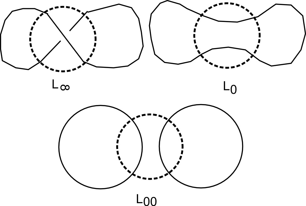
Figure 7: Crossings $L_{\infty},L_{o},L_{oo}$.

Then in $\mathbb{C}\mathcal{L}[[t]]$ one writes the skein relation $L_{\infty}-tL_{o}-t^{-1}L_{oo}$. Furthermore let $L\sqcup O$ be the disjoint union of the link with a circle and one writes the framing relation $L\sqcup O+(t^{2}+t^{-2})L$. Let $S(M)$ be the smallest submodule of $\mathbb{C}\mathcal{L}[[t]]$ containing both relations. Then we define the Kauffman bracket skein module by $K_{t}(M)=\mathbb{C}\mathcal{L}[[t]]/S(M)$. We list the following general results about this module:

• The module $K_{-1}(M)$ for $t=-1$ is a commutative algebra.

• Let $S$ be a surface, then $K_{t}(S\times[0,1])$ carries the structure of an algebra.

The algebraic structure of $K_{t}(S\times[0,1])$ can be simply seen by using the diffeomorphism between the sum $S\times[0,1]\cup_{S}S\times[0,1]$ along $S$ and $S\times[0,1]$. Then the product $ab$ of two elements $a,b\in K_{t}(S\times[0,1])$ is a link in $S\times[0,1]\cup_{S}S\times[0,1]$ corresponding to a link in $S\times[0,1]$ via the diffeomorphism. The algebra $K_{t}(S\times[0,1])$ is in general non-commutative for $t\not=-1$. For the following we will omit the interval $[0,1]$ and denote the skein algebra by $K_{t}(S)$.

In subsection 6.1.2, we described the state as an element of the Kauffman skein module $K_{t}(\ell)$ of the leaf $\ell$. Now we obtained also that the observable algebra is the Kauffman skein module again. How does this whole story fit into the description of the observable algebra for the foliation as factor $I\!I\!I_{1}$? In [58], it was shown that the Kauffman bracket skein module of a cylinder over the torus embeds as a subalgebra of the noncommutative torus. However, the noncommutative torus can be seen as the leaf space of the Kronecker foliation of the torus leading to the factor $I\!I_{\infty}$. Then by using (10), we obtain the factor $I\!I\!I_{1}$ back. We will use this relation in the next section to get the quantum action.

7 Action at the Quantum Level

Above, we used the foliation to get quantum states which agreed with the deformation quantization of a classical state. Central point in our argumentation is the construction of the $C^{*}-$algebra with the corresponding von Neumann algebra as observable algebra. This von Neumann algebra is a factor $I\!I\!I_{1}$. By using the Tomita-Takesaki modular theory, there is a relation to the factor $I\!I_{\infty}$ by using an action of the group $\mathbb{R}_{+}^{*}$ by automorphisms of a Lebesgue measure space leading to the decomposition of the factor $I\!I\!I_{1}$. This action is related to an invariant, the flow of weights mod(M). The main property of the factor $I\!I\!I_{1}$ is the constant flow of weights mod(M). Connes [42, 43] described the flow of weights as a bundle of densities over the leaf space, i.e. the $\mathbb{R}_{+}^{*}$ homogeneous space of nonzero maps. In case of foliation considered above, this density is constant and we can naturally identify this density with the volume of the submanifold defining the foliation. By definition, this volume is given by the Godbillon-Vey invariant (see eqn. (34) in Appendix B, the circle in the fiber has unit size). This invariant can be seen as an element of $H^{3}(BG,\mathbb{R})$ with the holonomy groupoid $G$ of the foliation. As shown by Connes [42, 43], the Godbillon-Vey class $GV$ can be expressed as a cyclic cohomology class (the so-called flow of weights)

$$GV_{HC}\in HC^{2}(C_{c}^{\infty}(G))$$

of the $C^{*}-$algebra for the foliation. Then we define an expression

$$S=Tr_{\omega}\left(GV_{HC}\right)$$

uniquely associated to the foliation ($Tr_{\omega}$ is the Dixmier trace). The expression $S$ generates the action on the factor by

$$\Delta_{\omega}^{it}=exp(i\,S)$$

so that $S$ is the action or the Hamiltonian multiplied by the time (see (9)). It is an operator which defines the dynamics by acting on the states. For explicit calculations we have to evaluate this operator. One way is the usage of the relation between the foliation and the wild embedding. This wild embedding is determined by the fundamental group $\pi$ of its complement. In [16], we discussed the properties of this group $\pi$. It is a perfect group, i.e. every element is generated by a commutator. Then a representation of this group into some other group like $GL(\mathbb{C})$ (the limit of $GL(n,\mathbb{C})$ for $n\to\infty$) reduces to the representation of the maximal perfect subgroup. For that purpose we consider the representation of the group $\pi$ into the group $E(\mathbb{C})$ of elementary matrices, which is the perfect subgroup of $GL(\mathbb{C})$. Then we obtain matrix-valued functions $X^{\mu}\in C_{c}^{\infty}(E(\mathbb{C}))$ as the image of the generators of $\pi$ w.r.t. the representation $\pi\to E(\mathbb{C})$ labeled by the dimension $\mu=1,\ldots,4$ of the embedding space $R^{n}$. Via the representation $\iota:\pi\to E(\mathbb{C})$, we obtain a cyclic cocycle in $HC^{2}(C_{c}^{\infty}(E(\mathbb{C}))$ generated by a suitable Fredholm operator $F$. Here we use the standard choice $F=D|D|^{-1}$ with the Dirac operator $D$ acting on the functions in $C_{c}^{\infty}(E(\mathbb{C}))$. Then the cocycle in $HC^{2}(C_{c}^{\infty}(E(\mathbb{C}))$ can be expressed by

$$\iota_{*}GV_{HC}=\eta_{\mu\nu}[F,X^{\mu}][F,X^{\nu}]$$

using a metric $\eta_{\mu\nu}$in $R^{4}$ via the pull-back using the representation $\iota:\pi\to E(\mathbb{C})$. Finally we obtain the action

$$S=Tr_{\omega}([F,X^{\mu}][F,X_{\mu}])=Tr_{\omega}([D,X^{\mu}][D,X_{\mu}]|D|^{-2})$$ (15)

which can be evaluated by using the heat-kernel of the Dirac operator $D$. The appearance of the heat kernel is a sign for a relation to quantum field theory where the heat kernel is a very convenient tool for studying one-loop divergences, anomalies and various asymptotics of the effective action.

Away from this operator expression for the Godbillon-Vey invariant, there are geometrical evaluations which are not defined on the leaf space but rather on the whole manifold. As mentioned above, this invariant admits values in the real numbers and we can evaluate them according to the type of the number: for integer values one obtains the Euler class and for rational numbers the Pontrjagin class (for the corresponding bundles). Therefore using the ideas of section 5, we obtain the Einstein-Hilbert and the Holst action but also a correction given by irrational values of the Godbillon-Vey number.

8 The Scaling Behavior of the Action

A good test for the theory is the dependence of the action (15) on the scale. The theory has a strong geometrical flavor and therefore the scaling behavior can be understood by a geometrical construction using the exotic $R^{4}$. As explained above, the central point in the construction is the Casson handle. From the scaling point of view, the Casson handle contains disks of any size (with respect to the embedding $R^{4}\hookrightarrow\mathbf{R^{4}}$). The long scales are given by the first levels of the Casson handle whereas the small scales are represented by the higher levels of the Casson handle.

8.1 Long-scale Behavior (Einstein-Hilbert Action)

Let us consider the small exotic $R^{4}$. From the physics point of view, the large scale is given by the first levels of the Casson handle. In the construction of the foliation of $R^{4}$, the first levels describe a polygon in the hyperbolic space $\mathbb{H}^{2}$ with a finite and small number of vertices. The Godbillon-Vey number of this foliation is given by the volume of this polygon. In principle, it is also true for the inclusion of the higher levels (and also for the whole Casson handle) but every higher level gives only a very small contribution to the Godbillon-Vey number. Therefore, the first levels of the Casson handle can be simply characterized by the Godbillon-Vey number, i.e. by the size of the polygon in the scale $r$. Then the Godbillon-Vey number is given by $GV=r^{2}$. In [16] we analyzed this situation and found the relation

$$GV\stackrel{{\scriptstyle r\to\infty}}{{=}}r^{2}\intop_{D^{2}}\left(g_{\mu\nu}\partial_{k}\xi^{\mu}\partial^{k}\xi^{\nu}\right)d^{2}x$$

to the Godbillon-Vey number. Here we integrate over the disk (equal to the polygon) which is used to define the foliation. This model is the non-linear sigma model (for the embedding of the disk into $Y_{n}$ with metric $g$) depending on the scale $r^{2}$. The scaling behavior of this model was studied in [56] and one obtains the RG flow equation

$$\frac{\partial}{\partial r^{2}}g_{\mu\nu}=R_{\mu\nu}+\frac{1}{r^{2}}\left(R_{\mu\lambda\kappa\iota}R_{\nu}^{\lambda\kappa\iota}\right)+O(r^{-4})$$ (16)

reducing to the Ricci flow equations for large scales ($r\to\infty$). The fixed point of this flow are geometries of constant curvature (used to prove the Thurston geometrization conjecture). Therefore in the classical limit of large scales, we obtain a geometry of the 3-manifold of constant curvature whereas for small scales one has to take into account higher curvature corrections. On the spacetime, one has also flow equations from one 3-manifold of constant curvature to another 3-manifold of constant curvature. This flow equation is equivalent to the (anti-)self-dual curvature (or instantons) by using the gradient flow of the Chern-Simons functional [52]. This approach has much in common with the non-linear graviton of Penrose [79]. We will explain these ideas in subsection 9.1.

8.2 Short-scale Behavior

For the short scale, we need the full power of the Casson handle. As a first step we can evaluate the action (15) so that the Dirac operator $D$ acts on usual square-integrable functions, so that $[D,X^{\mu}]=dX^{\mu}$ is finite. Then the action (15) reduces to

$$S=Tr_{\omega}(\eta_{\mu\nu}(\partial_{k}X^{\mu}\partial^{k}X^{\nu})|D|^{-2})$$

where $\mu,\nu=1,\ldots,4$ is the index for the coordinates on $R^{4}$ and $k=1,2$ represents the index of the disk (inside of the Casson handle). Now we will choose a small fluctuation $\xi^{k}$ of a fixed embedding of the disk in the Casson handle given by $X^{\mu}=(x^{k}+\xi^{\mu})\delta_{k}^{\mu}$ with $\partial_{l}x^{k}=\delta_{l}^{k}$. Then we obtain

$$\partial_{k}X^{\mu}\partial^{k}X^{\nu}=\delta_{k}^{\mu}\delta_{k}^{\nu}(1+\partial_{k}\xi^{\mu})(1+\partial_{k}\xi^{\nu})$$

and we use a standard argument to neglect the terms linear in $\partial\xi$: fluctuations have no preferred direction and therefore only the square contributes. Then we have

$$S=Tr_{\omega}(\eta_{\mu\nu}(\delta_{k}^{\mu}\delta_{k}^{\nu}+\partial_{k}\xi^{\mu}\partial^{k}\xi^{\nu})|D|^{-2})$$

for the action. By using a result of [43] one obtains for the Dixmier trace

$$Tr_{\omega}(|D|^{-2})=2\intop_{D^{2}}*(\Phi_{1})$$

with the first coefficient $\Phi_{1}$ of the heat kernel expansion [21]

$$\Phi_{1}=\frac{1}{6}R$$

and the action simplifies to

$$S=\intop_{D^{2}}\left(\frac{2}{3}R+\partial_{k}\xi^{\mu}\partial^{k}\xi^{\nu}\frac{1}{3}R\right)dvol(D^{2})$$ (17)

for the main contributions where $R$ is the scalar curvature of the embedded disk $D^{2}$. Again, but now for small fluctuations, we obtain the flow equation (16) but we have to consider the small case $r\to 0$. Then we have to take arbitrary curvature contributions into account. This short calculation showed that the short-scale behavior is given by a two-dimensional action. In the next section we will understand this behavior geometrically. For small fluctuations we obtained a disk but what happens for larger fluctuations? Then we have to take even the higher levels of the Casson handle into account. These higher levels form a complicated surface with a fractal structure (a generalization of the Cantor set). Then the action (17) has to be replaced by an integral over this fractal space. For the evaluation of the quantum action (15) one can use the ideas of noncommutative geometry as used for fractals and quasi-Fuchsian groups, see [43] (section IV.3).

9 Some Properties of the Theory

In this section we will present some properties of the theory. For an impression, it is enough to present the main ideas. The details will be published separately.

9.1 The Graviton

By using the large scale behavior in subsection 8.1, we have to consider Ricci-flat spaces and an easy calculation gives the well-known propagator in the linearized version, however, we are not interested in the linearized version. GRT is a highly non-linear theory and therefore one has to take this non-linearity into account. The Ricci-flatness of the spacetime goes over to the 3-manifold as the spatial component where it implies a 3-manifold of constant curvature (as fixed point of the Ricci flow). Then as shown by Witten [103, 104, 105], the 3-dimensional Einstein-Hilbert action

$$\intop_{N}R_{(3)}\sqrt{h}\,d^{3}x=L\cdot CS(N,A)$$

is related to the Chern-Simons action $CS(N,A)$ with respect to the (Levi-Civita) connection $A$ and the length $L$. By using the Stokes theorem we obtain

$$S_{EH}(N\times[0,1])=\intop_{M_{T}}tr(F\wedge F)\,,$$

i.e. the action for the 4-manifold $N\times[0,1]$ (as local spacetime) with the curvature $F=DA$, i.e. the action is the (topological) Pontrjagin class of the 4-manifold. From the formal point of view, the curvature 2-form $F=DA$ is generated by a $SO(3,1)$ connection $A$ in the frame bundle, which can be lifted uniquely to a $SL(2,\mathbb{C})$- (Spin-) connection. According to the Ambrose-Singer theorem, the components of the curvature tensor are determined by the values of holonomy which is in general a subgroup of $SL(2,\mathbb{C})$. Thus we start with a suitable curvature 2-form $F=DA$ with values in the Lie algebra $\mathfrak{g}$ of the Lie group $G$ as subgroup of the $SL(2,\mathbb{C})$. The variation of the Chern-Simons action gets flat connections $DA=0$ as solutions. The flow of solutions $A(t)$ in $N\times[0,1]$ (parametrized by the variable $t$, the ’time’) between the flat connection $A(0)$ in $N\times\left\{0\right\}$ to the flat connection $A(1)$ in $N\times\left\{1\right\}$ will be given by the gradient flow equation (see for instance [52])

$$\frac{d}{dt}A(t)=\pm*F(A)=\pm*DA$$ (18)

where the coordinate $t$ is normal to $N$. Therefore we are able to introduce a connection $\tilde{A}$ in $N\times[0,1]$ so that the covariant derivative in $t$-direction agrees with $\partial/\partial t$. Then we have for the curvature $\tilde{F}=D\tilde{A}$, where the fourth component is given by $\tilde{F}_{4\mu}=d\tilde{A}_{\mu}/dt$. Thus we will get the instanton equation with (anti-) self-dual curvature

$$\tilde{F}=\pm*\tilde{F}\,.$$

It follows

$$S_{EH}([0,1]\times N)=\intop_{N\times[0,1]}tr(\tilde{F}\wedge\tilde{F})=\pm\intop_{N\times[0,1]}tr(\ \tilde{F}\wedge*\tilde{F})\,,$$

(i.e. the MacDowell–Mansouri action).

We remark the main point in this argumentation: we obtain a self-dual curvature as gradient flow between two 3-manifolds of constant curvature. Of course, (anti-)self-dual curvatures are also solutions of Einsteins equation (but the reverse is not true). Following Penrose [79], we call these solutions the nonlinear graviton.

9.2 Relations to the Quantum Groups

Above we constructed the observable algebra from the foliation leading to the Kauffman bracket skein module. In the subsection we will discuss the relation to lattice gauge field theory. Main source for this discussion is the work of Bullock, Frohman and Kania-Bartoszyńska [35, 36, 37, 58]. In this paper the authors realize that gauge fields come from the restricted dual of the Hopf algebra on which the theory is based. This leads to a coordinate free formulation. Then they comultiply connections in a way that implies the usual exchange relations for fields while preserving their evaluability. Their new foundations allow them to compute Wilson loops and many other operators using a simple extension of tangle functors. Then they analyzed the structure of the algebra of observables. In their viewpoint, the observables correspond to quantum groups seen as rings of invariants of n-tuples of matrices under conjugation. The connection with lattice gauge field theory is that each n-tuple of matrices corresponds to a connection on a lattice with one vertex and n-edges, with the gauge fields based on a classical group. The construction given in this paper leads to an algebra of ”characters” of a surface group with respect to any ribbon Hopf algebra. The algebras are interesting from many points of view: They generalize objects studied in invariant theory; they should provide tools for investigating the structure of the mapping class groups of surfaces; and they should give a way of understanding quantum invariants of $3$-manifolds. The algebra of observables based on the enveloped Lie algebra $U(\mathfrak{g})$ is proved to be the ring of $G$-characters of the fundamental group of the associated surface. Then, given the ring of $G$-characters of a surface group, they showed that the observables based on the corresponding Drinfeld-Jimbo algebra form a quantization with respect to the usual Poisson structure. Furthermore they proved for the classical groups that the algebra of observables is generated by Wilson loops. Finally, invoking a quantized Cayley-Hamilton identity, they obtain a new proof, that the $U_{h}(sl_{2})$-characters of a surface are exactly the Kauffman bracket skein module of a cylinder over that surface. The power of lattice gauge field theory is that it places the representation theory of the underlying manifold and the quantum invariants in the same setting. Ultimately the asymptotic analysis of the quantum invariants of a $3$-manifold in terms of the representations of its fundamental group should flow out of this setting. The identification of the representation theory of a quantum group with that of a compact Lie group leads to rigorous integral formulas for quantum invariants of $3$-manifolds. This should in turn lead to a simple explication of the relationship between quantum invariants and more classical invariants of $3$-manifolds.

This relation to lattice gauge field theory seems to imply an underlying discrete structure of the space and/or spacetime, but the approach in the paper uncovers the reason [35, 36, 37, 58]: the Kauffman bracket skein module is discrete structure containing only a finite amount of information. Therefore, any description has to be discrete as well including the approach via gauge fields. This idea can be extended to the 4-manifold. As explained above, every smooth 4-manifold can be effectively described by handles and one only needs a finite number to describe every compact 4-manifold. Then the handles can be simply triangulated by using simplices to end up with a piecewise-linear (or PL) structure. The surprising result of Cerf for manifolds of dimension smaller than 7 was simple: PL-structure (or triangulations) and smoothness structure are the same. This implies that every PL-structure can be smoothed to a smoothness structure and vice versa. Therefore the discrete approach (via triangulations) and the smooth approach to defining a manifold are the same! So, our spacetime admits a kind of duality: it contains discrete information in its handle structure but it is a continuous space at the same time. Both approaches are interchangeable. Therefore the underlying structure of the spacetime is discrete but the spacetime itself is a smooth 4-manifold. Or, the information contained in a smooth 4-manifold is finite.

9.3 Dimensional Reduction and Exotic Smooth Black Holes

In [9] we describe an exotic black hole by constructing a smooth metric for the interior. Here we will present the main argument shortly.

In [31] the existence of an exotic Black hole (as exotic Kruskal space) using an exotic $\mathbb{R}^{4}$ was suggested. The idea was simply to consider the complement $\mathbb{R}^{4}\setminus(D^{3}\times\mathbb{R})=S^{2}\times\mathbb{R}^{2}$ where $\times$ was only understood topologically. In case of the exotic small $\mathbb{R}^{4}$ given by a Casson handle, we can reproduce our construction of an exotic $S^{2}\times\mathbb{R}^{2}$ by using a Casson handle. Therefore we will here concentrate on the representation of the exotic $S^{2}\times\mathbb{R}^{2}$ by using the Casson handle $CH$ to get

$$S^{2}\times_{\Theta}\mathbb{R}^{2}=D^{2}\cup_{\partial CH}CH\>.$$

In [74] the analytical properties of the Casson handle were discussed. The main idea is the usage of the theory of end-periodic manifolds, i.e. an infinite periodic structure generated by $W$ glued along a compact set $K$ to get

$$S^{2}\times_{\Theta}\mathbb{R}^{2}=K\cup_{N}W\cup_{N}W\cup_{N}\cdots$$

the end-periodic manifold. The definition of an end-periodic manifold is very formal (see [93]) and we omit it here. All Casson handles generated by a balanced tree have the structure of end-periodic manifolds as shown in [74]. By using the theory of Taubes [93] one can construct a metric on $\cdots\cup_{N}W\cup_{N}W\cup_{N}\cdots$ by using the metric on $W$. Then a metric $g$ in $S^{2}\times_{\Theta}\mathbb{R}^{2}$ transforms to a periodic function $\hat{g}$ on the infinite periodic manifold

$$\tilde{Y}=\cdots\cup_{N}W_{-1}\cup_{N}W_{0}\cup_{N}W_{1}\cup_{N}\cdots$$

where $W_{i}$ is the building block $W$ at the $i$-th place. To reflect the number of the building block, we have to extend $\hat{g}$ to $Y\times\mathbb{C}^{*}$by using a metric $\hat{g}_{z}$holomorphic in $z\in\mathbb{C}^{*}=S^{1}$ with $Y=W/i$ where $i$ identifies the two boundaries of $W$. From the formal point of view we have the generalized Fourier-Laplace transform (or Fourier-Laplace transform for short)

$$\hat{g}_{z}(.)=\sum_{n=0}^{\infty}a_{n}z^{n}\cdot\hat{g}(.)$$ (19)

where the coefficient $a_{n}$ represents the building block $W_{n}$ in $\tilde{Y}$. Without loss of generality we can choose the coordinates $x$ in $M$ so that the $0$-th component $x_{0}$ is related to the integer $n=[x_{0}]$ via its integer part $[\>]$. Using the inverse transformation we can construct a smooth metric $g$ in $\tilde{Y}$ at the $n$-th building block via

$$(\tilde{T}^{n}g)(x)=\frac{1}{2\pi i}\intop_{|z|=s}z^{-n}\hat{g}_{z}(\pi(x))\frac{dz}{z}$$ (20)

for $x\in\tilde{Y}$, $s\in(0,\infty)$, $n=[x_{0}]$ with the projection $\pi:\tilde{Y}\to Y$ (mathematically: $\tilde{Y}$ is the universal cover of $Y$ like $\mathbb{R}$ is the universal cover of $S^{1}$). In the case of the Kruskal space we have the metric

$$ds^{\text{2}}=\left(\frac{2M^{3}}{r}\right)\exp\left(-\frac{r}{2M}\right)\left(-dv^{2}+du^{2}\right)+r^{2}\left(d\theta^{2}+\sin^{2}\theta d\phi^{2}\right)$$ (21)

in the usual units with a singularity at $r=0$ used for the whole space $S^{2}\times\mathbb{R}^{2}$. The coordinates $(u,v)$ together with the relation

$$u^{2}-v^{2}=\left(\frac{r}{2M}-1\right)\exp\left(-\frac{r}{2M}\right)$$ (22)

represent $\mathbb{R}^{2}$ and the angles $(\theta,\phi)$ the 2-sphere $S^{2}$ parametrized by the radius $r$. Clearly this metric can be also used for each building block $W$ having the topological structure $D^{3}\times S^{1}=W$ with two attaching regions topologically given by $D^{2}\times S^{1}=N$ forming the boundary $S^{2}\times S^{1}=\partial(D^{3}\times S^{1})$ (see the description of a Casson handle above). Remember that the Casson handle is topologically the subset $D^{2}\times\mathbb{R}^{2}\subset S^{2}\times\mathbb{R}^{2}$. Now we consider the decomposition $W=D^{2}\times(D^{1}\times S^{1})$ and the part $D^{1}\times S^{1}$ will be later the $\mathbb{R}^{2}$ part of the Casson handle. The size of the $D^{2}$ is parametrized by $r$ as above. Then we obtain the metric (21) for the building block $W$.

Our model of the black hole based on the implicit dependence of the two coordinates $(u,v)$ on the parameter $r$, the radius of the 2-sphere. Therefore we choose for the coordinate $z\in\mathbb{C}^{*}$ the relation $z=\exp(ir)$ and obtain a metric $\hat{g}$ on $Y\times\mathbb{C}^{*}$. So, we make the assumptions:

1. The coordinate $z$ is related to the radius by $z=\exp(ir)$.

2. Only the $(u,v)$ part of the metric is periodic and we do not change the other component $r^{2}\left(d\theta^{2}+\sin^{2}\theta d\phi^{2}\right)$ of the metric.

3. The integer part $n=[v]$ of the coordinate $v$ gives the number of the building block $W_{n}$ in the Casson handle (seen as end-periodic manifold).

4. The metric on $S^{2}\times_{\theta}\mathbb{R}^{2}$ is given by a Fourier transformation (20) of the $(u,v)$ part of the metric in the building block $W$.

Some more comments are in order. The number $n=[v]$ is related to the coordinate $v$ as substitute of ”time”. The metric $g$ in $\tilde{Y}$ is smooth with respect to $v$ and we obtain the number of the building block by $n=[v]$. To express this property we have to identify $(u,v)$ with the coordinates of $D^{1}\times S^{1}$. Then we obtain the metric on $S^{2}\times_{\theta}\mathbb{R}^{2}$ by the generalized Fourier-Laplace transformation of the metric on $Y=W/i$ using the metric of the building block $W$ and the coordinate $z$ similar to (20)

$$g(v,u,\theta,\phi)=\intop\exp\left(irv\right)\hat{g}_{r}(v,u,\theta,\phi)dr$$

Especially the singular part of the metric (i.e. the $(u,v)$ part) on the building block $W$

$$(\hat{g}_{r})_{00}=\left(\frac{2M^{3}}{r}\right)\exp\left(-\frac{r}{2M}\right)=(\hat{g}_{r})_{11}$$

transforms to the Heaviside jump function

$$g_{00}=g_{11}=2M^{3}\Theta(v^{2}-u^{2}-1)$$

using the relation (22), having no singularity. The metric vanishes, however, for large values of $v$ in the interior of the black hole. This sketch of some arguments gives a hint that the transformation of the smoothness to exotic smoothness could possibly smooth out some singularity in the black hole case. This metric vanishes along two directions or one obtains a dimensional reduction from 4D to 2D. But, is there a geometrical reason for this reduction? A hyperbolic 3-manifold $M$ admits a hyperbolic structure by fixing a homomorphism $\pi_{1}(M)\to SL(2,\mathbb{C})$ (up to conjugation). From the physics point of view, this homomorphism is given by the holonomy along a closed curve (as element in $\pi_{1}(M)$) for a flat connection. A sequence of these holonomies does not converge but it is possible to compactify the space of flat $SL(2,\mathbb{C})$ connections. This limit can be understood geometrically: the hyperbolic 3-manifold is triangulated by tetrahedrons. However, because of the hyperbolic geometry, the edge between two vertices is not the usual line but rather a geodesics in the hyperbolic geometry. The curvature of this geodesics depends on the hyperbolic structure. In the limit, all geodesics of the tetrahedron meet and one obtains a tree instead of tetrahedrons. Therefore in the limit of large curvature, one obtains a reduction from 3D (=tetrahedrons) to 1D (=tree). Fig. 8 visualizes the transition from 2D(triangle) to 1D(tree).

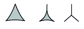
Figure 8: Hyperbolic triangle with increasing curvature (from left to right), the tree is the limit and a dimensional reduction 2D to 1D

10 Where do the Quantum Fluctuations Come From?

In a purely geometrical theory, one has to answer this question. It cannot be shifted to assume the appearance of quantum fluctuations. Instead we have to understand the root of these quantum fluctuations. Starting point of our approach is the foliation of the exotic $R^{4}$ by using the Anosov flow. Main point in the argumentation above is the appearance of the hyperbolic geometry in 3- and 4-dimensional submanifolds. The foliation can, however, be interpreted differently: a foliation defines a dynamics at a manifold leading to a splitting into leafs (the integral curves of the dynamics). Therefore, a tiny variation in the initial conditions will lead to a strong variation of the corresponding integral curve. This chaotic behavior is a natural consequence of the exotic smoothness structure (leading to the non-trivial $PSL(2,\mathbb{R})-$foliation). For completeness we will describe this dynamics, called the Anosov flow. For that purpose we consider the standard basis

$$J=\frac{1}{2}\left(\begin{array}[]{cc}1&0\\ 0&-1\end{array}\right)\quad,\,X=\left(\begin{array}[]{cc}0&1\\ 0&0\end{array}\right)\quad,\,Y=\left(\begin{array}[]{cc}0&0\\ 1&0\end{array}\right)$$ (23)

of the Lie algebra $sl(2,\mathbb{R})$ with

$$[J,X]=X\quad\quad[J,Y]=-Y\quad\quad[X,Y]=2J$$

leading to the exponential maps

$$g_{t}=\exp(tJ)=\left(\begin{matrix}e^{t/2}&0\\ 0&e^{-t/2}\end{matrix}\right)\,h_{t}^{*}=\exp(tX)=\left(\begin{matrix}1&t\\ 0&1\end{matrix}\right)\,h_{t}=\exp(tY)=\left(\begin{matrix}1&0\\ t&1\end{matrix}\right)$$

defining right-invariant flows on the unit tangent bundle $T_{1}\mathbb{H}=PSL(2,\mathbb{R})$ of the hyperbolic space. The connection to the Anosov flow comes from the realization that $g_{t}$ is the geodesic flow on $P=T_{1}\mathbb{H}$. With Lie vector fields being (by definition) left invariant under the action of a group element, one has that these fields are left invariant under the specific elements $g_{t}$ of the geodesic flow. This flow goes over to a surface $M=\mathbb{H}/\Gamma$ defined by a subgroup $\Gamma\subset PSL(2,\mathbb{R})$ with $Q=T_{1}M$. Now the geodesic flow $g_{t}$ acts on the exponential maps $g_{s},h_{t}^{*},h_{t}$ so that the geodesic flow itself is invariant, $g_{s}g_{t}=g_{t}g_{s}=g_{s+t}$ , but the other two shrink and expand: $g_{s}h_{t}^{*}=h_{t\cdot\exp(-s)}^{*}g_{s}$ and $g_{s}h_{t}=h_{t\cdot\exp(s)}g_{s}$. Then the bundle $TQ$ splits into three subbundles

$$TQ=E^{+}\oplus E^{0}\oplus E^{-}$$

where one bundle $E^{+}$ expands, one bundle $E^{-}$ contracts and one bundle $E^{0}$ is invariant w.r.t. geodesic flow. This property is crucial for the following discussion. Because of the expanding behavior of one subbundle, the Anosov flow is the generator of a chaotic dynamics. Therefore, two geodesics diverge exponentially in this foliation, but this behavior goes over to the holonomies characterizing the geometry. The transport of a holonomy along two diverging geodesics can lead to totally different holonomies. Currently this dynamics is deterministic, i.e. if we choose exactly the same initial condition then we will end at the state (seen as limit point). This situation changes if we are unable to choose the initial condition exactly (by choosing real numbers) but instead we can only choose a rational number where this rational number is the characterizing property of the state. Then all initial conditions (represented by all real numbers) in this class represent the same state but have totally different limit points of the corresponding dynamics. Now we will describe this dynamics.

Starting point is the observable algebra $X(S,SL(2,\mathbb{C})$, i.e. the space of holonomies $\pi_{1}(S)\to SL(2,\mathbb{C})$ (i.e. homomorphisms) up to conjugation, see subsection 6.3.1. The deformation quantization (see subsection 6.3.2) is the Kauffman bracket skein module. Here we made use of the identity

$$tr(A)\cdot tr(B)=tr(AB)+tr(AB^{-1})$$

between two elements $A,B\in SL(2,\mathbb{C})$ (w.r.t. a representation). Using the group commutator $[A,B]=ABA^{-1}B^{-1}$ one also obtains

$$2+tr([A,B])=(tr(A))^{2}+(tr(B))^{2}+(tr(AB))^{2}-tr(A)tr(B)tr(AB)$$

According to deformation procedure, pairs of elements $A,B\in SL(2,\mathbb{C})$ coming from closed curves via the holonomy and fulfilling

$$tr([A,B])=\pm 2$$

can be a canonical pair w.r.t. the symplectic structure. The sign is purely convention and we choose $tr([A,B])=-2$. Then the canonical pair has to fulfill the equation

$$(tr(A))^{2}+(tr(B))^{2}+(tr(AB))^{2}-tr(A)tr(B)tr(AB)=0$$

which can be written in a more familiar form

$$x^{2}+y^{2}+z^{2}-3xyz=0$$ (24)

by using $3x=tr(A),3y=tr(B),3z=tr(AB)$. Because of the discreteness of $\pi_{1}(S)$, we have to look for rational solutions of this equation (Diophantine equation). The solutions of the equation are Markoff triples forming a binary tree (see Fig. 9).

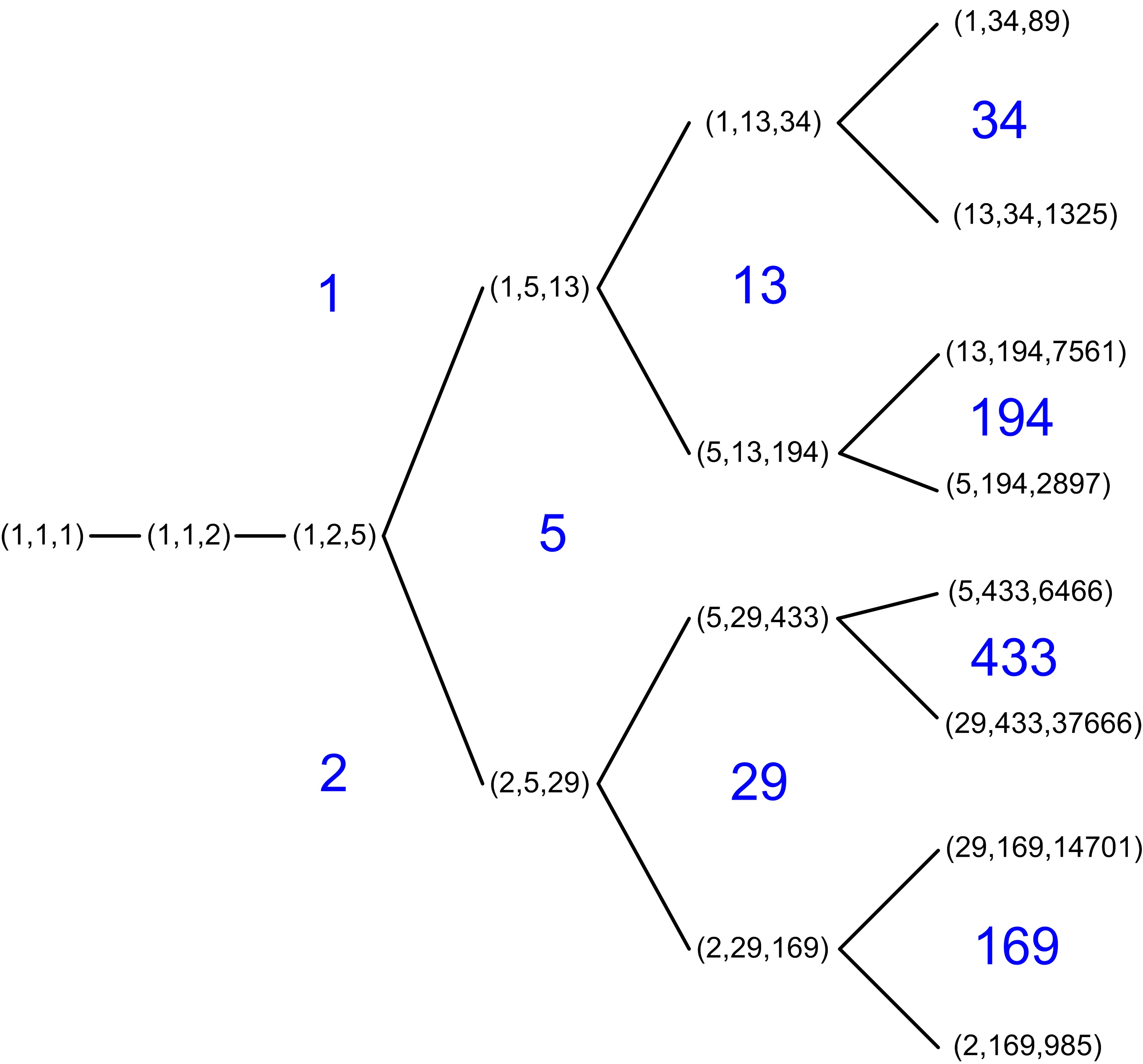
Figure 9: Binary tree of Markoff numbers as solution of equation (24).

The set of these elements $A,B$ corresponding to discrete groups is known to be fractal in nature [27]. It is the large class of quasi-Fuchsian groups having a fractal curve (Julia set) as limit set. Then we have the desired behavior:
The set of canonical pairs (as measurable variables in the theory) forms a fractal subset of the space of all holonomies. Then we can only determine the initial condition up to discrete value (given by the canonical pair) and the chaotic behavior of the foliation (i.e. the Anosov flow) makes the limit not predictable.
At the end of this section, one remark about the role of the canonical pair. It is always possible to construct a classical continuous random field that has the same probability density as the quantum vacuum state. Furthermore it is known that a random field can be generated by a chaotic dynamics. There is, however, a large difference between the classical random field and a quantum field: there are pairs of not equally accurate measurable observables (mostly the canonical pairs) for quantum fields impossible for the classical random fields. With our approach, we showed the same behavior for the canonical pairs.

11 Decoherence, Entanglement and Measurement

Our geometrical approach should also lead to a description of the measurement process (including the collapse of the wave function). In section 6, we constructed the geometrical expression for a quantum state given by a wild embedding (the wild $S^{3}$). The reduction of the quantum state (as linear combination) to an eigenstate (or the collapse of the wave function) is equivalent to a reduction of the wild embedding to a tame embedding. Therefore we need a mechanism to reduce the wild embedding to a tame one. The construction of the wild $S^{3}$ is strongly related to the Casson handle. The exoticness of the smooth structure of $R^{4}$ and the wildness of the $S^{3}$ depend both on the self-intersection of some disk. If we are able to remove these self-intersections then we will obtain the desired reduction. According to the discussion in subsection 3.2, one needs a Casson handle for the cancellation. How many levels of the Casson handle are needed to cancel the self-intersection? This question was answered by Freedman [54]: one needs three levels (a three-level Casson tower)! At the same time, however, one produces more self-intersections in the higher levels. Therefore one needs a little bit more: a Casson tower where a complete Casson handle can be embedded. Then this Casson handle is able to cancel the self-intersection and we will obtain a tame embedding or a classical state. As shown by Freedman [53] and Gompf/Singh [67], one needs a 5-stage Casson tower so that a Casson handle with the same attaching circle can be embedded into this 5-stage tower. We obtain a process which is ”the collapse of the wave function”. What is the cause of this collapse? As explained above, we cannot choose a single disk to remove the self-intersections. Instead we have to choose a Casson tower where each stage is a boundary-connected sum of $S^{1}\times D^{3}$, i.e. its boundary is the sum $S^{1}\times S^{2}\#S^{1}\times S^{2}\#\cdots$ where the number of components is equal to the number of self-intersections. So, every piece $S^{1}\times S^{2}$ of the boundary is given by the identification of the two boundary components for $S^{2}\times[0,1]$. In section 5, we identified this 3-manifold with the graviton or the collapse of the wave function is caused by a gravitational interaction. The corresponding process is known as decoherence. In the following we will calculate the minimal decoherence time for the gravitational interaction. The 5-stage Casson tower can be also understood as a cobordism between the 3-manifold

$$\Sigma_{0}=S^{1}\times S^{2}$$

(the $S^{1}$ defines the attaching circle) and a 3-manifold having the same homology. In case of the simplest Casson tower, it is given by five complements of the Whitehead link $C(Wh)$ closed by two solid tori, i.e.

$$\Sigma_{1}=(D^{2}\times S^{1})\cup C(Wh)\cup C(Wh)\cup C(Wh)\cup C(Wh)\cup C(Wh)\cup(D^{2}\times S^{1})$$

and this manifold can be very complicated for more complex towers. Now we will add some geometry to calculate the decoherence time. As shown by Witten [103, 104, 105], the action

$$\intop_{\Sigma_{0,1}}\,^{3}R\sqrt{h}\,d^{3}x=L\cdot CS(\Sigma_{0,1})$$ (25)

for every 3-manifold (in particular for $\Sigma_{0}$ and $\Sigma_{1}$ denoted by $\Sigma_{0,1}$) is related to the Chern-Simons action $CS(\Sigma_{0,1})$. The scaling factor $L$ is related to the volume by $L=\sqrt[3]{vol(\Sigma_{0,1})}$ and we obtain formally

$$L\cdot CS(\Sigma_{0,1},A)=L^{3}\cdot\frac{CS(\Sigma_{0,1})}{L^{2}}=\intop_{\Sigma_{0,1}}\frac{CS(\Sigma_{0,1})}{L^{2}\cdot vol(\Sigma_{0,1})}\sqrt{h}\,d^{3}x$$ (26)

by using

$$L^{3}\cdot vol(\Sigma_{0,1})=\intop_{\Sigma_{0,1}}\sqrt{h}\,d^{3}x$$

with the (unit) volume $vol(\Sigma_{0,1})$. If $\Sigma_{0,1}$ is a hyperbolic 3-manifold then the (unit) volume is a topological invariant which cannot be normalized to 1. Together with

$${}^{3}R=\frac{3k}{a^{2}}$$

one can compare the kernels of the integrals of (25) and (26) to get for a fixed time

$$\frac{3k}{a^{2}}=\frac{CS(\Sigma_{0,1})}{L^{2}\cdot vol(\Sigma_{0,1})}\,.$$

This gives the scaling factor

$$\vartheta=\frac{a^{2}}{L^{2}}=\frac{3\cdot vol(\Sigma_{0,1})}{CS(\Sigma_{0,1})}$$ (27)

where we set $k=1$ in the following. The hyperbolic geometry of the cobordism is best expressed by the metric

$$ds^{2}=dt^{2}-a(t)^{2}h_{ik}dx^{i}dx^{k}$$ (28)

also called the Friedmann-Robertson-Walker metric (FRW metric) with the scaling function $a(t)$ for the (spatial) 3-manifold. Mostow rigidity enforces us to choose

$$\left(\frac{\dot{a}}{a}\right)^{2}=\frac{1}{L^{2}}$$

in the length scale $L$ of the hyperbolic structure. In the following we will switch to quadratic expressions because we will determine the expectation value of the area. A second reason for the consideration of quadratic expressions is again the hyperbolic structure of $\mathbb{H}^{2}$. We needed this structure for the construction of the foliation which is given by a polygon in $\mathbb{H}^{2}$. This polygon defines a compact surface of genus $g>1$. Then the foliation of the polygon induces a foliation of the small exotic $R^{4}$. The area of the polygon is mainly the Godbillon-Vey invariant of the foliation. It is known that foliations of surfaces are given by quadratic differentials of the form defined below. Here, there are deep connections to trees and $SL(2,\mathbb{C})$ flat connections, i.e. a tree defines a quadratic differential and vice versa [90, 71, 106, 46].

Using the previous equation, we obtain

$$da^{2}=\frac{a^{2}}{L^{2}}\,dt^{2}=\vartheta\,dt^{2}$$ (29)

with respect to the scale $\vartheta$. By using the tree of the Casson handle, we obtain a countable infinite sum of contributions for (29). Before we start we will clarify the geometry of the Casson handle. A Casson handle admits a hyperbolic geometry. Therefore the tree corresponding to the Casson handle must be interpreted as a metric tree with hyperbolic structure in $\mathbb{H}^{2}$ and metric $ds^{2}=(dx^{2}+dy^{2})/y^{2}$. The embedding of the Casson handle in the cobordism is given by the rules

1. The direction of the increasing levels $n\to n+1$ is identified with $dy^{2}$ and $dx^{2}$ is the number of edges for a fixed level with scaling parameter $\vartheta$.

2. The contribution of every level in the tree is determined by the previous level best expressed in the scaling parameter $\vartheta$.

3. An immersed disk at level $n$ needs at least one disk to resolve the self-intersection point. This disk forms the level $n+1$ but this disk is connected to the previous disk. So we obtain for $da^{2}|_{n+1}$ at level $n+1$

   $$da^{2}|_{n+1}\sim\vartheta\cdot da^{2}|_{n}$$

   up to a constant.

By using the metric $ds^{2}=(dx^{2}+dy^{2})/y^{2}$ with the embedding ($y^{2}\to n+1$, $dx^{2}\to\vartheta$) we obtain for the change $dx^{2}/y^{2}$ along the $x-$direction (i.e. for a fixed $y$) $\frac{\vartheta}{n+1}$. This change determines the scaling from the level $n$ to $n+1$, i.e.

$$da^{2}|_{n+1}=\frac{\vartheta}{n+1}\cdot da^{2}|_{n}=\frac{\vartheta^{n+1}}{(n+1)!}\cdot da^{2}|_{0}$$

and after the whole summation (as substitute for an integral in case of discrete values) we obtain for the relative scaling

$$a^{2}=\sum_{n=0}^{\infty}\left(da^{2}|_{n}\right)=a_{0}^{2}\cdot\sum_{n=0}^{\infty}\frac{1}{n!}\vartheta^{n}=a_{0}^{2}\cdot\exp\left(\vartheta\right)=a_{0}^{2}\cdot l_{scale}$$ (30)

with $da^{2}|_{0}=a_{0}^{2}$. The Chern-Simons invariant for $\Sigma_{0}$ vanishes and we are left with

$$CS(\Sigma_{1})=\frac{5}{8}$$

and the complements $C(Wh)$ are hyperbolic 3-manifolds with

$$vol(\Sigma_{1})=5\cdot vol(C(Wh))\approx 18.31931...$$

by using the software Snapea. Finally for the scaling we obtain

$$\vartheta\approx 87.932688...$$

and for the time we have to choose

$$T_{decoherence}=T_{0}\cdot\exp\left(\frac{\vartheta}{2}\right)$$

using the well-known relation $a_{0}=cT_{0}$ between length and time, i.e. we see one coordinate along the Casson handle as time axis. The time $T_{0}$ has to be identified with the Planck time $T_{0}\approx 10^{-43}s$ (see section 5) so that

$$T_{decoherence}\approx 10^{-24}s$$

is the minimal decoherence time for the gravitational interaction.

Now we also discuss the entanglement which has to be also geometrically expressed. A quantum state is an element of the skein algebra $K_{t}(S)$ for $S\times[0,1]$. For two disjoint surfaces $S_{0}\sqcup S_{1}$ one has

$$K_{t}(S_{0}\sqcup S_{1})=K_{t}(S_{0})\otimes K_{t}(S_{1})\;.$$

Now let us choose a knot $|0\rangle$ in $S_{\text{0}}\times[0,1]$ as element of $K_{t}(S_{0})$ as well a knot $|1\rangle$ in $K_{t}(S_{1})$. Then $|0\rangle\otimes|1\rangle$ is an element of $K_{t}(S_{0}\sqcup S_{1})$. Furthermore we can assume that the knots $|1\rangle$ and $|0\rangle$ can be also an element of $K_{t}(S_{0})$ and $K_{t}(S_{1})$, respectively. Then the element

$$|0\rangle\otimes|1\rangle+|1\rangle\otimes|0\rangle$$

exists but now as an element of $K_{t}(S)$ with $S_{0}\sqcup S_{1}\subset S$. Using the skein relations in $K_{t}(S)$, see Fig. 7, we obtain a linking between the corresponding knots, i.e. $|0\rangle$ and $|1\rangle$ forming a link. Fig. 10 visualizes the transition from disjoint circles (=disjoint states) to linked circles (=entangled states).

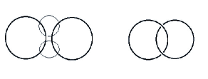
Figure 10: two disjoint circles get linked after the application of the skein relation for the area marked by the small circles

Then entanglement is reduced to a linking!

Next we have to think about the measurement which reduces the entangled state to one product state. Here we will only present some rough ideas for the description of the measurement process, but at first we have to define a measurement device. In this proposal, it is a union of Casson handles which can be used to unlink two linked components. At the level of skein algebras, the Casson handle is also given by elements of a skein algebra (given by closed, knotted curves at the levels). The particular structure of the Casson handle is not determined (see also section 10). Now a given quantum state is linked to this Casson handle. The limit point of the Casson handle (i.e. the leafs of the tree) give the result of the unlinking. All limit points of the Casson handle have a fractal structure (a Cantor set) expressing our inability to know the outcome of the measurement. The tree structure of the Casson handle has also another effect: the limit points are exponentially separated from each other and can be seen as classical states. With these speculations, we will close this section.

12 Some Implications for Cosmology

In the last section we will collect some implications for a cosmological model. Let us assume the topology $S^{3}\times\mathbb{R}$ for the spacetime but with an exotic smoothness structure $S^{3}\times_{\theta}\mathbb{R}$. One can construct this spacetime from the exotic $R^{4}$ by $R^{4}\setminus D^{4}=S^{3}\times_{\theta}\mathbb{R}$. From previous work, we know:

• Cosmological anomalies like dark matter and dark energy are (conjecturally) rooted in exotic smoothness [7].

• The initial state of the cosmos must be a wild 3-sphere representing a quantum state [16].

• Then there is an inflationary phase [18] driven by a decoherence which can be described by the Starobinsky model.
  In this model, we have a topological transition from a 3-manifold $\Sigma_{0}$ to another 3-manifold $\Sigma_{1}$. Both 3-manifolds are homology 3-spheres. Therefore let us describe this change (a so-called homology cobordism) between two homology 3-spheres $\Sigma_{0}$ and $\Sigma_{1}$. The situation can be described by a diagram

  $$\Sigma_{1} \stackrel{{\scriptstyle\Psi}}{{\longrightarrow}} \mathbb{R}$$

  $$\phi\downarrow \circlearrowright \updownarrow id$$ (31)

  $$\Sigma_{0} \stackrel{{\scriptstyle\psi}}{{\longrightarrow}} \mathbb{R}$$

  which commutes. The two functions $\psi$ and $\Psi$ are the Morse function of $\Sigma_{0}$ and $\Sigma_{1}$, respectively, with $\Psi=\psi\circ\phi$. The Morse function over $\Sigma_{0,1}$ is a function $\Sigma_{0,1}\to\mathbb{R}$ having only isolated, non-degenerated, critical points (i.e. with vanishing first derivatives at these points). A homology 3-sphere has two critical points (located at the two poles). The Morse function looks like $\pm||x||^{2}$ at these critical points. The transition $y=\phi(x)$ represented by the (homology) cobordism $M(\Sigma_{0},\Sigma_{1})$ maps the Morse function $\psi(y)=||y||^{2}$ on $\Sigma_{0}$ to the Morse function $\Psi(x)=||\phi(x)||^{2}$ on $\Sigma_{1}$. The function $-||\phi||^{2}$ represents also the critical point of the cobordism $M(\Sigma_{0},\Sigma_{1})$. As we learned above, this cobordism has a hyperbolic geometry and we have to interpret the function $||\phi(x)||^{2}$ not as an Euclidean form but change it to the hyperbolic geometry so that

  $$-||\phi||^{2}=-\left(\phi_{1}^{2}+\phi_{2}^{2}+\phi_{3}^{2}\right)\to-e^{-2\phi_{1}}(1+\phi_{2}^{2}+\phi_{3}^{2})$$

  i.e. we have a preferred direction represented by a single scalar field $\phi_{1}:\Sigma_{1}\to\mathbb{R}$. Therefore, the transition $\Sigma_{0}\to\Sigma_{1}$ is represented by a single scalar field $\phi_{1}:\Sigma_{1}\to\mathbb{R}$ and we identify this field as the moduli. Finally we interpret this Morse function in the interior of the cobordism $M(\Sigma_{0},\Sigma_{1})$ as the potential (shifted away from the point $0$ ) of the scalar field $\phi$ with Lagrangian

  $$L=R+(\partial_{\mu}\phi)^{2}-\frac{\rho}{2}(1-\exp\left(-\lambda\phi\right))^{2}$$

  with two free constants $\rho$ and $\lambda$. For the value $\lambda=\sqrt{2/3}$ and $\rho=3M^{2}$ we obtain the Starobinski model [89] (by a conformal transformation using $\phi$ and a redefinition of the scalar field [100])

  $$L=R+\frac{1}{6M^{2}}R^{2}$$ (32)

  with the mass scale $M\ll M_{P}$ much smaller than the Planck mass. From our discussion above, the appearance of this model is not totally surprising. It favors a surface to be incompressible (which is compatible with the properties of hyperbolic manifolds).

• This inflationary phase is followed by another exponentially increasing phase leading to a hyperbolic 4-manifold with constant curvature which is rigid by Mostow rigidity [18]. Here, we obtained the global geometry of the spacetime: it is a de Sitter space $SO(4,1)/SO(3,1)$ with a cosmological constant which is the curvature of the spacetime.

• This constant curvature can be identified with the cosmological constant in good agreement with the Planck satellite results [18]. The cosmological constant is constant by Mostow rigidity (but now for the 4-manifold).

• The topology of the spatial component (seen as 3-manifold) is strongly restricted [15] by the smoothness of the spacetime.

• The inclusion of matter can be done naturally as direct consequence of exotic smoothness [10].

• The interior of black holes can be described by exotic smoothness where the singularity is smoothed out [9].

13 Conclusion and Open Questions

Smooth Quantum Gravity, the usage of exotic smoothness structures on 4-manifolds, are the attempt to obtain a consistent theory of quantum gravity without any further assumptions. For us, the change of the smoothness structure is the next step in extending General Relativity, where non-Euclidean geometry was used to describe gravity and all accelerations. Then, two different smoothness structures represent two different physical systems. In particular I think that the standard smoothness structure represents the case of a spacetime without matter and non-gravitational fields. In this paper we are going a more radical way to construct a quantum theory without quantization but by using purely geometrical ideas from mathematical topics like differential and geometric topology. The flow of ideas can be simply described by the following points:

• An exotic $\mathbb{R}^{4}$ is given by an infinite handlebody (so one needs infinitely many charts) and one finds also the description by an infinite sequence of 3-manifolds together with 4-dimensional cobordisms connecting them.

• Every 3-manifold admits a codimension-one foliation which goes over to the 4-dimensional cobordisms. The leaf space of this foliation is an operator algebra with a strong connection to algebraic quantum field theory.

• The states (as linear functionals in the algebra) depend on knotted curves and are elements of the Kauffman bracket skein algebra. The reconstruction of the spatial space gives a wild embedded 3-sphere which is therefore related to the state, or the quantum state can be identified with the wild embedding. The classical state is a tame (i.e. usual) embedding where the deformation quantization of a tame embedding is a wild embedding.

• The structure of the operator algebra can be analyzed by the Tomita-Takesaki modular theory. Then it is possible to construct the quantum action by using the quantized calculus of Connes.

• For large scales, one gets the Einstein-Hilbert action. Whereas for small scales, one obtains a dimensional reduced action.

• The foliation is given by a hyperbolic dynamics having a chaotic behavior. For our states, one gets an unpredictable behavior so that the dynamics can generate the quantum fluctuations.

This list shows the current state but there are many open points, where we list only the most important here:

• What is the Hamiltonian of the theory? In principle we constructed this operator but have a problem connecting to Loop quantum gravity.

• What are the states seen as knots? The states are knots but the skein and Mandelstam identities give a class of knots: the states are conjecturally the concordance class of knots.

• Is the state a solution of the Hamiltonian? Here we conjecture that the concordance class of the knot lies already in the kernel of the Hamiltonian (therefore it is a solution of the Hamiltonian constraint)

A lot is done but there are also many open problems.
Happy Birthday Carl!

Appendix A Casson Handles and Labeled Trees

Let us now consider the basic construction of the Casson handle $CH$. Let $M$ be a smooth, compact, simply-connected 4-manifold and $f:D^{2}\to M$ a (codimension-2) mapping. By using diffeomorphisms of $D^{2}$ and $M$, one can deform the mapping $f$ to get an immersion (i.e. injective differential) generically with only double points (i.e. $\#|f^{-1}(f(x))|=2$) as singularities [62]. But to incorporate the generic location of the disk, one is rather interesting in the mapping of a 2-handle $D^{2}\times D^{2}$ induced by $f\times id:D^{2}\times D^{2}\to M$ from $f$. Then every double point (or self-intersection) of $f(D^{2})$ leads to self-plumbings of the 2-handle $D^{2}\times D^{2}$. A self-plumbing is an identification of $D_{0}^{2}\times D^{2}$ with $D_{1}^{2}\times D^{2}$ where $D_{0}^{2},D_{1}^{2}\subset D^{2}$ are disjoint sub-disks of the first factor disk. In complex coordinates the plumbing may be written as $(z,w)\mapsto(w,z)$ or $(z,w)\mapsto(\bar{w},\bar{z})$ creating either a positive or negative (respectively) double point on the disk $D^{2}\times 0$. Consider the pair $(D^{2}\times D^{2},\partial D^{2}\times D^{2})$ and produce finitely many self-plumbings away from the attaching region $\partial D^{2}\times D^{2}$ to get a kinky handle $(k,\partial^{-}k)$ where $\partial^{-}k$ denotes the attaching region of the kinky handle. A kinky handle $(k,\partial^{-}k)$ is a one-stage tower $(T_{1},\partial^{-}T_{1})$ and an $(n+1)$-stage tower $(T_{n+1},\partial^{-}T_{n+1})$ is an $n$-stage tower union of kinky handles $\bigcup_{\ell=1}^{n}(T_{\ell},\partial^{-}T_{\ell})$ where two towers are attached along $\partial^{-}T_{\ell}$. Let $T_{n}^{-}$ be $(\mbox{interior}T_{n})\cup\partial^{-}T_{n}$ and the Casson handle

$$CH=\bigcup_{\ell=0}T_{\ell}^{-}$$

is the union of towers (with direct limit topology induced from the inclusions $T_{n}\hookrightarrow T_{n+1}$). A Casson handle is specified up to (orientation preserving) diffeomorphism (of pairs) by a labeled finitely-branching tree with base-point *, having all edge paths infinitely extendable away from *. Each edge should be given a label $+$ or $-$ and each vertex corresponds to a kinky handle; the self-plumbing number of that kinky handle equals the number of branches leaving the vertex. The sign on each branch corresponds to the sign of the associated self plumbing. The whole process generates a tree with infinite many levels. In principle, every tree with a finite number of branches per level realizes a corresponding Casson handle. The simplest non-trivial Casson handle is represented by the tree $Tree_{+}$: each level has one branching point with positive sign $+$. The reverse construction of a Casson handle $CH_{\mathcal{T}}$ by using a labeled tree $\mathcal{T}$ can be found in the appendix A. Let $\mathcal{T}_{1}$ and $\mathcal{T}_{2}$ be two trees with $\mathcal{T}_{1}\subset\mathcal{T}_{2}$ (it is the subtree) then $CH_{\mathcal{T}_{2}}\subset CH_{\mathcal{T}_{1}}$.Given a labeled based tree $Q$, let us describe a subset $U_{Q}$ of $D^{2}\times D^{2}$. Now we will construct a $(U_{Q},\partial D^{2}\times D^{2})$ which is diffeomorphic to the Casson handle associated to $Q$. In $D^{2}\times D^{2}$ embed a ramified Whitehead link with one Whitehead link component for every edge labeled by $+$ leaving * and one mirror image Whitehead link component for every edge labeled by $-$(minus) leaving *. Corresponding to each first level node of $Q$ we have already found a (normally framed) solid torus embedded in $D^{2}\times\partial D^{2}$. In each of these solid tori embed a ramified Whitehead link, ramified according to the number of $+$ and $-$ labeled branches leaving that node. We can do that process for every level of $Q$. Let the disjoint union of the (closed) solid tori in the $n$-th family (one solid torus for each branch at level $n$ in $Q$) be denoted by $X_{n}$. $Q$ tells us how to construct an infinite chain of inclusions:

$$\ldots\subset X_{n+1}\subset X_{n}\subset X_{n-1}\subset\ldots\subset X_{1}\subset D^{2}\times\partial D^{2}$$

and we define the Whitehead decomposition $WhC_{Q}=\bigcap_{n=1}^{\infty}X_{n}$ of $Q$. $WhC_{Q}$ is the Whitehead continuum [99] for the simplest unbranched tree. We define $U_{Q}$ to be

$$U_{Q}=D^{2}\times D^{2}\setminus(D^{2}\times\partial D^{2}\cup\mbox{closure}(WhC_{Q}))$$

alternatively one can also write

$$U_{Q}=D^{2}\times D^{2}\setminus\mbox{cone}(WhC_{Q})$$ (33)

where $\mbox{cone}()$ is the cone of a space

$$cone(A)=A\times[0,1]/(x,0)\sim(x^{\prime},0)\qquad\forall x,x^{\prime}\in A$$

over the point $(0,0)\in D^{2}\times D^{2}$. As Freedman (see [53] Theorem 2.2) showed $U_{Q}$ is diffeomorphic to the Casson handle $CH_{Q}$ given by the tree $Q$.

Appendix B Thurston Foliation of a 3-Manifold

In [94] Thurston constructed a foliation of the 3-sphere $S^{3}$ which depends on a polygon $P$ in the hyperbolic plane $\mathbb{H}^{2}$ so that two foliations are non-cobordant if the corresponding polygons have different areas. For later usage, we will present the main ideas of this construction only (see also the book [92] chapter VIII for the details). Starting point is the hyperbolic plane $\mathbb{H}^{2}$ with a convex polygon $K\subset\mathbb{H}^{2}$ having $k$ sides $s_{1},\ldots,s_{k}$. Assuming the upper half plane model of $\mathbb{H}^{2}$ then the sides are circular arcs. The construction of the foliation depends mainly on the isometry group $PSL(2,\mathbb{R})$ of $\mathbb{H}^{2}$ realized as rational transformations (and this group can be lifted to $SL(2,\mathbb{R})$). The followings steps are needed in the construction:

1. The polygon $K$ is doubled along one side, say $s_{1}$, to get a polygon $K^{\prime}$. The sides are identified by (isometric) transformations $s_{i}\to s_{i}^{\prime}$ (as elements of $SL(2,\mathbb{R})$).

2. Take $\epsilon$-neighborhoods $U_{\epsilon}(p_{i}),U_{\epsilon}(p_{i}^{\prime})$ with $\epsilon>0$ sufficient small and set

   $$V^{2} =\left(K\cup K^{\prime}\right)\setminus\bigcup_{i=1}^{k}\left(U_{\epsilon}(p_{i})\cup U_{\epsilon}(p_{i}^{\prime})\right)$$

   $$=S^{2}\setminus\bigcup_{i=1}^{k}D_{i}^{2}$$

   having the topology of $V^{2}=S^{2}\setminus\left\{k\,\mbox{punctures}\right\}$ and we set $P=K\cup K^{\prime}$.

3. Now consider the unit tangent bundle $U\mathbb{H}^{2}$, i.e. a $S^{1}-$bundle over $\mathbb{H}^{2}$ (or the tangent bundle where every vector has norm one). The restricted bundle over $V^{2}$ is trivial so that $UV^{2}=V^{2}\times S^{1}$. Let $L,L^{\prime}$ be circular arcs (geodesics) in $\mathbb{H}^{2}$ (invariant w.r.t. $SL(2,\mathbb{R})$) starting at a common point which define parallel tangent vectors w.r.t. the metrics of the upper half plane model. The foliation of $V^{2}$ is given by geodesics transverse to the boundary and we obtain a foliation of $V^{2}\times S^{1}$ (as unit tangent bundle). This foliation is given by a $SL(2,\mathbb{R})$-invariant smooth 1-form $\omega$ (so that $\omega=const.$defines the leaves) which is integrable $d\omega\wedge\omega=0$. ($SL(2,\mathbb{R})-$invariant Foliation $\mathcal{F}_{SL}$)

4. With the relation $D^{2}=V^{2}\cup D_{1}^{2}\cup\cdots\cup D_{k-1}^{2}$, we obtain $D^{2}\times S^{1}=V^{2}\times S^{1}\cup\left(D_{1}^{2}\times S^{1}\right)\cup\cdots\cup\left(D_{k-1}^{2}\times S^{1}\right)$ or the gluing of $k-1$ solid tori to $V^{2}\times S^{1}$ gives a solid tori. Every glued solid torus will be foliated by a Reeb foliation. Finally using $S^{3}=(D^{2}\times S^{1})\cup(S^{1}\times D^{2})$ (the Heegard decomposition of the 3-sphere) again with a solid torus with Reeb foliation, we obtain a foliation on the 3-sphere.

The construction of this foliation $\mathcal{F}_{Thurston}$ (Thurston foliation) will be also work for any 3-manifold. Thurston [94] obtains for the Godbillon-Vey number

$$GV(V^{2}\times S^{1},\mathcal{F}_{SL})=4\pi\cdot vol(P)=8\pi\cdot vol(K)$$

and

$$GV(S^{3},\mathcal{F}_{Thurston})=4\pi\cdot Area(P)$$ (34)

so that any real number can be realized by a suitable foliation of this type. Furthermore, two cobordant foliations have the same Godbillon-Vey number (but the reverse is in general wrong). Let $[1]\in H^{3}(S^{3},\mathbb{R})$ be the dual of the fundamental class $[S^{3}]$ defined by the volume form, then the Godbillon-Vey class can be represented by

$$\Gamma_{\mathcal{F}_{a}}=4\pi\cdot Area(P)[1]$$ (35)

The Godbillon-Vey class is an element of the deRham cohomology $H^{3}(S^{3},\mathbb{R})$. Now we will discuss the general case of a compact 3-manifold carrying a foliation of the same type like the 3-sphere above. The main idea of the construction is very simple and uses a general representation of all compact 3-manifolds by Dehn surgery. Here we will use an alternative representation of surgery by using the Dehn-Lickorish theorem ([81] Corollary 12.4 at page 84). Let $\Sigma$ be a compact 3-manifold without boundary. There is now a natural number $k\in\mathbb{N}$ so that any orientable 3-manifold can be obtained by cutting out $k$ solid tori from the 3-sphere $S^{3}$ and then pasting them back in, but along different diffeomorphisms of their boundaries. Moreover, it can be assumed that all these solid tori in $S^{3}$ are unknotted. Then any 3-manifold $\Sigma$ can be written as

$$\Sigma=\left(S^{3}\setminus\left(\bigsqcup_{i=1}^{k}D_{i}^{2}\times S^{1}\right)\right)\cup_{\phi_{1}}\left(D_{1}^{2}\times S^{1}\right)\cup_{\phi_{2}}\cdots\cup_{\phi_{k}}\left(D_{k}^{2}\times S^{1}\right)$$

where $\phi_{i}:\partial\left(S^{3}\setminus\left(\bigsqcup_{i=1}^{k}D_{i}^{2}\times S^{1}\right)\right)\to\partial D_{i}^{2}\times S^{1}$ is the gluing map from each boundary component of $\left(S^{3}\setminus\left(\bigsqcup_{i=1}^{k}D_{i}^{2}\times S^{1}\right)\right)$ to the boundary of $\partial D_{i}^{2}\times S^{1}$. This gluing map is a diffeomorphism of tori $T^{2}\to T^{2}$ (where $T^{2}=S^{1}\times S^{1}$). The Dehn-Lickorish theorem describes all diffeomorphisms of a surface: Every diffeomorphism of a surface is the composition of Dehn twists and coordinate transformations (or small diffeomorphisms). The decomposition

$$S^{3}=\left(V^{2}\times S^{1}\right)\cup\left(D_{1}^{2}\times S^{1}\right)\cup\cdots\cup\left(D_{k-1}^{2}\times S^{1}\right)\cup\left(S^{1}\times D_{k}^{2}\right)$$ (36)

of the 3-sphere can be used to get a decomposition of $\Sigma$ by

$$\Sigma=\left(V^{2}\times S^{1}\right)\cup_{\phi_{1}}\left(D_{1}^{2}\times S^{1}\right)\cup_{\phi_{2}}\cdots\cup_{\phi_{k}}\left(D_{k}^{2}\times S^{1}\right)$$

which will guide us to the construction of a foliation on $\Sigma$:

• Construct a foliation $\mathcal{F}_{\Sigma,SL}$ on $V^{2}\times S^{1}$ using a polygon $P$ (see above) and

• Glue in $k$ Reeb foliations of the solid tori using the diffeomorphisms $\phi_{i}$.

Finally we get a foliation $\mathcal{F}_{\Sigma,Thurston}$ on $\Sigma$. According to the rules above, we are able to calculate the Godbillon-Vey number

$$GV(\Sigma,\mathcal{F}_{\Sigma,Thurston})=4\pi\cdot vol(P)$$

Therefore for any foliation of $S^{3}$, we can construct a foliation on any compact 3-manifold $\Sigma$ with the same Godbillon-Vey number. Both foliations $\mathcal{F}_{Thurston}$ and $\mathcal{F}_{\Sigma,Thurston}$ agree for the common submanifold $V^{2}\times S^{1}$ or there is a foliated cobordism between $V^{2}\times S^{1}\subset\Sigma$ and $V^{2}\times S^{1}\subset S^{3}$. Of course, $S^{3}$ and $\Sigma$ differ by the gluing of the solid tori but every solid torus carries a Reeb foliation which does not contribute to the Godbillon-Vey number.

Appendix C 3-Manifolds and Geometric Structures

A connected 3-manifold $N$ is prime if it cannot be obtained as a connected sum of two manifolds $N_{1}\#N_{2}$ neither of which is the 3-sphere $S^{3}$ (or, equivalently, neither of which is the homeomorphic to $N$). Examples are the 3-torus $T^{3}$ and $S^{1}\times S^{2}$ but also the Poincare sphere. According to [77], any compact, oriented 3-manifold is the connected sum of a unique (up to homeomorphism) collection of prime 3-manifolds (prime decomposition). A subset of prime manifolds are the irreducible 3-manifolds. A connected 3-manifold is irreducible if every differentiable submanifold $S$ homeomorphic to a sphere $S^{2}$ bounds a subset $D$ (i.e. $\partial D=S$) which is homeomorphic to the closed ball $D^{3}$. The only prime but reducible 3-manifold is $S^{1}\times S^{2}$. For the geometric properties (to meet Thurstons geometrization theorem) we need a finer decomposition induced by incompressible tori. A properly embedded connected surface $S\subset N$ is called 2-sided if its normal bundle is trivial, and 1-sided if its normal bundle is nontrivial. A 2-sided connected surface $S$ other than $S^{2}$ or $D^{2}$ is called incompressible if for each disk $D\subset N$ with $D\cap S=\partial D$ there is a disk $D^{\prime}\subset S$ with $\partial D^{\prime}=\partial D$. The boundary of a 3-manifold is an incompressible surface. Most importantly, the 3-sphere $S^{3}$, $S^{2}\times S^{1}$ and the 3-manifolds $S^{3}/\Gamma$ with $\Gamma\subset SO(4)$ a finite subgroup do not contain incompressible surfaces. The class of 3-manifolds $S^{3}/\Gamma$ (the spherical 3-manifolds) include cases like the Poincare sphere ($\Gamma=I^{*}$ the binary icosaeder group) or lens spaces ($\Gamma=\mathbb{Z}_{p}$ the cyclic group). Let $K_{i}$ be irreducible 3-manifolds containing incompressible surfaces then we can $N$ split into pieces (along embedded $S^{2}$)

$$N=K_{1}\#\cdots\#K_{n_{1}}\#_{n_{2}}S^{1}\times S^{2}\#_{n_{3}}S^{3}/\Gamma\,,$$ (37)

where $\#_{n}$ denotes the $n$-fold connected sum and $\Gamma\subset SO(4)$ is a finite subgroup. The decomposition of $N$ is unique up to the order of the factors. The irreducible 3-manifolds $K_{1},\ldots,\,K_{n_{1}}$ are able to contain incompressible tori and one can split $K_{i}$ along the tori into simpler pieces $K=H\cup_{T^{2}}G$ [73] (called the JSJ decomposition). The two classes $G$ and $H$ are the graph manifold $G$ and the hyperbolic 3-manifold $H$ (see Figure 11).

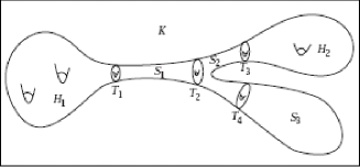
Figure 11: Torus (JSJ-) decomposition, $H_{i}$ hyperbolic manifold, $S_{i}$ Graph-manifold, $T_{i}$ Tori.

The hyperbolic 3-manifold $H$ has a torus boundary $T^{2}=\partial H$, i.e. $H$ admits a hyperbolic structure in the interior only. In this paper we need the splitting of the link/knot complement. As shown in [33], the Whitehead double of a knot leads to JSJ decomposition of the complement into the knot complement and the complement of the Whitehead link (along one torus boundary of the Whitehead link complement).

One property of hyperbolic 3-manifolds is central: Mostow rigidity. As shown by Mostow [78], every hyperbolic $n-$manifold $n>2$ with finite volume has this property: Every diffeomorphism (especially every conformal transformation) of a hyperbolic $n-$manifold with finite volume is induced by an isometry. Therefore one cannot scale a hyperbolic 3-manifold and the volume is a topological invariant. Together with the prime and JSJ decomposition

$$N=\left(H_{1}\cup_{T^{2}}G_{1}\right)\#\cdots\#\left(H_{n_{1}}\cup_{T^{2}}G_{n_{1}}\right)\#_{n_{2}}S^{1}\times S^{2}\#_{n_{3}}S^{3}/\Gamma\,,$$

we can discuss the geometric properties central to Thurstons geometrization theorem: Every oriented closed prime 3-manifold can be cut along tori (JSJ decomposition), so that the interior of each of the resulting manifolds has a geometric structure with finite volume. Now, we have to clarify the term geometric structure’s. A model geometry is a simply connected smooth manifold $X$ together with a transitive action of a Lie group $G$ on $X$ with compact stabilizers. A geometric structure on a manifold $N$ is a diffeomorphism from $N$ to $X/\Gamma$ for some model geometry $X$, where $\Gamma$ is a discrete subgroup of $G$ acting freely on $X$. t is a surprising fact that there are also a finite number of three-dimensional model geometries, i.e. 8 geometries with the following models: spherical $(S^{3},O_{4}(\mathbb{R}))$, Euclidean $(\mathbb{E}^{3},O_{3}(\mathbb{R})\ltimes\mathbb{R}^{3})$, hyperbolic $(\mathbb{H}^{3},O_{1,3}(\mathbb{R})^{+})$, mixed spherical-Euclidean $(S^{2}\times\mathbb{R},O_{3}(\mathbb{R})\times\mathbb{R}\times\mathbb{Z}_{2})$, mixed hyperbolic-Euclidean $(\mathbb{H}^{2}\times\mathbb{R},O_{1,3}(\mathbb{R})^{+}\times\mathbb{R}\times\mathbb{Z}_{2})$ and 3 exceptional cases called $\tilde{SL}_{2}$ (twisted version of $\mathbb{H}^{2}\times\mathbb{R}$), NIL (geometry of the Heisenberg group as twisted version of $\mathbb{E}^{3}$), SOL (split extension of $\mathbb{R}^{2}$ by $\mathbb{R}$, i.e. the Lie algebra of the group of isometries of 2-dimensional Minkowski space). We refer to [84] for the details.

References

- [1] H. Abchir. TQFT invariants at infinity for the Whitehead manifold. In C. McA. Gordan, V.F.R. Jones, L. Kauffman, S. Lambropoulou, and J.H. Przytycki, editors, Knots in Hellas ’98, pages 1–17, Singapore, 1998. World Scientific.
- [2] S. Akbulut and R. Kirby. Mazur manifolds. Mich. Math. J., 26:259–284, 1979.
- [3] A. Ashtekar, J. Engle, and D. Sloan. Asymptotics and Hamiltonians in a first order formalism. Class. Quant. Grav., 25:095020, 2008. arXiv:0802.2527.
- [4] A. Ashtekar and D. Sloan. Action and Hamiltonians in higher dimensional general relativity: First order framework. Class.Quant.Grav., 25:225025, 2008. arXiv:0808.2069.
- [5] T. Asselmeyer. Generation of source terms in general relativity by differential structures. Class. Quant. Grav., 14:749 – 758, 1996.
- [6] T. Asselmeyer-Maluga. Exotic smoothness and quantum gravity. Class. Q. Grav., 27:165002, 2010. arXiv:1003.5506.
- [7] T. Asselmeyer-Maluga and C.H. Brans. Cosmological anomalies and exotic smoothness structures. Gen. Rel. Grav., 34:1767–1771, 2002.
- [8] T. Asselmeyer-Maluga and C.H. Brans. Exotic Smoothness and Physics. WorldScientific Publ., Singapore, 2007.
- [9] T. Asselmeyer-Maluga and C.H. Brans. Smoothly Exotic Black Holes, pages 139–156. Space Science, Exploration and Policies. NOVA publishers, 2012.
- [10] T. Asselmeyer-Maluga and C.H. Brans. How to include fermions into general relativity by exotic smoothness. Gen. Relativ. Grav., 47:30, 2015. DOI 10.1007/s10714-015-1872-x, arXiv: 1502.02087.
- [11] T. Asselmeyer-Maluga and J. Król. Exotic smooth , noncommutative algebras and quantization. arXiv: 1001.0882, 2010.
- [12] T. Asselmeyer-Maluga and J. Król. Small exotic smooth and string theory. In International Congress of Mathematicians ICM 2010 Short Communications Abstracts Book, Ed. R. Bathia, page 400, Hindustan Book Agency, 2010.
- [13] T. Asselmeyer-Maluga and J. Król. Constructing a quantum field theory from spacetime. arXiv:1107.3458, 2011.
- [14] T. Asselmeyer-Maluga and J. Król. Topological quantum d-branes and wild embeddings from exotic smooth . Int. J. Mod. Phys., A26:3421 – 3437, 2011. arXiv:1105.1557.
- [15] T. Asselmeyer-Maluga and J. Król. On topological restrictions of the spacetime in cosmology. Mod. Phys. Lett. A, 27:1250135, 2012. arXiv:1206.4796.
- [16] T. Asselmeyer-Maluga and J. Król. Quantum geometry and wild embeddings as quantum states. Int. J. of Geometric Methods in Modern Physics, 10(10), 2013. will be published in Nov. 2013, arXiv:1211.3012.
- [17] T. Asselmeyer-Maluga and J. Król. Abelian gerbes, generalized geometries and foliations of small exotic . arXiv: 0904.1276v5, subm. to Rev. Math. Phys., 2014.
- [18] T. Asselmeyer-Maluga and J. Król. Inflation and topological phase transition driven by exotic smoothness. Advances in HEP, Article ID 867460:14 pages, 2014. http://dx.doi.org/10.1155/2014/867460.
- [19] T. Asselmeyer-Maluga and R. Mader. Exotic and quantum field theory. In C. Burdik Et. Al., editor, 7th International Conference on Quantum Theory and Symmetries (QTS7), page 012011, Bristol, UK, 2012. IOP Publishing. arXiv:1112.4885, doi:10.1088/1742-6596/343/1/012011.
- [20] T. Asselmeyer-Maluga and H. Rosé. On the geometrization of matter by exotic smoothness. Gen. Rel. Grav., 44:2825 – 2856, 2012. DOI: 10.1007/s10714-012-1419-3, arXiv:1006.2230.
- [21] N. Berline, M. Vergne, and E. Getzler. Heat kernels and Dirac Operators. Springer Verlag, New York, 1992.
- [22] P. Bertozzini, R. Conti, and W. Lewkeeratiyutkul. Modular theory, non-commutative geometry and quantum gravity. SIGMA, 6:47pp., 2010. arXiv:1007.4094.
- [23] Z. Bizaca. An explicit family of exotic Casson handles. Proc. AMS, 123:1297 – 1302, 1995.
- [24] Z̆. Biz̆aca and R Gompf. Elliptic surfaces and some simple exotic ’s. J. Diff. Geom., 43:458–504, 1996.
- [25] H.J. Borchers. On revolutionizing quantum field theory with Tomita’s modular theory. J. Math. Phys., 41:3604 – 3673, 2000.
- [26] R. Bott and L.W. Tu. Differential Forms in Algebraic Topology. Graduate Texts in Mathematics 82. Springer-Verlag, 1995.
- [27] B.H. Bowditch. Markoff triples and quasifuchsian groups. Proc. London Math. Soc., 77:697–736, 1998.
- [28] C. Branciard. How -epistemic models fail at explaining the indistinguishability of quantum states. Phys. Rev. Lett., 113:020409, 2014. DOI: 10.1103/PhysRevLett.113.020409.
- [29] C. Brans. Absolulte spacetime: the twentieth century ether. Gen. Rel. Grav., 31:597, 1999.
- [30] C.H. Brans. Exotic smoothness and physics. J. Math. Phys., 35:5494–5506, 1994.
- [31] C.H. Brans. Localized exotic smoothness. Class. Quant. Grav., 11:1785–1792, 1994.
- [32] C.H. Brans and D. Randall. Exotic differentiable structures and general relativity. Gen. Rel. Grav., 25:205, 1993.
- [33] R. Budney. JSJ-decompositions of knot and link complements in the 3-sphere. L’enseignement Mathématique, 52:319–359, 2006. arXiv:math/0506523.
- [34] D. Bullock. A finite set of generators for the Kauffman bracket skein algebra. Math. Z., 231:91–101, 1999.
- [35] D. Bullock, C. Frohman, and J. Kania-Bartoszyńska. Topological interpretations of lattice gauge field theory. Comm. Math. Phys., 198:47–81, 1998. arXiv:q-alg/9710003.
- [36] D. Bullock, C. Frohman, and J. Kania-Bartoszyńska. Understanding the Kauffman bracket skein module. J. Knot theory and Its Ramification, 8:265–277, 1999. arXiv: q-alg/9604013.
- [37] D. Bullock, C. Frohman, and J. Kania-Bartoszyńska. The Kauffman bracket skein as an algebra of observables. Proc. AMS, 130:2479–2485, 2002. arXiv:math/0010330.
- [38] D. Bullock and J.H. Przytycki. Multiplicative structure of Kauffman bracket skein module quantization. Proc. AMS, 128:923–931, 1999.
- [39] A. Casson. Three lectures on new infinite constructions in 4-dimensional manifolds, volume 62. Birkhäuser, progress in mathematics edition, 1986. Notes by Lucian Guillou, first published 1973.
- [40] V. Chernov and S. Nemirovski. Smooth cosmic censorship. Comm. Math. Phys., 320 (2013) 469-473 arXiv:1201.6070.
- [41] Fermi GBM/LAT Collaborations. Testing Einstein’s special relativity with Fermi’s short hard gamma-ray burst GRB090510. Nature, 462:331–334, 2009. arXiv:0908.1832.
- [42] A. Connes. A survey of foliations and operator algebras. Proc. Symp. Pure Math., 38:521–628, 1984. see www.alainconnes.org.
- [43] A. Connes. Non-commutative geometry. Academic Press, 1994.
- [44] A. Connes and C. Rovelli. Von neumann algebra automorphisms and time-thermodynamics relation in general covariant quantum theories. Class. Quant. Grav., 11:2899–2918, 1994. arXiv:gr-qc/9406019.
- [45] M. Culler and P.B. Shalen. Varieties of group representations and splittings of 3-manifolds. Ann. of Math., 117:109–146, 1983.
- [46] G. Daskalopoulos, S. Dostoglou, and R. Wentworth. Character varieties and harmonic maps to -trees. Math. Res. Lett., 5:523–533, 1998.
- [47] S. DeMichelis and M.H. Freedman. Uncountable many exotic ’s in standard 4-space. J. Diff. Geom., 35:219–254, 1992.
- [48] S. Donaldson. An application of gauge theory to the topology of 4-manifolds. J. Diff. Geom., 18:279–315, 1983.
- [49] S. Donaldson. Irrationality and the h-cobordism conjecture. J. Diff. Geom., 26:141–168, 1987.
- [50] C. Duston. Exotic smoothness in 4 dimensions and semiclassical Euclidean quantum gravity. Int.J.Geom.Meth.Mod.Phys., 8:459–484, 2010. arXiv: 0911.4068.
- [51] R. Fintushel and R. Stern. Knots, links, and 4-manifolds. Inv. Math, 134:363–400, 1998. (dg-ga/9612014).
- [52] A. Floer. An instanton invariant for 3-manifolds. Comm. Math. Phys., 118:215–240, 1988.
- [53] M.H. Freedman. The topology of four-dimensional manifolds. J. Diff. Geom., 17:357 – 454, 1982.
- [54] M.H. Freedman. The disk problem for four-dimensional manifolds. In Proc. Internat. Cong. Math. Warzawa, volume 17, pages 647 – 663, 1983.
- [55] M.H. Freedman. There is no room to spare in four-dimensional space. Noticess Amer. Math. Soc., 31:3–6, 1984.
- [56] D. Friedan. Nonlinear models in dimensions. Phys. Rev. Lett., 45:1057–1060, 1980.
- [57] T. Friedrich. On the spinor representation of surfaces in euclidean 3-space. J. Geom. and Phys., 28:143–157, 1998. arXiv:dg-ga/9712021v1.
- [58] C. Frohman and R. Gelca. Skein modules and the noncommutative torus. Trans. AMS, 352:4877–4888, 2000. arXiv:math/9806107.
- [59] S. Ganzell. Ends of 4-manifolds. Top. Proc., 30:223–236, 2006. aviable also at http://faculty.smcm.edu/sganzell/ends.pdf.
- [60] D. Gabai. Foliations and the Topology of 3-Manifolds. J. Diff. Geom., 18: 445-503, 1983.
- [61] W.M. Goldman. The symplectic nature of the fundamental groups of surfaces. Adv. Math., 54:200–225, 1984.
- [62] M. Golubitsky and V. Guillemin. Stable Mappings and their Singularities. Graduate Texts in Mathematics 14. Springer Verlag, New York-Heidelberg-Berlin, 1973.
- [63] R. Gompf. Infinite families of casson handles and topological disks. Topology, 23:395–400, 1984.
- [64] R Gompf. An infinite set of exotic ’s. J. Diff. Geom., 21:283–300, 1985.
- [65] R. Gompf. Periodic ends and knot concordance. Top. Appl., 32:141–148, 1989.
- [66] R.E. Gompf. Three exotic ’s and other anomalies. J. Diff. Geom., 18:317–328, 1983.
- [67] R.E. Gompf and S. Singh. On Freedman’s reimbedding theorems. In C. Gordan and R. Kirby, editors, Four-Manifold Theory, volume 35, pages 277–310, Providence Rhode Island, 1984. AMS, AMS.
- [68] R.E. Gompf and A.I. Stipsicz. 4-manifolds and Kirby Calculus. American Mathematical Society, 1999.
- [69] S.W. Hawking. The path-integral approach to quantum gravity. In Israel Hawking, editor, General Relativity. An Einstein Centenary Survey, pages 746–789, Cambridge, 1979. Cambridge University Press.
- [70] M. W. Hirsch. Differential Topology. Springer-Verlag, New York, 1976.
- [71] J. Hubbard and H. Masur. Quadratic differentials and foliations. Acta Math., 142:221–274, 1979.
- [72] S. Hurder and A. Katok. Secondary classes and trasnverse measure theory of a foliation. Bull. AMS, 11:347 – 349, 1984. announced results only.
- [73] W. Jaco and P. Shalen. Seifert fibered spaces in 3-manifolds, volume 21 of Mem. Amer. Math. Soc. AMS, 1979.
- [74] T. Kato. ASD moduli space over four-manifolds with tree-like ends. Geom. Top., 8:779 – 830, 2004. arXiv:math.GT/0405443.
- [75] M.S. Leifer. Is the quantum state real? an extended review of -ontology theorems. Quanta, 3:67–155, 2014. DOI: 10.12743/quanta.v3i1.22.
- [76] J. Mather. Stability of Mappings. VI: The nice dimensions. In Proccedings of the Liverpool Singularities Symposium, pages 207 – 253. Springer Lecture Notes in Mathematyics, Vol. 192, 1971.
- [77] J. Milnor. A unique decomposition theorem for 3-manifolds. Amer. J. Math., 84:1–7, 1962.
- [78] G.D. Mostow. Quasi-conformal mappings in -space and the rigidity of hyperbolic space forms. Publ. Math. IHÉS, 34:53–104, 1968.
- [79] R. Penrose. Nonlinear gravitons and curved twistor theory. Gen. Relativ. Grav., 7:31–52, 1976.
- [80] H. Pfeiffer. Quantum general relativity and the classification of smooth manifolds. Report number: DAMTP 2004-32, 2004.
- [81] V.V. Prasolov and A.B. Sossinisky. Knots, Links, Braids and 3-Manifolds. AMS, Providence, 1997.
- [82] B.L. Reinhart and J.W. Wood. A metric formula for the Godbillon-Vey invariant for foliations. Proc. AMS, 38:427–430, 1973.
- [83] M. Ringbauer, B. Duffus, C. Branciard, E. G. Cavalcanti, A. G. White, and A. Fedrizzi. Measurements on the reality of the wavefunction. Nature Physics, 11:249–254, 2015. DOI: 10.1038/NPHYS3233.
- [84] P. Scott. The geometries of 3-manifolds. Bull. London Math. Soc., 15:401–487, 1983.
- [85] A.R. Skovborg. The Moduli Space of Flat Connections on a Surface Poisson Structures and Quantization. PhD thesis, Universty Aarhus, 2006.
- [86] J. Sładkowski. Strongly gravitating empty spaces. Preprint gr-qc/9906037, 1999.
- [87] J. Sładkowski. Gravity on exotic with few symmetries. Int.J. Mod. Phys. D, 10:311–313, 2001.
- [88] J. Stallings. Piecewise-linear structure of euclidean space. Proc. Cambridge Phil. Soc., 58:481, 1962.
- [89] A.A. Starobinski. A new type of isotropic cosmological models without singularity. Phys. Lett., 91B:99–102, 1980.
- [90] K. Strebel. Quadratic Differentials. A Series of Modern Surveys in Math. Vol. Springer, Berlin-Heidelberg, 1984.
- [91] M. Takesaki. Tomita’s Theory of Modular Hilbert Algebras and its Applications. Lecture Notes in Mathematics, Vol. 128. Springer, Berlin - New York, 1970.
- [92] I. Tamura. Topology of Foliations: An Introduction. Translations of Math. Monographs Vol. 97. AMS, Providence, 1992.
- [93] C.H. Taubes. Gauge theory on asymptotically periodic 4-manifolds. J. Diff. Geom., 25:363–430, 1987.
- [94] W. Thurston. Noncobordant foliations of . Bull. AMS, 78:511 – 514, 1972.
- [95] W. Thurston. Three-Dimensional Geometry and Topology. Princeton University Press, Princeton, first edition, 1997.
- [96] M. Tomita. On canonical forms of von neumann algebras. In Fifth Functional Analysis Sympos (Tôhoku Univ., Sendai, 1967), pages 101–102, Sendai, 1967. Tôhoku Univ., Math. Inst.
- [97] V. Turaev. Algebras of loops on surfaces, algebras of knots, and quantization. Adv. Ser. Math. Phys., 9:59–95, 1989.
- [98] V.G. Turaev. Skein quantization of poisson algebras of loops on surfaces. Ann. Sci. de l’ENS, 24:635–704, 1991.
- [99] J. H. C. Whitehead. A certain open manifold whose group is unity. Quart. J. Math. Oxford, 6:268–279, 1935.
- [100] B. Whitt. Fourth order gravity as general relativity plus matter. Phys. Lett., 145B:176–178, 1984.
- [101] D.K. Wise. Symmetric space Cartan connections and gravity in three and four dimensions. SIGMA, 5:080, 2009. arXiv:0904.1738.
- [102] D.K. Wise. Macdowell-Mansouri gravity and Cartan geometry. Class. Quantum Grav., 27:155010, 2010. arXiv:gr-qc/0611154.
- [103] E. Witten. 2+1 dimensional gravity as an exactly soluble system. Nucl. Phys., B311:46–78, 1988/89.
- [104] E. Witten. Topology-changing amplitudes in 2+1 dimensional gravity. Nucl. Phys., B323:113–140, 1989.
- [105] E. Witten. Quantization of Chern-Simons gauge theory with complex gauge group. Comm. Math. Phys., 137:29–66, 1991.
- [106] M. Wolf. Harmonic maps from surfaces to -trees. Math. Z., 218:577–593, 1995.