On Layered Erasure Interference Channels without CSI at Transmitters

Abstract

This paper studies a layered erasure model for two-user interference channels, which can be viewed as a simplified version of Gaussian fading interference channel. It is assumed that channel state information (CSI) is only available at receivers but not at transmitters. Under such assumption, an outer bound is derived for the capacity region of such interference channel. The new outer bound is tight in many circumstances. For the remaining open cases, the outer bound extends previous results in [1].

I Introduction

Since the breakthrough of Gaussian interference channel by Etkin, Tse and Wang [2], the study of interference networking has made plenty of progress[3]. However, most works still focus on situations where channel state information (CSI) is static and known to both transmitters (CSIT) and receivers (CSIR). These results usually valid under situations where CSI variates slowly and systems have efficient sounding and feedback mechanisms to update global CSI timely. For communications experiencing fast channel fading, we usually do not have such luxury to have (accurate and timely) CSI at transmitters.

In this paper, we investigate a layered erasure model of two-user interference channel (IC), which shares the same spirit as deterministic model used in [4], except that the transmit binary vectors are erased randomly. We assume that the erasure levels (which model the fading states or CSI) are known at the receivers but not at transmitters. In particular, we derive an outer bound for general two-user layered erasure interference channels with no CSI at transmitters. The obtained new bound is generally tight for many important cases but whether it is tight for all situations is still open in this paper. Comparing with previous results in [1], this paper can be viewed as a fully extension to multi-layer situations.

The remaining paper is organized as following. In next section, the channel model is formally described and some notation is introduced to assist the further discussion. In Section III, our main finding is presented and followed by several remarks to clarify the new outer bound. We continue our discussion by investigating some non-trivial situations in Section IV. Limited by the space, we only present a brief proof of the outer bound in Section V. Finally, we conclude this paper in Section VI.

II Model and Notations

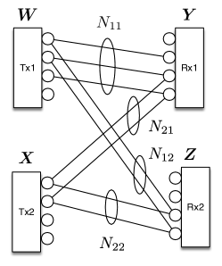
Figure 1: Layered Erasure Interference Channel Model.

Consider a layered erasure interference channel as shown in Fig. 1. At each time $i$, transmitters 1 and 2 emit binary-vector signals $\boldsymbol{W}[i]$ and $\boldsymbol{X}[i]$, respectively, which take value in $\mathbb{F}^{q}_{2}$. Only a certain top portion of each vector signal reaches the two receivers, and the remaining part is erased randomly. Mathematically, let $\boldsymbol{\underline{s}}$ denote a $q\times q$ matrix whose elements are all $0$ except that $\boldsymbol{\underline{s}}_{k+1,k}=1$ for $k=1,\dots,q-1$. It is easy to see that $\boldsymbol{\underline{s}}[x_{1},x_{2},\dots,x_{q}]^{\mathsf{T}}=[0,x_{1},\dots,x_{q-1}]^{\mathsf{T}}$, and $\boldsymbol{\underline{s}}^{q-n}[x_{1},x_{2},\dots,x_{q}]^{\mathsf{T}}=[0,\dots,0,x_{1},\dots,x_{n}]^{\mathsf{T}}$, which is equivalent to a zero-padding downward shift of the vector so that only its first $n$ elements are left. With these notations, at each time $i$, the two received signals, $\boldsymbol{Y}[i]$ and $\boldsymbol{Z}[i]$, can be written as,

$$\boldsymbol{Y}[i] =\boldsymbol{\underline{s}}^{q-N_{11}[i]}\boldsymbol{W}[i]\oplus\boldsymbol{\underline{s}}^{q-N_{21}[i]}\boldsymbol{X}[i]$$ (1a)

$$\boldsymbol{Z}[i] =\boldsymbol{\underline{s}}^{q-N_{12}[i]}\boldsymbol{W}[i]\oplus\boldsymbol{\underline{s}}^{q-N_{22}[i]}\boldsymbol{X}[i],$$ (1b)

respectively, where for $t,r=1,2$, each integer random process $\{N_{tr}[i]\}$ models the channel fading process from transmitter $t$ to receiver $r$. We assume that the four fading processes are independent of each other and each of them is independent and identically distributed (i.i.d) over time (so that the channel is memoryless). In this paper, we study situations where receiver 1 knows realization of $(N_{11}[i],N_{21}[i])$ and receiver 2 knows realization of $(N_{22}[i],N_{12}[i])$ at each time $i$, but no channel state information (CSI) is available at both transmitters except for the statistical law of those fading processes.

For remaining discussion, we need following notations. Suppose $\boldsymbol{X}\in\mathbb{F}^{q}_{2}$ is an arbitrary random vector. We use $X_{j}$ to denote its $j$-th element and $\boldsymbol{X}_{j}^{k}$ to denote its sub-vector $[X_{j},\dots,X_{k}]^{\mathsf{T}}$. For the special case where subscript $j=1$, we often use $\boldsymbol{X}^{k}$ instead of $\boldsymbol{X}^{k}_{1}$. We often use lower-case letters to denote realizations of their corresponding random vectors or random variables. For example, $\boldsymbol{x}=[x_{1},x_{2},\dots,x_{q}]^{\mathsf{T}}$ should be interpreted as a particular realization of the random vector $\boldsymbol{X}$. For any sequence of random vectors $\{\boldsymbol{X}[i]\}$, let $(\boldsymbol{X})_{i_{1}}^{i_{2}}$ denote the subsequence $\boldsymbol{X}[i_{1}],\dots,\boldsymbol{X}[i_{2}]$. Consequently, $(\boldsymbol{X}_{j}^{k})_{i_{1}}^{i_{2}}$ denotes the subsequence $\boldsymbol{X}_{j}^{k}[i_{1}],\boldsymbol{X}_{j}^{k}[i_{1}+1],\dots,\boldsymbol{X}_{j}^{k}[i_{2}]$. In summary, the indices outside the parentheses always refer to time while inside ones refer to element(s) of the corresponding vectors. Binary addition ($\oplus$) between two vectors with different lengths is aligned at the least significant bits: if $n_{1}\geq n_{2}$, then define $\boldsymbol{X}^{n_{1}}\oplus\boldsymbol{W}^{n_{2}}=[X_{1},\dots,X_{n_{1}-n_{2}},X_{n_{1}-n_{2}+1}\oplus W_{1},\dots,X_{n_{1}}\oplus W_{n_{2}}]^{\mathsf{T}}$. Since we only consider memoryless channels in this paper, we often surpress the time index $i$ to ease the notations. For example, $\mathsf{P}\left(N_{11}\geq l\right)$ is equivalent to $\mathsf{P}\left(N_{11}[i]\geq l\right)$, distribution of $N_{11}[i]$ is referred as distribution of $N_{11}$, et al.With the convention introduced above, channel model (1) can be rewritten as

$$\boldsymbol{Y} =\boldsymbol{W}^{N_{11}}\oplus\boldsymbol{X}^{N_{21}}$$ (2a)

$$\boldsymbol{Z} =\boldsymbol{W}^{N_{12}}\oplus\boldsymbol{X}^{N_{22}}.$$ (2b)

III Main Results

Our main findings are summarized in Theorem 1, which needs a few of more definitions. Define following three regions within first orthant of $\mathbb{R}^{2}$ as

$$\mathcal{R}_{1a} :=\bigcap_{\omega\in[0,1]}\left\{\left.(R_{1},R_{2})\in\mathbb{R}^{2}_{\geq 0}\right|R_{1}+\omega R_{2}\leq\mathsf{B}_{1a}(\omega)\right\}$$ (3a)

$$\mathcal{R}_{1b} :=\bigcap_{\omega\in[0,1]}\left\{\left.(R_{1},R_{2})\in\mathbb{R}^{2}_{\geq 0}\right|R_{1}+\omega R_{2}\leq\mathsf{B}_{1b}(\omega)\right\}$$ (3b)

$$\mathcal{R}_{1c} :=\bigcap_{\begin{subarray}{c}\mu\in[0,\omega]\\ \omega\in[0,1]\end{subarray}}\left\{\left.(R_{1},R_{2})\in\mathbb{R}^{2}_{\geq 0}\right|(1+\mu)R_{1}+\omega R_{2}\leq\mathsf{B}_{1c}(\omega,\mu)\right\}$$ (3c)

where

$$\mathsf{B}_{1a}(\omega)=\mathbb{E}N_{11}+\omega\mathbb{E}\left[N_{21}-N_{11}\right]^{+}+\sum_{l=1}^{q}\left[\omega\beta_{1}(l)-\alpha_{1}(l)\right]^{+},$$ (4a)

$$\mathsf{B}_{1b}(\omega)\leq(1-\omega)\mathbb{E}N_{11}+\omega\mathbb{E}N_{21}+\sum_{l=1}^{q}\left[\omega\gamma_{1}(l)-\alpha_{1}(l)\right]^{+}+\omega\sum_{l=1}^{q}\max\big{(}\mathsf{P}\left(N_{11}-N_{21}\geq l\right),\mathsf{P}\left(N_{12}\geq l\right)\big{)},$$ (4b)

$$\mathsf{B}_{1c}(\omega,\mu)=\mathbb{E}N_{11}+\omega\mathbb{E}\left[N_{21}-N_{11}\right]^{+}+\sum_{l=1}^{q}\left[\omega\gamma_{1}(l)-\alpha_{1}(l)\right]^{+}+\sum_{l=1}^{q}\max\left(\mu\mathsf{P}\left(N_{11}\geq l\right),\omega\mathsf{P}\left(N_{12}\geq l\right)\right),$$ (4c)

and

$$\alpha_{1}(l) =\mathsf{P}\left(N_{21}\geq l\right)-\mathsf{P}\left(N_{21}-N_{11}\geq l\right),$$ (5a)

$$\beta_{1}(l) =\big{[}\mathsf{P}\left(N_{22}\geq l\right)-\mathsf{P}\left(N_{21}-N_{11}\geq l\right)\big{]}^{+}$$ (5b)

$$\gamma_{1}(l) =\big{[}\mathsf{P}\left(N_{22}-N_{12}\geq l\right)-\mathsf{P}\left(N_{21}-N_{11}\geq l\right)\big{]}^{+}.$$ (5c)

By swapping subscripts $1$ and $2$ in (5), we can define $\alpha_{2}(l)$, $\beta_{2}(l)$, and $\gamma_{2}(l)$ accordingly. For example, $\alpha_{2}(l):=\mathsf{P}\left(N_{12}\geq l\right)-\mathsf{P}\left(N_{12}-N_{22}\geq l\right)$. In turn, we can define $\mathsf{B}_{2j}$ and $\mathcal{R}_{2j}$ for $j\in\{a,b,c\}$ by exchanging subscripts $1$ with $2$ in (3) and (4).

Theorem 1

The capacity region $\mathcal{C}$ of the two-user interference channel (1) is contained in $\mathcal{R}_{1a}\cap\mathcal{R}_{1b}\cap\mathcal{R}_{1c}\cap\mathcal{R}_{2a}\cap\mathcal{R}_{2b}\cap\mathcal{R}_{2c}$.

To help understand the outer bound, we make following remarks.

Remark 1

Each region $\mathcal{R}_{kj}$, where $k\in\{1,2\}$ and $j\in\{a,b,c\}$, is a convex region characterized by a set of weighted sum-rate bounds, which is associated with each $\mathsf{B}_{kj}$. Although the intersections are done among infinite numbers of $\omega$ and $\mu$ in (3), it is not difficult to see that only finite numbers of them are necessary. Therefore, each $\mathcal{R}_{kj}$ is a polytope. In the remaining discussion, we refer to the weighted bound of form $R_{1}+\omega R_{2}\leq\mathsf{B}_{1a}(\omega)$ as bound $\mathsf{B}_{1a}(\omega)$, and $(1+\mu)R_{1}+\omega R_{2}\leq\mathsf{B}_{1c}(\omega,\mu)$ as bound $\mathsf{B}_{1c}(\omega,\mu)$, et al., for each fixed $\omega$ and $\mu$. Furthermore, on the boundary of each region $\mathcal{R}_{1j}$ (inside the first orthant), $R_{1}$ has larger weight than $R_{2}$, which corresponds to a situation where rate of user 1 is preferred to that of user 2. By symmetry, similar interpretation can be made to each region $\mathcal{R}_{2j}$, where user 2 is the preferred one.

Remark 2

By setting each $\{N_{tr}[i]\}$, $t,r=1,2$, to a constant, say $n_{tr}$, the new outer bound recovers the capacity region of its deterministic counterpart, which consists of all positive rate pairs satisfying [5, 4]:

$$R_{r} \leq n_{rr}\quad r=1,2$$ (6a)

$$R_{1}+R_{2} \leq\max(n_{11},n_{21})+(n_{22}-n_{21})^{+}$$ (6b)

$$R_{1}+R_{2} \leq\max(n_{22},n_{12})+(n_{11}-n_{12})^{+}$$ (6c)

$$R_{1}+R_{2} \leq\max((n_{11}-n_{21})^{+},n_{12})+\max((n_{22}-n_{12})^{+},n_{21})$$ (6d)

$$2R_{1}+R_{2} \leq\max(n_{11},n_{12})+(n_{11}-n_{21})^{+}+\max((n_{22}-n_{12})^{+},n_{21})$$ (6e)

$$R_{1}+2R_{2} \leq\max(n_{22},n_{21})+(n_{22}-n_{12})^{+}+\max((n_{11}-n_{21})^{+},n_{12}).$$ (6f)

We leave the detailed proof in Appendix A. Table I is a brief summary of the proof and it also highlights the relation between each region $\mathcal{R}_{kj}$, $k=1,2$ and $j\in\{a,b,c\}$, and each constraint in (6). We will look into more sophisticated examples in Section IV.

Theorem 1	Constraint in (6)
$\mathsf{B}_{1a}(\omega)$ and $\mathsf{B}_{2a}(\omega)$ with $\omega=0$	(6a)
$\mathsf{B}_{1a}(\omega)$ with $\omega=1$	(6b)
$\mathsf{B}_{2a}(\omega)$ with $\omega=1$	(6c)
$\mathsf{B}_{1b}(\omega)$ or $\mathsf{B}_{2b}(\omega)$ with $\omega=1$	(6d)
$\mathsf{B}_{1c}(\omega,\mu)$ with $\omega=1,\mu=1$	(6e)
$\mathsf{B}_{2c}(\omega,\mu)$ with $\omega=1,\mu=1$	(6f)

TABLE I: A summary of how to obtain capacity region of the deterministic IC via Theorem 1. It also shows how each bound $\mathsf{B}_{kj}$, for $k=1,2$ and $j=\{a,b,c\}$, relates to each constraint of (6).

Remark 3

Regions $\mathcal{R}_{1a}$ and $\mathcal{R}_{2a}$ are actually capacity regions of Z-IC with $N_{21}\equiv 0$ and $N_{12}\equiv 0$, respectively [6]. The remaining four are new.

IV More Discussion: Layered Erasure Cases

In this section, we will investigate Theorem 1 under several special situations, which include cases where Theorem 1 is tight as well as some open cases. Inspired by classification done in [1] for $q=1$, we define following three cases:

1. Stochastically strong interference: $\forall l\in\{1,\dots,q\}$,

   $$\mathsf{P}\left(N_{12}\geq l\right) \geq\mathsf{P}\left(N_{11}\geq l\right)$$

   $$\mathsf{P}\left(N_{21}\geq l\right) \geq\mathsf{P}\left(N_{22}\geq l\right);$$

2. Stochastically weak interference: $\forall l\in\{1,\dots,q\}$,

   $$\mathsf{P}\left(N_{11}-N_{21}\geq l\right) \geq\mathsf{P}\left(N_{12}\geq l\right)$$

   $$\mathsf{P}\left(N_{22}-N_{12}\geq l\right) \geq\mathsf{P}\left(N_{21}\geq l\right);$$

3. Stochastically moderate interference: $\forall l\in\{1,\dots,q\}$,

   $$\mathsf{P}\left(N_{11}\geq l\right) >\mathsf{P}\left(N_{12}\geq l\right)>\mathsf{P}\left(N_{11}-N_{21}\geq l\right)$$ (9a)

   $$\mathsf{P}\left(N_{22}\geq l\right) >\mathsf{P}\left(N_{21}\geq l\right)>\mathsf{P}\left(N_{22}-N_{12}\geq l\right).$$ (9b)

The first case can be interpreted as following: from the viewpoint of any given layer $l$, signal reaches to the undesired user more often than the desired one, which is similar to the strong interference channels in usual sense [7]. Both of the other two cases implies that $\mathsf{P}\left(N_{12}\geq l\right)\leq\mathsf{P}\left(N_{11}\geq l\right)$ and $\mathsf{P}\left(N_{21}\geq l\right)\leq\mathsf{P}\left(N_{22}\geq l\right)$ for any $l$. Therefore, they can be interpreted as cases where signal reaches to the desired user more often than the undesired one from the viewpoint of each layer. Hence, they both fall into weak interference category in usual sense.

In this section, we will show that the new outer bound actually coincides with the capacity regions for the first two cases. However, for the moderate interference case, whether Theorem 1 is tight still remains open. Note that general layered erasure channel can be much more complicated so that it can be none of these three cases. We will conclude this section with some discussion about general cases.

IV-A Stochastically Strong Interference

For strong interference, it is well known that the capacity region is the same as capacity region of compound multi-access channel at receivers 1 and 2 [7], i.e.,

$$\left\{(R_{1},R_{2})\in\mathbb{R}^{2}_{\geq 0}\left|\begin{array}[]{rcl}R_{i}&\leq&\mathbb{E}N_{rr}\quad r=1,2\\ R_{1}+R_{2}&\leq&\max\big{(}\mathbb{E}\max(N_{11},N_{21}),\mathbb{E}\max(N_{22},N_{12})\big{)}\end{array}\right\}.\right.$$ (12)

From Theorem 1, we see that all summation terms vanish in $\mathsf{B}_{kj}$, $k=1,2$ and $j\in\{a,b,c\}$ under stochastically strong interference assumption. Therefore, it is not difficult to see that the outer bound becomes $\mathcal{R}_{1a}\cap\mathcal{R}_{2a}$, which coincides with the region defined by (12).

IV-B Stochastically Weak Interference

Theorem 2

For interference channel which satisfies condition (8) $\forall$ $l\in\{1,\dots,q\}$, the capacity region is characterized by Theorem 1. In particular, it coincides with $\mathcal{R}_{1b}\cap\mathcal{R}_{2b}$ and sum-capacity is given by

$$C_{sum}=\mathbb{E}\left[N_{22}-N_{12}\right]^{+}+\mathbb{E}\left[N_{11}-N_{21}\right]^{+}.$$ (13)

Proof:

We start with the converse, which makes construction of achievable schemes more intuitive. Since (8) holds for any $l$, we can simplify $\mathsf{B}_{1b}(\omega)$ as

$$\mathsf{B}_{1b}(\omega) =(1-\omega)\mathbb{E}N_{11}+\omega\mathbb{E}N_{21}+\sum_{l=1}^{q}\left[\omega\gamma_{1}(l)-\alpha_{1}(l)\right]^{+}+\omega\sum_{l=1}^{q}\mathsf{P}\left(N_{11}-N_{21}\geq l\right)$$

$$=(1-\omega)\mathbb{E}N_{11}+\omega\mathbb{E}N_{21}+\sum_{l=1}^{q}\left[\omega\gamma_{1}(l)-\alpha_{1}(l)\right]^{+}+\omega\mathbb{E}\left[N_{11}-N_{21}\right]^{+}$$

$$=\mathbb{E}N_{11}+\omega\mathbb{E}\left[N_{21}-N_{11}\right]^{+}+\sum_{l=1}^{q}\left[\omega\gamma_{1}(l)-\alpha_{1}(l)\right]^{+}.$$ (14)

With (8) and (5b), we have $\beta_{1}(l)\geq\gamma_{1}(l)$. Therefore $\mathsf{B}_{1b}(\omega)\leq\mathsf{B}_{1a}(\omega)$ $\forall\omega\in[0,1]$, which implies $\mathcal{R}_{1b}\subset\mathcal{R}_{1a}$. For $\mathsf{B}_{1c}(\omega,\mu)$, we have

$$\mathsf{B}_{1c}(\omega,\mu) =\mathbb{E}N_{11}+\omega\mathbb{E}\left[N_{21}-N_{11}\right]^{+}+\sum_{l=1}^{q}\left[\omega\gamma_{1}(l)-\alpha_{1}(l)\right]^{+}$$

$$\quad+\sum_{l=1}^{q}\big{[}\max\big{(}\mu\mathsf{P}\left(N_{11}\geq l\right),\omega\mathsf{P}\left(N_{12}\geq l\right)\big{)}-\mu\mathsf{P}\left(N_{11}\geq l\right)+\mu\mathsf{P}\left(N_{11}\geq l\right)\big{]}$$

$$=(1+\mu)\mathbb{E}N_{11}+\omega\mathbb{E}\left[N_{21}-N_{11}\right]^{+}+\sum_{l=1}^{q}\left[\omega\gamma_{1}(l)-\alpha_{1}(l)\right]^{+}$$

$$\quad+\sum_{l=1}^{q}\left[\omega\mathsf{P}\left(N_{12}\geq l\right)-\mu\mathsf{P}\left(N_{11}\geq l\right)\right]^{+}.$$ (15)

Therefore, bound $\mathsf{B}_{1c}(\omega,\mu)$ can be rewritten as

$$R_{1}+\frac{\omega}{1+\mu}R_{2} \leq\mathbb{E}N_{11}+\frac{\omega}{1+\mu}\mathbb{E}\left[N_{21}-N_{11}\right]^{+}+\sum_{l=1}^{q}\left[\frac{\omega}{1+\mu}\gamma_{1}(l)-\frac{1}{1+\mu}\alpha_{1}(l)\right]^{+}$$

$$\quad+\sum_{l=1}^{q}\left[\frac{\omega}{1+\mu}\mathsf{P}\left(N_{12}\geq l\right)-\frac{\mu}{1+\mu}\mathsf{P}\left(N_{11}\geq l\right)\right]^{+}.$$ (16)

Comparing with (14), we see that the right-hand side (RHS) of (16) is greater or equals to $\mathsf{B}_{1b}(\frac{\omega}{1+\mu})$ for each fixed $\omega$ and $\mu$. Therefore, $\mathcal{R}_{1b}\subset\mathcal{R}_{1c}$. Hence, we have $\mathcal{R}_{1b}\subset\mathcal{R}_{1a}\bigcap\mathcal{R}_{1c}$. By symmetry, we can argue that $\mathcal{R}_{2b}\subset\mathcal{R}_{2a}\cap\mathcal{R}_{2c}$. Therefore, the outer bound in Theorem 1 equals to $\mathcal{R}_{1b}\cap\mathcal{R}_{2b}$ under the stochastically weak interference assumption.

Let $\omega=1$ in (14), we obtain

$$R_{1}+R_{2} \leq\mathbb{E}\max\big{(}N_{11},N_{21}\big{)}+\sum_{l=1}^{q}\left[\gamma_{1}(l)-\alpha_{1}(l)\right]^{+}.$$ (17)

With (5c) and (5a), we have

$$\gamma_{1}(l)-\alpha_{1}(l) =\big{[}\mathsf{P}\left(N_{22}-N_{12}\geq l\right)-\mathsf{P}\left(N_{21}-N_{11}\geq l\right)\big{]}^{+}-\mathsf{P}\left(N_{21}\geq l\right)+\mathsf{P}\left(N_{21}-N_{11}\geq l\right)$$

$$=\max\big{(}\mathsf{P}\left(N_{22}-N_{12}\geq l\right),\mathsf{P}\left(N_{21}-N_{11}\geq l\right)\big{)}-\mathsf{P}\left(N_{21}\geq l\right).$$

With condition (8), we have $\mathsf{P}\left(N_{22}-N_{12}\geq l\right)\geq\mathsf{P}\left(N_{21}\geq l\right)\geq\mathsf{P}\left(N_{21}-N_{11}\geq l\right)$. Therefore,

$$\gamma_{1}(l)-\alpha_{1}(l) =\mathsf{P}\left(N_{22}-N_{12}\geq l\right)-\mathsf{P}\left(N_{21}\geq l\right).$$ (18)

From condition (8) and equation (18), we observe that that $\gamma_{1}(l)-\alpha_{1}(l)\geq 0$ for any $l$. Substitute (18) into (17), we have $R_{1}+R_{2}\leq C_{sum}$.

By symmetry, we have shown that $\mathsf{B}_{1b}(1)=\mathsf{B}_{2b}(1)=C_{sum}$. In fact, it is not difficult to see that boundaries of $\mathcal{R}_{1b}$ and $\mathcal{R}_{2b}$ intersects inside the first orthant at point $(R_{1},R_{2})=$$(\mathbb{E}\left[N_{11}-N_{21}\right]^{+}$ , $\mathbb{E}\left[N_{22}-N_{12}\right]^{+})$. Indeed, this point can be achieved by treating interference as noise at both receivers. We illustrate $\mathcal{R}_{1b}$ and $\mathcal{R}_{2b}$ in Fig. 2 by shadowing them with blue and green, respectively. To show the overlapped region is achievale, it is sufficient to construct a coding scheme for each extreme point. Let us focus on one of them, say, point A in Fig. 2.

(14) holds some insights about the coding schemes. Note that $\big{(}\mathbb{E}N_{11},\mathbb{E}\left[N_{21}-N_{11}\right]^{+}\big{)}$ is always on the boundary of $\mathcal{R}_{1b}$, which marks by $\bigstar$ in Fig 2. If user 1 and user 2 transmit their information at rate $\mathbb{E}N_{11}$ and $\mathbb{E}\left[N_{21}-N_{11}\right]^{+}$, respectively, user 1’s rate is achievable by decoding and canceling user 2’s message completely. One the other hand, user 2 should not have issue to decode its message at rate of $\mathbb{E}\left[N_{21}-N_{11}\right]^{+}$ by treating user 1’s signal as noise, because $\mathbb{E}\left[N_{21}-N_{11}\right]^{+}\leq\mathbb{E}\left[N_{22}-N_{12}\right]^{+}$ by weak interference assumption. If user 2 would like to send at higher rate, it faces a tradeoff by generating more interference, which, consequently, will reduce user 1’s rate. This type of tradeoff is captured by the summation term in (14). Therefore an achievable scheme for point A can be constructed as following. Both users generate their codebooks according to the distribution of q-size random vector whose elements are all i.i.d. $\mathrm{Ber}\left(1/2\right)$ random variables. Here, $\mathrm{Ber}\left(p\right)$ denotes Bernoulli distribution with probability $p$ taking value $1$ and probability $1-p$ taking value $0$. To finalize the coding scheme, we only need to determine the allocation of layers for private and common messages, respectively, in the spirit of Han-kobayashi (HK) scheme.

Suppose that the right boundary segment of point A is on a line of form $R_{1}+\omega_{A}R_{2}=const.$ Let us define two subsets of $\{1,\dots,q\}$: $\mathcal{L}_{p}:=\{l|\omega_{A}\gamma_{1}(l)\geq\alpha_{1}(l)\}$ and $\mathcal{L}_{c}:=\{l|\omega_{A}\gamma_{1}(l)<\alpha_{1}(l)\}$. Thus, we can write the coordinate of point A as

$$\left(\mathbb{E}N_{11}-\sum_{l\in\mathcal{L}_{p}}\alpha_{1}(l)\,,\,\mathbb{E}\left[N_{21}-N_{11}\right]^{+}+\sum_{l\in\mathcal{L}_{p}}\gamma_{1}(l)\right).$$ (19)

In terms of coding scheme, we allocate all layers of user 1 for private message. For user 2, we allocate layers in $\mathcal{L}_{p}$ to carry private message and layers in $\mathcal{L}_{c}$ to carry common message. At receiving sides, receiver 1 decodes and removes common message of user 2 before decoding its own message. By evaluating the corresponding mutual information, one can verify that user 1 can achieve transmit rate at $\mathbb{E}N_{11}-\sum_{l\in\mathcal{L}_{p}}\alpha_{1}(l)$. On the other hand, we have

$$\mathbb{E}\left[N_{21}-N_{11}\right]^{+}+\sum_{l\in\mathcal{L}_{p}}\gamma_{1}(l)$$

$$= \mathbb{E}\left[N_{21}-N_{11}\right]^{+}+\sum_{l=1}^{q}\gamma_{1}(l)-\sum_{l\in\mathcal{L}_{c}}\gamma_{1}(l)$$

$$= \sum_{l=1}^{q}\max\big{(}\mathsf{P}\left(N_{22}-N_{12}\geq l\right),\mathsf{P}\left(N_{21}-N_{11}\geq l\right)\big{)}-\sum_{l\in\mathcal{L}_{c}}\gamma_{1}(l)$$

$$= \sum_{l=1}^{q}\mathsf{P}\left(N_{22}-N_{12}\geq l\right)-\sum_{l\in\mathcal{L}_{c}}\gamma_{1}(l)$$ (20)

$$\geq\mathbb{E}\left[N_{22}-N_{12}\right]^{+}$$ (21)

where (20) is due to weak interference assumption (8). By (21), we see that user 2 can decode its own message at rate $\mathbb{E}\left[N_{21}-N_{11}\right]^{+}+\sum_{l\in\mathcal{L}_{p}}\gamma_{1}(l)$ by treating interference from user 1 as noise. ∎

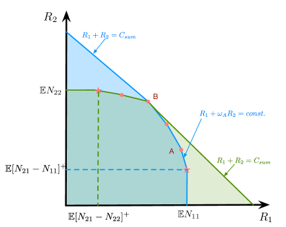
Figure 2: Sketch of capcity region of a weak interference channel. Regions with blue and green shadow are $\mathcal{R}_{1b}$ and $\mathcal{R}_{2b}$, respectively. Each of them is a polytope and their intersection is the capacity region. Point B is the intersection between boundaries of the two regions and it achieves the sum-capacity.

IV-C Stochastically Moderate Interference

Whether the outer bound given by Theorem 1 is also tight or not for moderate interference is not clear. But with condition (9), we can simply the bound further:

Proposition 1

For moderate interference channel, which satisfies condition (9) $\forall l$, we have

$$\mathsf{B}_{1a}(\omega)=\mathbb{E}N_{11}+\omega\mathbb{E}\left[N_{21}-N_{11}\right]^{+}+\sum_{l=1}^{q}\left[\omega\beta_{1}(l)-\alpha_{1}(l)\right]$$ (22a)

$$\mathsf{B}_{1b}(\omega)\leq(1-\omega)\mathbb{E}N_{11}+\omega\big{(}\mathbb{E}N_{21}+\mathbb{E}N_{12}\big{)}$$ (22b)

$$\mathsf{B}_{1c}(\omega,\mu)=\mathbb{E}N_{11}+\omega\mathbb{E}\left[N_{21}-N_{11}\right]^{+}+\sum_{l=1}^{q}\max\left(\mu\mathsf{P}\left(N_{11}\geq l\right),\omega\mathsf{P}\left(N_{12}\geq l\right)\right),$$ (22c)

and $$\mathsf{B}_{2a} \mathsf{B}_{2b} \mathsf{B}_{2c} 1 2$$, and are in similar forms with subscripts and exchanged, accordingly.

The proof is similar as reverse part of Theorem 2, except that with condition (9) we have $\gamma_{k}(l)<\alpha_{k}(l)$, for $k=1,2$ and $\forall l\in\{1,\dots,q\}$.

With $q=1$, Proposition 1 does not improve results for sum-rate obtained in [1]. However, it does provide a slightly better outer bound for the whole capacity region. To see this, we simplify the notation for symmetric single-layered case, i.e. $q=1$ as following. $\mathsf{P}\left(N_{11}=1\right)=\mathsf{P}\left(N_{22}=1\right)=p_{d}$ and $\mathsf{P}\left(N_{21}=1\right)=\mathsf{P}\left(N_{12}=1\right)=p_{c}$. The moderate interference assumption (9) becomes $p_{d}>p_{c}>\frac{p_{d}}{1+p_{d}}$, or, equivalently, $p_{d}p_{c}>p_{d}-p_{c}>0$. With these notations, we have

$$\alpha_{1}(1) =\alpha_{2}(1)=p_{d}p_{c}$$

$$\beta_{1}(1) =\beta_{2}(1)=p_{d}-p_{c}+p_{d}p_{c}$$

For $k=1,2$, consider $\mathsf{B}_{ka}(0)$, $\mathsf{B}_{ka}\left(\frac{\alpha_{1}(1)}{\beta_{1}(1)}\right)$, $\mathsf{B}_{kb}\left(1\right)$, and $\mathsf{B}_{kc}\left(1,\frac{p_{c}}{p_{d}}\right)$ accordingly. We obtain an outer bound as

$$\left\{(R_{1},R_{2})\in\mathbb{R}^{2}_{\geq 0}\left|\begin{array}[l]{rcl}R_{i}&\begin{subarray}{c}(a)\\ \leq\end{subarray}&p_{d}\quad i=1,2\\ R_{1}+\frac{p_{d}p_{c}}{p_{d}-p_{c}+p_{d}p_{c}}R_{2}&\begin{subarray}{c}(b)\\ \leq\end{subarray}&p_{d}+\frac{p_{d}p_{c}}{p_{d}-p_{c}+p_{d}p_{c}}p_{c}(1-p_{d})\\ \frac{p_{d}p_{c}}{p_{d}-p_{c}-p_{d}p_{c}}R_{1}+R_{2}&\begin{subarray}{c}(c)\\ \leq\end{subarray}&p_{d}+\frac{p_{d}p_{c}}{p_{d}-p_{c}+p_{d}p_{c}}p_{c}(1-p_{d})\\ R_{1}+R_{2}&\begin{subarray}{c}(d)\\ \leq\end{subarray}&2p_{c}\\ R_{1}+\frac{p_{d}}{p_{d}+p_{c}}R_{2}&\begin{subarray}{c}(e)\\ \leq\end{subarray}&p_{d}+\frac{p_{d}}{p_{d}+p_{c}}p_{c}(1-p_{d})\\ \frac{p_{d}}{p_{d}+p_{c}}R_{1}+R_{2}&\begin{subarray}{c}(f)\\ \leq\end{subarray}&p_{d}+\frac{p_{d}}{p_{d}+p_{c}}p_{c}(1-p_{d})\end{array}\right\}\right.$$ (29)

Note that conditions $(a)$–$(d)$ are shown in [1] and none of them is redundant when $p_{d}p_{c}>p_{d}-p_{c}>0$. We will show that in some condition $(e)$ is stronger than $(b)$. In fact, we observe that lines $R_{1}+\frac{p_{d}p_{c}}{p_{d}-p_{c}+p_{d}p_{c}}R_{2}=p_{d}+\frac{p_{d}p_{c}}{p_{d}-p_{c}+p_{d}p_{c}}p_{c}(1-p_{d})$ and $R_{1}+\frac{p_{d}}{p_{d}+p_{c}}R_{2}=p_{d}+\frac{p_{d}}{p_{d}+p_{c}}p_{c}(1-p_{d})$ intersect at $(p_{d},p_{c}(1-p_{d}))$. Regarding the slopes of these two lines, $\frac{p_{d}}{p_{d}+p_{c}}>\frac{p_{d}p_{c}}{p_{d}-(1-p_{d})p_{c}}$ under the condition of $p_{d}-p_{c}>p_{c}^{2}$. In other word, when $p_{d}-p_{c}>p_{c}^{2}$, $(b)$ becomes redundant to $(e)$. Note that $p_{d}-p_{c}>p_{c}^{2}$ can happen under moderate interference assumption.

IV-D General Cases

One can evaluate Theorem 1 under all kinds of different conditions beyond what we have discussed above. For example, one can mixed conditions of weak, moderate, strong interference between the two users. Moreover, in above three situations, we require (7), (8), or (9) hold for all $l$. One can also come up a case where conditions of (7), (8), and (9) are mixed across different layers. Therefore, structures of general layered erasure channels could be very complicated. However, we believe the limitation of Theorem 1 roots on our limited understanding of the moderate interference with $q=1$. In particular, we conjecture that

Conjecture 1

Theorem 1 characterizes the capacity region of general layered erasure channels, which satisfy condition that there does not exist $l\in\{1,\dots,q\}$ such that either (9a) or (9b) holds.

V Proof of Theorem 1

V-A Preliminary Lemmas

The proof relies on following two lemmas.

Lemma 1

Consider $n$ uses of a memoryless channel described by random transformation $\mathsf{P}_{Y,Z,T|X,S}$. Let $\boldsymbol{X}^{n}$ and $\boldsymbol{S}^{n}$ denote the independent input and state sequences, respectively. Then for any $\mu_{2}\geq\mu_{1}\geq 0$,

$$\mu_{1}\mathcal{I}\left(\boldsymbol{X}^{n};\boldsymbol{Z}^{n}|\boldsymbol{T}^{n},\boldsymbol{S}^{n}\right) -\mu_{2}\mathcal{I}\left(\boldsymbol{X}^{n};\boldsymbol{Y}^{n}|\boldsymbol{T}^{n},\boldsymbol{S}^{n}\right)$$

$$\leq\sum_{i=1}^{n}\Big{[}\mu_{1}\mathcal{I}\left(X_{i};Z_{i}|\boldsymbol{Z}^{i-1},\boldsymbol{Y}_{i+1}^{n},\boldsymbol{T}^{n},\boldsymbol{S}^{n}\right)-\mu_{2}\mathcal{I}\left(X_{i};Y_{i}|\boldsymbol{Z}^{i-1},\boldsymbol{Y}_{i+1}^{n},\boldsymbol{T}^{n},\boldsymbol{S}^{n}\right)\Big{]}.$$ (30)

It is a Marton-style expansion of mutual information, which essentially converts a multi-letter mutual information difference into a single-letter one. For the proof, please refer to [6, Appendix A] .

Lemma 2

Suppose that $(\boldsymbol{W})^{n}$ and $(\boldsymbol{X})^{n}$ are two independent arbitrary random processes taking value in $\mathbb{F}^{q}_{2}$. Let $(N_{1})^{n}$ and $(N_{2})^{n}$ be two i.i.d fading processes taking value in $\{0,\dots,q\}$. Then we have

$$\mathcal{I}\left(\left.(\boldsymbol{W})^{n},(\boldsymbol{X})^{n};(\boldsymbol{W}^{N_{1}}\oplus\boldsymbol{X}^{N_{2}})^{n}\right|(N_{1})^{n},(N_{2})^{n}\right)\leq n\mathbb{E}N_{1}+\mathcal{I}\left(\left.(\boldsymbol{X})^{n};(\boldsymbol{X}^{(N_{2}-N_{1})^{+}})^{n}\right|(N_{1})^{n},(N_{2})^{n}\right)$$ (31)

Proof:

$$\mathcal{I}\left(\left.(\boldsymbol{W})^{n},(\boldsymbol{X})^{n};(\boldsymbol{W}^{N_{1}}\oplus\boldsymbol{X}^{N_{2}})^{n}\right|(N_{1})^{n},(N_{2})^{n}\right)$$

$$= \mathcal{H}\left(\left.(\boldsymbol{W}^{N_{1}}\oplus\boldsymbol{X}^{N_{2}})^{n}\right|(N_{1})^{n},(N_{2})^{n}\right)$$

$$\leq \mathcal{H}\left(\left.(\boldsymbol{W}^{N_{1}}\oplus\widetilde{\boldsymbol{W}}^{N_{1}}\oplus\boldsymbol{X}^{N_{2}})^{n}\right|(N_{1})^{n},(N_{2})^{n}\right)$$

where $(\widetilde{\boldsymbol{W}})^{n}$ be an i.i.d. random sequence independent of all other random processes and each element of $\widetilde{\boldsymbol{W}}[i]$ is an independent $\mathrm{Ber}\left(1/2\right)$ random variable. Note that $(\widetilde{\boldsymbol{W}}\oplus\boldsymbol{W})^{n}$ has same distribution as $\widetilde{\boldsymbol{W}}$ and it is also independent of $(\boldsymbol{X})^{n}$. Let $\overline{\boldsymbol{W}}[i]=\widetilde{\boldsymbol{W}}[i]\oplus\boldsymbol{W}[i]$. Then

$$\mathcal{I}\left(\left.(\boldsymbol{W})^{n},(\boldsymbol{X})^{n};(\boldsymbol{W}^{N_{1}}\oplus\boldsymbol{X}^{N_{2}})^{n}\right|(N_{1})^{n},(N_{2})^{n}\right)$$

$$\leq \mathcal{H}\left(\left.(\overline{\boldsymbol{W}}^{N_{1}}\oplus\boldsymbol{X}^{N_{2}})^{n}\right|(N_{1})^{n},(N_{2})^{n}\right)$$

$$= \mathcal{I}\left(\left.(\overline{\boldsymbol{W}})^{n},(\boldsymbol{X})^{n};(\overline{\boldsymbol{W}}^{N_{1}}\oplus\boldsymbol{X}^{N_{2}})^{n}\right|(N_{1})^{n},(N_{2})^{n}\right)$$

$$= \mathbb{E}N_{1}+\mathcal{I}\left(\left.(\boldsymbol{X})^{n};(\overline{\boldsymbol{W}}^{N_{1}}\oplus\boldsymbol{X}^{N_{2}})^{n}\right|(N_{1})^{n},(N_{2})^{n}\right)$$ (32)

$$= \mathbb{E}N_{1}+\mathcal{I}\left(\left.(\boldsymbol{X})^{n};(\boldsymbol{X}^{(N_{2}-N_{1})^{+}})^{n},(\overline{\boldsymbol{W}}^{N_{1}}\oplus\boldsymbol{X}^{N_{1}})^{n}\right|(N_{1})^{n},(N_{2})^{n}\right).$$ (33)

where (32) is due to chain rule and (33) leads us to (31) by noting that $(\overline{\boldsymbol{W}}^{N_{1}}\oplus\boldsymbol{X}^{N_{1}})^{n}$ and $(\boldsymbol{X}^{(N_{2}-N_{1})^{+}})^{n}$ are independent of each other given $\left((N_{1})^{n},(N_{2})^{n}\right)$. ∎

Basically, Lemma 2 claims that for multi-access layered erasure channel, we can fix one input as $(\widetilde{\boldsymbol{W}})^{n}$ without reducing the sum-rate.

V-B Proof

First, by letting $N_{12}[i]\equiv 0$, we obtained a z-interference channel, whose capacity region can serve as a natural outer bound. Therefore, bounds $\mathsf{B}_{1a}(\omega)$ and $\mathsf{B}_{2a}(\omega)$ are direct consequence of [6, Theorem 2]. Thus, it is sufficient to show the remaining four bounds. By symmetry, we only need to show bounds $\mathsf{B}_{1b}$ and $\mathsf{B}_{1c}$, respectively.

For shorthand notation, we define $\boldsymbol{N}[i]=\big{(}N_{11}[i],N_{12}[i],N_{22}[i],N_{21}[i]\big{)}$. $\forall\omega\in[0,1]$, applying Fano’s inequality at receiver 1, we have

$$nR_{1}-n\delta_{n} \leq\mathcal{I}\left(\left.(\boldsymbol{W})^{n};(\boldsymbol{Y})^{n}\right|(\boldsymbol{N})^{n}\right)$$

$$=\mathcal{I}\left(\left.(\boldsymbol{W})^{n},(\boldsymbol{X})^{n};(\boldsymbol{Y})^{n}\right|(\boldsymbol{N})^{n}\right)-\mathcal{I}\left(\left.(\boldsymbol{X})^{n};(\boldsymbol{X}^{N_{21}})^{n}\right|(\boldsymbol{N})^{n}\right)$$ (34)

$$=\omega\mathcal{I}\left(\left.(\boldsymbol{W})^{n},(\boldsymbol{X})^{n};(\boldsymbol{Y})^{n}\right|(\boldsymbol{N})^{n}\right)+(1-\omega)\mathcal{I}\left(\left.(\boldsymbol{W})^{n},(\boldsymbol{X})^{n};(\boldsymbol{Y})^{n}\right|(\boldsymbol{N})^{n}\right)$$

$$\qquad-\mathcal{I}\left(\left.(\boldsymbol{X})^{n};(\boldsymbol{X}^{N_{21}})^{n}\right|(\boldsymbol{N})^{n}\right)$$

$$\leq\omega\mathcal{I}\left(\left.(\boldsymbol{W})^{n},(\boldsymbol{X})^{n};(\boldsymbol{Y})^{n}\right|(\boldsymbol{N})^{n}\right)+n(1-\omega)\mathbb{E}N_{11}+(1-\omega)\mathcal{I}\left(\left.(\boldsymbol{X})^{n};(\boldsymbol{X}^{(N_{21}-N_{11})^{+}})^{n}\right|(\boldsymbol{N})^{n}\right)$$

$$\qquad-\mathcal{I}\left(\left.(\boldsymbol{X})^{n};(\boldsymbol{X}^{N_{21}})^{n}\right|(\boldsymbol{N})^{n}\right)$$ (35)

where (34) is due to chain rule; in (35), we apply Lemma 2 by letting $N_{1}=N_{11}$ and $N_{2}=N_{21}$; and $\delta_{n}$ vanishes as $n\to\infty$.

Apply Fano’s inequality at receiver 2, we have

$$nR_{2}-n\delta_{n} \leq\mathcal{I}\left(\left.(\boldsymbol{X})^{n};(\boldsymbol{Z})^{n}\right|(\boldsymbol{N})^{n}\right)$$

$$=\mathcal{I}\left(\left.(\boldsymbol{W})^{n},(\boldsymbol{X})^{n};(\boldsymbol{Z})^{n}\right|(\boldsymbol{N})^{n}\right)-\mathcal{I}\left(\left.(\boldsymbol{W})^{n};(\boldsymbol{W}^{N_{12}})^{n}\right|(\boldsymbol{N})^{n}\right)$$ (36)

$$=\mathbb{E}N_{12}+\mathcal{I}\left(\left.(\boldsymbol{X})^{n};(\boldsymbol{X}^{(N_{22}-N_{12})^{+}})^{n}\right|(\boldsymbol{N})^{n}\right)-\mathcal{I}\left(\left.(\boldsymbol{W})^{n};(\boldsymbol{W}^{N_{12}})^{n}\right|(\boldsymbol{N})^{n}\right)$$ (37)

where (36) is due to chain rule and in (37), we apply Lemma with $N_{1}=N_{12}$ and $N_{2}=N_{22}$.

By combining (35) and (37), we can get a weighted bound:

$$n(R_{1} +\omega R_{2}-(1+\omega)\delta_{n})$$

$$\leq n(1-\omega)\mathbb{E}N_{11}+n\omega\mathbb{E}N_{12}+A+B$$ (38)

where

$$A =\omega\mathcal{I}\left(\left.(\boldsymbol{X})^{n};(\boldsymbol{X}^{(N_{22}-N_{12})^{+}})^{n}\right|(\boldsymbol{N})^{n}\right)-\mathcal{I}\left(\left.(\boldsymbol{X})^{n};(\boldsymbol{X}^{N_{21}})^{n}\right|(\boldsymbol{N})^{n}\right)$$

$$\qquad+(1-\omega)\mathcal{I}\left(\left.(\boldsymbol{X})^{n};(\boldsymbol{X}^{(N_{21}-N_{11})^{+}})^{n}\right|(\boldsymbol{N})^{n}\right)$$

$$B =\omega\mathcal{I}\left(\left.(\boldsymbol{W})^{n},(\boldsymbol{X})^{n};(\boldsymbol{Y})^{n}\right|(\boldsymbol{N})^{n}\right)-\omega\mathcal{I}\left(\left.(\boldsymbol{W})^{n};(\boldsymbol{W}^{N_{12}})^{n}\right|(\boldsymbol{N})^{n}\right).$$ (39)

We will deal with $A$ and $B$ separated.

Starting with $A$, let $M[i]=(N_{22}[i]-N_{12}[i])^{+}$ and $L[i]=(N_{21}[i]-N_{11}[i])^{+}$ for each $i$. $A$ can be rewritten as

$$A =\omega\mathcal{I}\left(\left.(\boldsymbol{X})^{n};(\boldsymbol{X}^{M})^{n}\right|(M)^{n}\right)-\mathcal{I}\left(\left.(\boldsymbol{X})^{n};(\boldsymbol{X}^{N_{21}})^{n}\right|(N_{21})^{n}\right)+(1-\omega)\mathcal{I}\left(\left.(\boldsymbol{X})^{n};(\boldsymbol{X}^{L})^{n}\right|(L)^{n}\right).$$

We observe that given $(\boldsymbol{X})^{n}$, above mutual information terms only depend on distributions of $M$, $N_{21}$, and $L$, respectively. Therefore, we can replace those three i.i.d random processes with $(\widetilde{M})^{n}$, $(\widetilde{N}_{21})^{n}$ and $(\widetilde{L})^{n}$, respectively, without changing the value of $A$, as long as they satisfy

$$(\widetilde{M})^{n}\sim(M)^{n}\text{, }(\widetilde{N}_{21})^{n}\sim(N_{21})^{n},\text{ and }(\widetilde{L})^{n}\sim(L)^{n}$$ (40)

where $\sim$ indicates the two objects on its two sides follow the same statistical law. In particular, we consider a construction of $(\widetilde{M})^{n}$, $(\widetilde{N})^{n}$ and $(\widetilde{L})^{n}$ as following. Let $\{\Lambda[i]\}$ be an i.i.d. random process with uniform distribution over interval $[0,1]$. We also assume $\{\Lambda[i]\}$ is also independent of other random variables or vectors. For each $i$, define

$$\widetilde{M}[i] =F_{M}^{-1}(\Lambda[i])=F_{(N_{22}-N_{12})^{+}}^{-1}(\Lambda[i])$$

$$\widetilde{N}_{21}[i] =F_{N_{21}}^{-1}(\Lambda[i])$$

$$\widetilde{L}[i] =F_{L}^{-1}(\Lambda[i])=F_{(N_{21}-N_{11})^{+}}^{-1}(\Lambda[i])$$

where, for any random variable $N$, let $F_{N}(n)=\mathsf{P}\left(N\leq n\right)$ denote its the cumulative distribution function and its pseudo-inverse is defined as $F_{N}^{-1}(v)=\inf\{u|F_{N}(u)\geq v\}$. One can verify that condition (40) is satisfied. Therefore, we can do the replacement safely. With (41), we also see that $\widetilde{L}[i]\leq\widetilde{N}_{21}[i]$ for any $i$. Hence, $(\boldsymbol{X})^{n}$—$(\boldsymbol{X}^{\widetilde{N}_{21}})^{n}$—$(\boldsymbol{X}^{\widetilde{L}})^{n}$ is a Markov chain. Thus, $A$ can be further rewritten as

$$A =\omega\mathcal{I}\left(\left.(\boldsymbol{X})^{n};(\boldsymbol{X}^{\widetilde{M}})^{n}\right|(\Lambda)^{n}\right)-\mathcal{I}\left(\left.(\boldsymbol{X})^{n};(\boldsymbol{X}^{\widetilde{N}_{21}})^{n}\right|(\Lambda)^{n}\right)+(1-\omega)\mathcal{I}\left(\left.(\boldsymbol{X})^{n};(\boldsymbol{X}^{\widetilde{L}})^{n}\right|(\Lambda)^{n}\right).$$

$$=\omega\mathcal{I}\left(\left.(\boldsymbol{X})^{n};(\boldsymbol{X}^{\widetilde{M}})^{n}\right|(\Lambda)^{n}\right)-\omega\mathcal{I}\left(\left.(\boldsymbol{X})^{n};(\boldsymbol{X}^{\widetilde{L}})^{n}\right|(\Lambda)^{n}\right)-\mathcal{I}\left(\left.(\boldsymbol{X})^{n};(\boldsymbol{X}^{\widetilde{N}_{21}})^{n}\right|(\boldsymbol{X}^{\widetilde{L}})^{n},(\Lambda)^{n}\right).$$ (42)

By putting $(\boldsymbol{X}^{\widetilde{L}})^{n}$ into first mutual information term, we have

$$A \leq\omega\mathcal{I}\left(\left.(\boldsymbol{X})^{n};(\boldsymbol{X}^{\widetilde{L}})^{n},(\boldsymbol{X}^{\widetilde{M}})^{n}\right|(\Lambda)^{n}\right)-\omega\mathcal{I}\left(\left.(\boldsymbol{X})^{n};(\boldsymbol{X}^{\widetilde{L}})^{n}\right|(\Lambda)^{n}\right)$$

$$\qquad-\mathcal{I}\left(\left.(\boldsymbol{X})^{n};(\boldsymbol{X}^{\widetilde{N}_{21}})^{n}\right|(\boldsymbol{X}^{\widetilde{L}})^{n},(\Lambda)^{n}\right)$$

$$=\omega\mathcal{I}\left(\left.(\boldsymbol{X})^{n};(\boldsymbol{X}^{\widetilde{M}})^{n}\right|(\boldsymbol{X}^{\widetilde{L}})^{n},(\Lambda)^{n}\right)-\mathcal{I}\left(\left.(\boldsymbol{X})^{n};(\boldsymbol{X}^{\widetilde{N}_{21}})^{n}\right|(\boldsymbol{X}^{\widetilde{L}})^{n},(\Lambda)^{n}\right)$$ (43)

$$\leq\sum_{i=1}^{n}\left[\omega\mathcal{I}\left((\boldsymbol{X})_{i};(\boldsymbol{X}^{\widetilde{M}})_{i}\left|(\boldsymbol{X}^{\widetilde{L}})_{i},(\Lambda)_{i},\boldsymbol{D}_{i}\right.\right)-\mathcal{I}\left(\left.(\boldsymbol{X})_{i};(\boldsymbol{X}^{N_{21}})_{i}\right|(\boldsymbol{X}^{\widetilde{L}})_{i},(\Lambda)_{i},\boldsymbol{D}_{i}\right)\right]$$ (44)

where (43) is due to chain rule and in (44) we apply Lemma 1 with $(\boldsymbol{X})^{n}$ as the channel input and $(\boldsymbol{X}^{\widetilde{N}_{21}})^{n}$, $(\boldsymbol{X}^{\widetilde{M}})^{n}$, and $(\boldsymbol{X}^{\widetilde{L}})^{n}$ are the corresponding channel outputs. Here,

$$\boldsymbol{D}_{i}:=\left((\boldsymbol{X}^{\widetilde{M}})_{1}^{i+1},(\boldsymbol{X}^{\widetilde{N}_{21}})_{i+1}^{n}(\boldsymbol{X}^{\widetilde{L}})_{1}^{i-1},(\boldsymbol{X}^{\widetilde{L}})_{i+1}^{n},(\Lambda)_{1}^{i-1},(\Lambda)_{i+1}^{n}\right).$$

Rewrite (44) with entropy, then we have

$$A \leq\sum_{i=1}^{n}\left[\omega\mathcal{H}\left((\boldsymbol{X}^{\widetilde{M}})_{i}\left|(\boldsymbol{X}^{\widetilde{L}})_{i},(\Lambda)_{i},\boldsymbol{D}_{i}\right.\right)-\mathcal{H}\left((\boldsymbol{X}^{\widetilde{N}_{21}})_{i}\left|(\boldsymbol{X}^{\widetilde{L}})_{i},(\Lambda)_{i},\boldsymbol{D}_{i}\right.\right)\right]$$ (45)

In Appendix B, we will show that

$$\mathcal{H}\left((\boldsymbol{X}^{\widetilde{M}})_{i}\left|(\boldsymbol{X}^{\widetilde{L}})_{i},(\Lambda)_{i},\boldsymbol{D}_{i}\right.\right) =\sum_{l=1}^{q}\gamma_{1}(l)\mathcal{H}\left((X_{l})_{i}\left|(\boldsymbol{X}_{1}^{l-1})_{i},\boldsymbol{D}_{i}\right.\right)$$ (46)

$$\mathcal{H}\left((\boldsymbol{X}^{\widetilde{N}_{21}})_{i}\left|(\boldsymbol{X}^{\widetilde{L}})_{i},(\Lambda)_{i},\boldsymbol{D}_{i}\right.\right) =\sum_{l=1}^{q}\alpha_{1}(l)\mathcal{H}\left((X_{l})_{i}\left|(\boldsymbol{X}_{1}^{l-1})_{i},\boldsymbol{D}_{i}\right.\right)$$ (47)

Substitute (46) and (47) into (45), then we have

$$A \leq\sum_{i=1}^{n}\sum_{l=1}^{q}(\omega\gamma_{1}(l)-\alpha_{1}(l))\mathcal{H}\left((X_{l})_{i}\left|(\boldsymbol{X}_{1}^{l-1})_{i},\boldsymbol{D}_{i}\right.\right)$$

$$\leq n\sum_{l=1}^{q}(\omega\gamma_{1}(l)-\alpha_{1}(l))^{+}.$$ (48)

For part $B$, we have two different ways to handle it, which will lead us to bound $\mathsf{B}_{1b}(\omega)$ and bound $\mathsf{B}_{1c}(\omega,\mu)$, respectively. To obtain $\mathsf{B}_{1b}(\omega)$, we apply Lemma 2 with $N_{1}=N_{21}$ and $N_{2}=N_{11}$ in (39):

$$B \leq n\omega\mathbb{E}N_{21}+\omega\mathcal{I}\left(\left.(\boldsymbol{W})^{n};(\boldsymbol{W}^{(N_{11}-N_{21})^{+}})^{n}\right|(\boldsymbol{N})^{n}\right)-\omega\mathcal{I}\left(\left.(\boldsymbol{W})^{n};(\boldsymbol{W}^{N_{12}})^{n}\right|(\boldsymbol{N})^{n}\right)$$

$$\leq n\omega\mathbb{E}N_{21}+\omega\sum_{i=1}^{q}\left[\mathcal{I}\left(\left.(\boldsymbol{W})_{i};(\boldsymbol{W}^{(N_{11}-N_{21})^{+}})_{i}\right|\boldsymbol{D}^{\prime}_{i},(\boldsymbol{N})_{i}\right)-\mathcal{I}\left(\left.(\boldsymbol{W})_{i};(\boldsymbol{W}^{N_{12}})_{i}\right|\boldsymbol{D}^{\prime}_{i},(\boldsymbol{N})_{i}\right)\right]$$ (49)

$$=n\omega\mathbb{E}N_{21}+\omega\sum_{i=1}^{q}\left[\mathcal{H}\left(\left.(\boldsymbol{W}^{(N_{11}-N_{21})^{+}})_{i}\right|\boldsymbol{D}^{\prime}_{i},(\boldsymbol{N})_{i}\right)-\mathcal{H}\left(\left.(\boldsymbol{W}^{N_{12}})_{i}\right|\boldsymbol{D}^{\prime}_{i},(\boldsymbol{N})_{i}\right)\right]$$ (50)

where in (49), we apply Lemma 1 with $\boldsymbol{W}$ as the channel input and $\boldsymbol{W}^{N_{12}}$, $\boldsymbol{W}^{(N_{11}-N_{21})^{+}}$ and a dummy constant as the three channel outputs. Here, $\boldsymbol{D}^{\prime}_{i}:=\left((\boldsymbol{W}^{(N_{11}-N_{21})^{+}})_{1}^{i-1},(\boldsymbol{W}^{N_{12}})_{i+1}^{n},(\boldsymbol{N})_{1}^{i-1},(\boldsymbol{N})_{i+1}^{n}\right)$.

Similarly as the proof of (48), we have

$$\sum_{i=1}^{n}\left[\mathcal{H}\left(\left.(\boldsymbol{W}^{(N_{11}-N_{21})^{+}})_{i}\right|\boldsymbol{D}^{\prime}_{i},(\boldsymbol{N})_{i}\right)-\mathcal{H}\left(\left.(\boldsymbol{W}^{N_{12}})_{i}\right|\boldsymbol{D}^{\prime}_{i},(\boldsymbol{N})_{i}\right)\right]$$

$$\leq n\omega\sum_{l=1}^{q}\left[\mathsf{P}\left(N_{11}-N_{21}\geq l\right)-\mathsf{P}\left(N_{12}\geq l\right)\right]^{+}$$ (51)

Substitute it into (50), we obtain

$$B \leq n\omega\mathbb{E}N_{21}+n\omega\sum_{l=1}^{q}\left[\mathsf{P}\left(N_{11}-N_{21}\geq l\right)-\mathsf{P}\left(N_{12}\geq l\right)\right]^{+}$$ (52)

With (38),  (48), and (52) and letting $n\to\infty$, we have

$$R_{1}+\omega R_{2} \leq(1-\omega)\mathbb{E}N_{11}+\omega\mathbb{E}N_{12}+\sum_{l=1}^{q}\left[\omega\gamma_{1}(l)-\alpha_{1}(l)\right]^{+}+\omega\mathbb{E}N_{21}$$

$$\qquad+\omega\sum_{l=1}^{q}\left[\mathsf{P}\left(N_{11}-N_{21}\geq l\right)-\mathsf{P}\left(N_{12}\geq l\right)\right]^{+}$$

$$=(1-\omega)\mathbb{E}N_{11}+\omega\mathbb{E}N_{21}+\sum_{l=1}^{q}\left[\omega\gamma_{1}(l)-\alpha_{1}(l)\right]^{+}+\sum_{l=1}^{q}\max\left(\mathsf{P}\left(N_{11}-N_{21}\geq l\right),\mathsf{P}\left(N_{12}\geq l\right)\right).$$ (53)

which is bound $\mathsf{B}_{1b}(\omega)$.

To show bound $\mathsf{B}_{1c}(\omega,\mu)$, we use the fact that $nR_{1}-n\delta_{n}\leq\mathcal{I}\left(\left.(\boldsymbol{W})^{n};(\boldsymbol{W}^{N_{11}})^{n}\right|(\boldsymbol{N})^{n}\right)$. Therefore, with (39) and $\forall\mu\in[0,\omega]$, we have

$$B+n\mu R_{1} -n\mu\delta_{n}$$

$$\leq\omega\mathcal{I}\left(\left.(\boldsymbol{W})^{n},(\boldsymbol{X})^{n};(\boldsymbol{W}^{N_{11}}\oplus\boldsymbol{X}^{N_{21}})^{n}\right|(\boldsymbol{N})^{n}\right)$$

$$\quad+\mu\mathcal{I}\left(\left.(\boldsymbol{W})^{n};(\boldsymbol{W}^{N_{11}})^{n}\right|(\boldsymbol{N})^{n}\right)-\omega\mathcal{I}\left(\left.(\boldsymbol{W})^{n};(\boldsymbol{W}^{N_{12}})^{n}\right|(\boldsymbol{N})^{n}\right)$$

$$\leq\omega n\mathbb{E}\left[\max\left(N_{11},N_{21}\right)\right]+\mu\mathcal{I}\left(\left.(\boldsymbol{W})^{n};(\boldsymbol{W}^{N_{11}})^{n}\right|(\boldsymbol{N})^{n}\right)-\omega\mathcal{I}\left(\left.(\boldsymbol{W})^{n};(\boldsymbol{W}^{N_{12}})^{n}\right|(\boldsymbol{N})^{n}\right)$$ (54)

where (54) is due to that the entropy is maximized by setting $(\boldsymbol{X})^{n}$ and $(\boldsymbol{W})^{n}$ as two independent i.i.d. sequence with each element of each random vector is an independent $\mathrm{Ber}\left(1/2\right)$ random variable. Now, apply Lemma 1 with $(\boldsymbol{W})^{n}$ as the channel inputs and $(\boldsymbol{W}^{N_{12}})^{n}$, $(\boldsymbol{W}^{N_{11}})^{n}$, and a dummy constant as the three channel outputs, then we have

$$B+n\mu R_{1}-n\mu\delta_{n}$$

$$\leq\omega n\mathbb{E}\max\left(N_{11},N_{21}\right)+\sum_{i=1}^{n}\mu\mathcal{I}\left(\left.(\boldsymbol{W})_{i};(\boldsymbol{W}^{N_{11}})_{i}\right|(\boldsymbol{N})_{i},\boldsymbol{D}^{\prime\prime}_{i}\right)-\omega\mathcal{I}\left(\left.(\boldsymbol{W})_{i};(\boldsymbol{W}^{N_{12}})_{i}\right|(\boldsymbol{N})_{i},\boldsymbol{D}^{\prime\prime}_{i}\right)$$

$$=\omega n\mathbb{E}\max\left(N_{11},N_{21}\right)+\sum_{i=1}^{n}\mu\mathcal{H}\left(\left.(\boldsymbol{W}^{N_{11}})_{i}\right|(\boldsymbol{N})_{i},\boldsymbol{D}^{\prime\prime}_{i}\right)-\omega\mathcal{H}\left(\left.(\boldsymbol{W}^{N_{12}})_{i}\right|(\boldsymbol{N})_{i},\boldsymbol{D}^{\prime\prime}_{i}\right)$$ (55)

where $\boldsymbol{D}^{\prime\prime}_{i}:=\left((\boldsymbol{W}^{N_{11}})_{1}^{i-1},(\boldsymbol{W}^{N_{12}})_{i+1}^{n},(\boldsymbol{N})_{1}^{i-1},(\boldsymbol{N})_{i+1}^{n}\right)$. Similarly as the proof of (48) or (56), we have

$$B+n\mu R_{1}-n\mu\delta_{n}\leq\omega n\mathbb{E}\max\left(N_{11},N_{21}\right)+n\sum_{i=1}^{q}\left[\mu\mathsf{P}\left(N_{11}\geq l\right)-\omega\mathsf{P}\left(N_{12}\geq l\right)\right]^{+}$$ (56)

Combining (38), (48), and (56) and letting $n\to\infty$, we have

$$(1+\mu)R_{1}+\omega R_{2} \leq(1-\omega)\mathbb{E}N_{11}+\omega\mathbb{E}N_{12}+\sum_{l=1}^{q}\left[\omega\gamma_{1}(l)-\alpha_{1}(l)\right]^{+}$$

$$+\omega\mathbb{E}\left[\max\left(N_{11},N_{21}\right)\right]+\sum_{l=1}^{q}\left[\mu\mathsf{P}\left(N_{11}\geq l\right)-\omega\mathsf{P}\left(N_{12}\geq l\right)\right]^{+}$$

$$=\mathbb{E}N_{11}+\omega\mathbb{E}\left[N_{21}-N_{11}\right]^{+}+\sum_{l=1}^{q}\left[\omega\gamma_{1}(l)-\alpha_{1}(l)\right]^{+}+\sum_{l=1}^{q}\max\left(\mu\mathsf{P}\left(N_{11}\geq l\right),\omega\mathsf{P}\left(N_{12}\geq l\right)\right)$$ (57)

Thus, bound $\mathsf{B}_{1c}(\omega,\mu)$ holds for $\forall\omega\in[0,1]$ and $\forall\mu\in[0,\mu]$.

VI Concluding Remarks

In this paper, an outer bound for general two-user layered erasure interference channel is derived. It is tight in several important cases but remaining open in others. As we pointed out above, the major roadblock to fully close this problem is the moderate interference case for $q=1$. For that particular case, the best known inner bound derived in [1] does not meet with our new outer bound either. Future work will extend the study here to Gaussian fading interference channels.

Appendix A Proof of (6) via Theorem 1

Following summary in Table I, let $\omega=0$ in $\mathsf{B}_{1a}(\omega)$ and $\mathsf{B}_{2a}(\omega)$, respectively, then we obtain (6a). Let $\omega=1$ for bound $\mathsf{B}_{1a}(\omega)$, we have

$$R_{1}+R_{2} \leq n_{11}+(n_{21}-n_{11})^{+}+\sum_{l=1}^{q}\left[\mathsf{P}\left(n_{22}\geq l\right)-\mathsf{P}\left(n_{21}\geq l\right)\right]^{+}$$

$$=\max(n_{11},n_{21})+(n_{22}-n_{21})^{+}$$

which recovers (6b). By symmetry, bound $\mathsf{B}_{2a}(1)$ can indicates (6c). Next, consider bound $\mathsf{B}_{1b}(1)$, we obtain

$$R_{1}+R_{2} \leq n_{21}+\sum_{l=1}^{q}\left[\mathsf{P}\left(n_{22}-n_{12}\geq l\right)-\mathsf{P}\left(n_{21}\geq l\right)\right]^{+}+\sum_{l=1}^{q}\max\big{(}\mathsf{P}\left(n_{11}-n_{21}\geq l\right),\mathsf{P}\left(n_{12}\geq l\right)\big{)}$$

$$=n_{21}+\big{(}(n_{22}-n_{12})^{+}-n_{21}\big{)}^{+}+\max\big{(}(n_{11}-n_{21})^{+},n_{12}\big{)}$$

$$=\max\big{(}(n_{11}-n_{21})^{+},n_{12}\big{)}+\max((n_{22}-n_{12})^{+},n_{21})$$

which coincides with (6d). By symmetry, we can conclude that bound $\mathsf{B}_{2b}(1)$ can also recover (6d). To obtain (6e), we consider $\mathsf{B}_{1c}(1,1)$, i.e., $\omega=\mu=1$:

$$2R_{1}+R_{2} \leq n_{11}+(n_{11}-n_{21})^{+}+\sum_{l=1}^{q}\left[\mathsf{P}\left(n_{22}-n_{12}\geq l\right)-\mathsf{P}\left(n_{21}\geq l\right)\right]^{+}$$

$$\qquad+\sum_{l=1}^{q}\max(\mathsf{P}\left(n_{11}\geq l\right),\mathsf{P}\left(n_{12}\geq l\right))$$

$$=\max(n_{11},n_{21})+(n_{22}-n_{12})^{+}-n_{21})^{+}+\max(n_{11},n_{12})$$

$$=(n_{11}-n_{21})^{+}+n_{21}+\big{(}(n_{22}-n_{12})^{+}-n_{21}\big{)}^{+}+\max(n_{11},n_{12})$$

$$=(n_{11}-n_{21})^{+}+\max\big{(}(n_{22}-n_{12})^{+},n_{21}\big{)}+\max(n_{11},n_{12})$$ (58)

which is same as (6e). By symmetry, (6f) can be obtained by bound $\mathsf{B}_{2c}(1,1)$. This completes our proof.

Appendix B Proof of (46) and (47)

For (46),

$$\mathcal{H}\left((\boldsymbol{X}^{\widetilde{M}})_{i}\left|(\boldsymbol{X}^{\widetilde{L}})_{i},(\Lambda)_{i},\boldsymbol{D}_{i}\right.\right)$$

$$= \sum_{\tilde{l}=1}^{q}\sum_{\widetilde{m}=1}^{q}\mathsf{P}\left(\widetilde{M}=\widetilde{m},\widetilde{L}=\tilde{l}\right)\mathcal{H}\left((\boldsymbol{X}^{\widetilde{m}})_{i}\left|(\boldsymbol{X}^{\tilde{l}})_{i},\boldsymbol{D}_{i}\right.\right)$$

$$= \sum_{\tilde{l}=1}^{q}\sum_{\widetilde{m}=1}^{q}\mathsf{P}\left(\widetilde{M}=\widetilde{m},\widetilde{L}=\tilde{l}\right)\sum_{l=1}^{q}\mathbbm{1}_{\left(\tilde{l}<l\leq\widetilde{m}\right)}\mathcal{H}\left((X_{l})_{i}\left|(\boldsymbol{X}^{l-1})_{i},\boldsymbol{D}_{i}\right.\right)$$ (59)

$$= \sum_{l=1}^{q}\mathsf{P}\left(\widetilde{L}<l\leq\widetilde{M}\right)\mathcal{H}\left((X_{l})_{i}\left|(\boldsymbol{X}^{l-1})_{i},\boldsymbol{D}_{i}\right.\right)$$ (60)

where we apply chain rule in (59). Furthermore, since $\widetilde{L}$ and $\widetilde{M}$ are coupled as (41), we have

$$\mathsf{P}\left(\widetilde{L}<l\leq\widetilde{M}\right) =\mathsf{P}\left(\widetilde{M}\geq l\right)-\mathsf{P}\left(\widetilde{M}\geq l,\widetilde{L}\geq l\right)$$

$$=\mathsf{P}\left(\widetilde{M}\geq l\right)-\min\left(\mathsf{P}\left(\widetilde{M}\geq l\right),\mathsf{P}\left(\widetilde{L}\geq l\right)\right)$$

$$=\left[\mathsf{P}\left(\widetilde{M}\geq l\right)-\mathsf{P}\left(\widetilde{L}\geq l\right)\right]^{+}$$

$$=\big{[}\mathsf{P}\left(N_{22}-N_{12}\geq l\right)-\mathsf{P}\left(N_{21}-N_{11}\geq l\right)\big{]}^{+}$$ (61)

where (61) is due the fact that $\widetilde{M}\sim(N_{22}-N_{12})^{+}$, $\widetilde{L}\sim(N_{21}-N_{11})^{+}$, and $l>0$.

We can prove (47) similarly:

$$\mathcal{H}\left((\boldsymbol{X}^{\widetilde{N}_{21}})_{i}\left|(\boldsymbol{X}^{\widetilde{L}})_{i},(\Lambda)_{i},\boldsymbol{D}_{i}\right.\right)$$

$$= \sum_{\tilde{l}=1}^{q}\sum_{\tilde{n}_{21}=1}^{q}\mathsf{P}\left(\widetilde{N}_{21}=\tilde{n}_{21},\widetilde{L}=\tilde{l}\right)\mathcal{H}\left((\boldsymbol{X}^{\tilde{n}_{21}})_{i}\left|(\boldsymbol{X}^{\tilde{l}})_{i},\boldsymbol{D}_{i}\right.\right)$$

$$= \sum_{\tilde{l}=1}^{q}\sum_{\tilde{n}_{21}=1}^{q}\mathsf{P}\left(\widetilde{N}_{21}=\tilde{n}_{21},\widetilde{L}=\tilde{l}\right)\sum_{l=1}^{q}\mathbbm{1}_{\left(\tilde{l}<l\leq\tilde{n}_{21}\right)}\mathcal{H}\left((X_{l})_{i}\left|(\boldsymbol{X}^{l-1})_{i},\boldsymbol{D}_{i}\right.\right)$$

$$= \sum_{l=1}^{q}\mathsf{P}\left(\widetilde{L}<l\leq\widetilde{N}_{21}\right)\mathcal{H}\left((X_{l})_{i}\left|(\boldsymbol{X}^{l-1})_{i},\boldsymbol{D}_{i}\right.\right)$$ (62)

Furthermore, note that under coupling (41), we have $\widetilde{N}_{21}\geq\widetilde{L}$. Therefore,

$$\mathsf{P}\left(\widetilde{L}<l\leq\widetilde{N}_{21}\right) =\mathsf{P}\left(\widetilde{N}_{21}\geq l\right)-\mathsf{P}\left(\widetilde{L}\geq l,\widetilde{N}_{21}\geq l\right)$$

$$=\mathsf{P}\left(\widetilde{N}_{21}\geq l\right)-\mathsf{P}\left(\widetilde{L}\geq l\right)$$

$$=\mathsf{P}\left(N_{21}\geq l\right)-\mathsf{P}\left(N_{21}-N_{11}\geq l\right)$$ (63)

where in the last equality, we use the fact that $N_{21}\sim\widetilde{N}_{21}$, $\widetilde{L}\sim(N_{21}-N_{11})^{+}$, and $l>0$.

References

- [1] A. Vahid, M. A. Maddah-Ali, S. Avestimehr, and Y. Zhu, “Binary fading interference channel with no csit,” submitted to IEEE trans. on Inform. Theory, 2014.
- [2] R. H. Etkin, D. N. C. Tse, and H. Wang, “Gaussian interference channel capacity to within one bit,” IEEE Trans. Inf. Theory, vol. 54, no. 12, pp. 5534–5562, Dec. 2008.
- [3] A. Gamal and Y. Kim, Network Information Theory. Cambridge University Press, 2011.
- [4] G. Bresler and D. N. C. Tse, “The two-user gaussian interference channel: A deterministic view,” Telecommunications, European transactions on, vol. 19, pp. 333–354, Apr. 2008.
- [5] A. El Gamal and M. H. Costa, “The capacity region of a class of deterministic interference channels,” IEEE Trans. Inf. Theory, vol. 28, no. 2, pp. 343–346, Mar. 1982.
- [6] Y. Zhu and D. Guo, “Ergodic fading z-interference channels without state information at transmitters,” IEEE trans. on Information Theory, vol. 57, no. 5, pp. 2627–2647, May 2011.
- [7] M. H. Costa and A. El Gamal, “The capacity region of the discrete memoryless interference channel with strong interference,” IEEE Trans. Inf. Theory, vol. 33, no. 5, Sep. 1987.