Explicit moments of decision times for single- and double-threshold drift-diffusion processes

Abstract

We derive expressions for the first three moments of the decision time (DT) distribution produced via first threshold crossings by sample paths of a drift-diffusion equation. The “pure” and “extended” diffusion processes are widely used to model two-alternative forced choice decisions, and, while simple formulae for accuracy, mean DT and coefficient of variation are readily available, third and higher moments and conditioned moments are not generally available. We provide explicit formulae for these, describe their behaviors as drift rates and starting points approach interesting limits, and, with the support of numerical simulations, discuss how trial-to-trial variability of drift rates, starting points, and non-decision times affect these behaviors in the extended diffusion model. Both unconditioned moments and those conditioned on correct and erroneous responses are treated. We argue that the results will assist in exploring mechanisms of evidence accumulation and in fitting parameters to experimental data.

Keywords: decision time, diffusion model, conditioned and unconditioned moments

Classification: Decision theory

Running title: Explicit moments for diffusion processes

1 Introduction

In this paper we derive explicit expressions for the mean, variance, coefficient of variation and skewness of decision times (DTs) predicted by the stochastic differential equation (SDE)

$$dx=a\,dt+\sigma\,dW,\ x(0)=x_{0},$$ (1)

which models accumulation of the difference $x(t)$ between the streams of evidence in two-alternative forced-choice tasks. An example of such a perceptual decision-making task is one in which a participant determines if the image on the screen has more white or black pixels (e.g., [23]) Here drift rate $a$ and standard deviation $\sigma$ are constants, $dW$ denotes independent random (Wiener) increments, and $dx$ is the change in evidence during the time interval $(t,t+dt)$. Decision times (DTs) are determined by first passages through upper and lower thresholds $x=+z$ and $-z$ that respectively correspond to correct responses and errors, between which the starting point $x_{0}$ is assumed to lie. Thus, without loss of generality we may set $a>0$, although we will also consider limits $a\to 0$. Predictions of response times (RTs) for comparison to behavioral data are obtained by adding to DTs a non-decision latency, $\rm T_{\textup{nd}}$, to account for sensory and motor processes.

SDEs like Eqn. (1) are variously called diffusion or drift-diffusion models (DDMs); in [4] Eqn. (1) was named the pure DDM to distinguish it from Ratcliff’s extended diffusion model [20], which allows trial to trial variability in drift rates and starting points $x_{0}$. See [20, 24, 4] for background on diffusion models, and note that several different variable-naming conventions are used in parameterizing DDMs, e.g. in [20, 24, 32] $v$ and $s$ replace $a$ and $\sigma$, and thresholds are set at $x=0$ and $x=a$ with $x_{0}\in[0,a]$; in [4] $a$ and $\sigma$ are named $A$ and $c$.

Many of the following results have appeared in the stochastic process literature, or are implicit in it, and some have appeared in the psychological literature (e.g. [20, 32, 13]). However, their dependence on key parameters such as threshold and starting point and behaviors in the limits of low and high drift rates have not been fully explored (see [32] for some cases of $a\to 0$). Nor are we aware of explicit derivations of third order moments. Here we provide these, and also prove a Proposition that describes the structure of the coefficient of variation (CV) for DTs predicted by Eqn. (1), relating it to the CV for a single-threshold DDM. We summarize the expressions for moments of decision times in Table 1. The MatLab and R code for these expressions is available at: https://github.com/PrincetonUniversity/higher_moments_ddm. We end by considering the extended DDM, introduced in [20], showing how trial-to-trial variability of drift rates and starting points affects the results for the pure DDM and examining the effects of non-decision latency on response times.

Notation and units

We start by reviewing definitions and dimensional units and establishing notation. For a random variable $\xi$, we define the $n$-th non-central moment by $\mathbb{E}[\xi^{n}]$ and the $n$-th central moment by $\mathbb{E}[(\xi-\mathbb{E}[\xi])^{n}]$. The first central moment is zero and the second central moment is the variance. The coefficient of variation (CV) of $\xi$ is defined as the ratio of standard deviation to mean of $\xi$, i.e., $\rm CV=\sqrt{\mathbb{E}[(\xi-\mathbb{E}[\xi])^{2}]}/\mathbb{E}[\xi]$. Similarly, the skewness of $\xi$ is defined as the ratio of the third central moment to the cube of the standard deviation of $\xi$:

$$\rm skew=\frac{\mathbb{E}[(\xi-\mathbb{E}[\xi])^{3}]}{\mathbb{E}[(\xi-\mathbb{E}[\xi])^{2}]^{3/2}}.$$

The variable $x(t)$ and thresholds $\pm z$ in Eqn. (1) are dimensionless, while the parameters $a$ and $\sigma$ have dimensions [time]^-1 and [time]${}^{-\frac{1}{2}}$ respectively. When providing numerical examples we will work in secs. For $a>0$ we define the normalized threshold $k_{z}$ and starting point $k_{x}$:

$$k_{z}=\frac{az}{\sigma^{2}}\geq 0\ \mbox{ and }\ k_{x}=\frac{ax_{0}}{\sigma^{2}}\in(-k_{z},k_{z});$$ (2)

these nondimensional parameters will allow us to give relatively compact expressions.

2 The single-threshold DDM

Eqn. (1) with a single upper threshold $z>0$ necessarily produces only correct responses in decision tasks, but it is of interest because it provides a simple approximation of the two-threshold DDM when accuracy is at ceiling and errors due to passages through the lower threshold are rare. Specifically, for $a>0$, DTs of this model with starting point $x_{0}$ are described by the Wald (inverse-Gaussian) distribution [6, Eq. (2.0.2)],[33, 18].

$$p(t)=\frac{z-x_{0}}{\sigma}\sqrt{\frac{1}{2\pi t^{3}}}\exp\left(\frac{-(z-x_{0}-at)^{2}}{2\sigma^{2}t}\right)$$ (3)

The mean DT, its variance, and CV are:

$$\mathbb{E}[{\rm DT}]=\frac{\sigma^{2}}{a^{2}}(k_{z}-k_{x}),\ \ \mathrm{Var}[{\rm DT}]=\frac{\sigma^{4}}{a^{4}}(k_{z}-k_{x}),\ \mbox{and}\ \ {\rm CV}=\frac{\sqrt{\mathrm{Var}[{\rm DT}]}}{\mathbb{E}[{\rm DT}]}=\frac{1}{\sqrt{k_{z}-k_{x}}},$$ (4)

and the skewness is

$$\frac{3}{\sqrt{k_{z}-k_{x}}}\ \ (=3\,{\rm CV}).$$ (5)

In the limit $a\to 0^{+}$, the distribution (3) converges to the Lévy distribution, and in this limit none of the moments exist. However, as shown below, moments of the double threshold DDM exist in this limit.

The single threshold process has been proposed as a model for interval timing [25, 19, 2, 28]. Interval timing, loosely defined, is the capacity either to make a response or judgment at a specific time relative to some event in the environment, or simply to estimate inter-event durations. Classic timing tasks include “production” tasks, such as the Fixed Interval (FI) task, in which a participant receives a reward for any response produced after a delay of a given duration since the last reward was received [9], and discrimination tasks, in which two different stimulus durations are compared to see which is longer (see [7] and [29] for historical reviews of early human timing research). Production tasks can be modeled similarly to decision tasks by a diffusion model: instead of accumulating evidence about a perceptual choice, a timing diffusion model accumulates a steady “clock signal” toward a threshold for responding [7, 12, 17, 29]. The resulting production times, relative to stimulus onset, are then comparable to perceptual decision-making response times, typically yielding a slightly positively skewed Gaussian density [11]. Simen et al. [27] show that the single-threshold DDM can fit RT data from a variety of interval timing experiments when the starting point is set to 0, drift is set equal to threshold over duration ($a=z/T$, with $T=$ target duration), and normalized thresholds $k_{z}$ are set to high values, typically of order $20$ (see [25]). In contrast, $k_{z}$ is usually much lower in fits of typical two-choice decision data, typically of order 1. Noise $\sigma$ is typically fixed at 0.1 in the literature [30] and fitted thresholds typically range from 0.05 to 0.15; see e.g. [3, 5, 8, 22]. Despite this difference, DDM can be fitted to both two-choice decision RTs and timed production RTs in humans with suitably larger thresholds for timing [28], suggesting that both tasks may be accomplished by similar accumulation processes.

3 The double-threshold DDM: Unconditional moments of decision time

We now turn to the two-threshold DDM and derive unconditional moments of decision time. The DT distribution for the double-threshold DDM may be expressed as a convergent series [20, Appendix], and successive moments of the unconditional DT (i.e. averaged over correct responses and errors) may be obtained by solving boundary value problems for a sequence of linear ordinary differential equations (ODEs) derived from the backwards Fokker-Planck or Kolmogorov equation [10, Chap. 5].

3.1 Error rate and expected decision time

The expressions for error rate and mean decision time are well known, although the following forms are more compact than those given in [4], for example:

$$\mathrm{ER} = \frac{e^{-2k_{x}}-e^{-2k_{z}}}{e^{2k_{z}}-e^{-2k_{z}}},$$ (6)

$$\mathbb{E}[{\rm DT}] = \frac{\sigma^{2}}{a^{2}}\left[k_{z}\coth(2k_{z})-k_{z}e^{-2k_{x}}\operatorname{csch}(2k_{z})-k_{x}\right].$$ (7)

In Appendix A we show that these expressions agree with the analogous ones of [4].

For an unbiased starting point $k_{x}=0$ the mean decision time becomes

$$\mathbb{E}[{\rm DT}]=\frac{\sigma^{2}k_{z}}{a^{2}}\tanh(k_{z}),$$ (8)

and in the limit $a\to 0$ ($k_{z}\to 0,k_{x}\to 0$) we have

$$\mathrm{ER}=\frac{k_{z}-k_{x}}{2k_{z}}=\frac{z-x_{0}}{2z}\ \mbox{ and }\ \mathbb{E}[{\rm DT}]=\frac{\sigma^{2}(k_{z}^{2}-k_{x}^{2})}{a^{2}}=\frac{z^{2}-x_{0}^{2}}{\sigma^{2}}.$$ (9)

Expressions for the error rate and unconditional moments of decision time are illustrated in Figs. 1 and 2 below.

3.2 Variance and coefficient of variation of decision time

We derive the following expression for the unconditional variance of decision time in Appendix B:

$$\mathrm{Var} =\frac{\sigma^{4}}{a^{4}}\left[3k_{z}^{2}\operatorname{csch}^{2}(2k_{z})-2k_{z}^{2}e^{-2k_{x}}\operatorname{csch}(2k_{z})\coth(2k_{z})-4k_{z}k_{x}e^{-2k_{x}}\operatorname{csch}(2k_{z})\right.$$

$$\left.-k_{z}^{2}e^{-4k_{x}}\operatorname{csch}^{2}(2k_{z})+k_{z}\coth(2k_{z})-k_{z}e^{-2k_{x}}\operatorname{csch}(2k_{z})-k_{x}\right].$$ (10)

For an unbiased starting point $k_{x}=0$ Eqn. (10) reduces to

$$\mathrm{Var} =\frac{\sigma^{4}}{a^{4}}\left[2k_{z}^{2}(\operatorname{csch}^{2}(2k_{z})-\operatorname{csch}(2k_{z})\coth(2k_{z}))+k_{z}(\coth(2k_{z})-\operatorname{csch}(2k_{z}))\right]$$

$$=\frac{\sigma^{4}}{a^{4}}\left[k_{z}\tanh(k_{z})-k_{z}^{2}\mathrm{sech}^{2}(k_{z})\right]=\frac{\sigma^{4}}{a^{4}}\left[\frac{k_{z}(1-4k_{z}e^{-2k_{z}}-e^{-4k_{z}})}{(1+e^{-2k_{z}})^{2}}\right]$$ (11)

(cf. [32, Eqns. (10-12)]), and in the limit $a=0$ we have

$$\mathrm{Var}=\frac{2\sigma^{4}(k_{z}^{4}-k_{x}^{4})}{3a^{4}}=\frac{2(z^{4}-x_{0}^{4})}{3\sigma^{4}}\,.$$ (12)

The coefficient of variation can be determined from Eqns. (10) and (7):

$$\mathrm{CV}=\frac{[\mathrm{Var}]^{\frac{1}{2}}}{\mathbb{E}[{\rm DT}]}=\frac{\left[3k_{z}^{2}\operatorname{csch}^{2}(2k_{z})-2k_{z}^{2}e^{-2k_{x}}\operatorname{csch}(2k_{z})\coth(2k_{z})-\ldots-k_{x}\right]^{\frac{1}{2}}}{k_{z}\coth(2k_{z})-k_{z}e^{-2k_{x}}\operatorname{csch}(2k_{z})-k_{x}};$$ (13)

the complete numerator appears in brackets in Eqn. (10). For $k_{x}=0$ Eqn. (13) reduces to

$$\mathrm{CV}=\sqrt{\frac{1-2k_{z}\operatorname{csch}(2k_{z})}{k_{z}[\coth(2k_{z})-\operatorname{csch}(2k_{z})]}}=\sqrt{\frac{1-4k_{z}e^{-2k_{z}}-e^{-4k_{z}}}{k_{z}(1-e^{-2k_{z}})^{2}}}\,,$$ (14)

and in the case $a=0$, from Eqs. (12) and (9) we have

$$\mathrm{CV}=\sqrt{\frac{2(z^{2}+x_{0}^{2})}{3(z^{2}-x_{0}^{2})}}\ \to\sqrt{\frac{2}{3}}\ \mbox{ as }\ z\to\infty\ \mbox{ or }\ x_{0}\to 0.$$ (15)

Note that the multiplicative factors $\sigma^{2}/a^{2}$ cancel and that CV depends only upon the nondimensional threshold and starting point $k_{z},k_{x}$ (or $x_{0}/z$ in case $a=0$).

If $a>0$, as the threshold $z$ increases, $\mathbb{E}[{\rm DT}]$ and Var both increase, but CV decreases, with the following behaviors in the limit $z\to\infty$ ($k_{z}\to\infty$) for $k_{x}$ fixed:

$$\frac{\mathbb{E}[{\rm DT}]}{k_{z}}\to\frac{\sigma^{2}}{a^{2}},\quad\frac{\mathrm{Var}}{k_{z}}\to\frac{\sigma^{4}}{a^{4}}\quad\mbox{and}\ \mathrm{CV}\to k_{z}^{-\frac{1}{2}};$$ (16)

these behaviors follow from the facts that $k_{z}^{m}\operatorname{csch}^{n}(2k_{z})\sim k_{z}^{m}e^{-2nk_{z}}$ and $\coth(2k_{z})\sim 1$. For $a=0$, $\mathbb{E}[{\rm DT}]$ and Var also increase with $z$, as one sees from Eqns. (9) and (12), but CV approaches the limit $\sqrt{2/3}$ (Eqn. (15)). In §5 we describe the behavior of the CV with unbiased starting point $k_{x}=0$ throughout the range $k_{z}\in(0,\infty)$, and show that the CV of the single threshold DDM provides an upper bound for Eqn. (14).

3.3 Third moment and skewness of decision time

We end this section by computing the expression for skewness. The third moment of decision time can be computed by solving a boundary value problem analogous to that in Appendix B. However, this computation is very tedious. Instead we obtain skewness from the non-central third moments of DTs conditioned on correct responses and errors derived in §4 below (this also illustrates the relationships between unconditioned and conditioned moments). Introducing the notation $\tau$ for DT, the non-central third moments can be written as

$$\mathbb{E}[\tau^{3}|x(\tau)=z] =\mathrm{Skew}_{+}\mathrm{Var}_{+}^{3/2}+3\mathrm{Var}_{+}\,\mathbb{E}[{\rm DT}]_{+}+\mathbb{E}[{\rm DT}]_{+}^{3},\quad\text{and}$$ (17)

$$\mathbb{E}[\tau^{3}|x(\tau)=-z] =\mathrm{Skew}_{-}\mathrm{Var}_{-}^{3/2}+3\mathrm{Var}_{-}\,\mathbb{E}[{\rm DT}]_{-}+\mathbb{E}[{\rm DT}]_{-}^{3},$$ (18)

where $\mathbb{E}[{\rm DT}]_{\pm}$, $\mathrm{Var}_{\pm}$, $\mathrm{Skew}_{\pm}$ denote expected value, variance, and skewness of DT conditioned on correct responses and errors, respectively. Summing appropriate fractions of these conditional moments gives the unconditioned third moment

$$\mathbb{E}[\tau^{3}]=(1-\text{ER})\times\mathbb{E}[\tau^{3}|x(\tau)=z]+\text{ER}\times\mathbb{E}[\tau^{3}|x(\tau)=-z],$$ (19)

from which skewness can be derived as follows:

$$\mathrm{Skew}=\mathbb{E}\left[\left(\frac{\tau-\mathbb{E}[{\rm DT}]}{\mathrm{Var}^{\frac{1}{2}}}\right)^{3}\right]=\frac{\mathbb{E}[\tau^{3}]-3\mathrm{Var}\,\mathbb{E}[{\rm DT}]-\mathbb{E}[{\rm DT}]^{3}}{\mathrm{Var}^{\frac{3}{2}}}.$$ (20)

Substituting the expressions (6) for ER and (29), (31) and (36) for conditional moments from §4 into Eqns. (17-19), and using the expressions (7) and (10) for the mean and variance of DT, we obtain

$$\mathbb{E}[\tau^{3}]-3\mathrm{Var}\,\mathbb{E}[{\rm DT}]-\mathbb{E}[{\rm DT}]^{3}$$

$$=\frac{\sigma^{6}}{a^{6}}\bigg{[}\Big{(}(24k_{x}k_{z}^{2}+6k_{z}^{2}-12k_{z}^{3})e^{-2k_{z}-4k_{x}}+(24k_{x}^{2}k_{z}+24k_{x}k_{z}-16k_{z}^{3}+6k_{z})e^{-2k_{x}}$$

$$-(12k_{x}^{2}k_{z}+12k_{x}k_{z}^{2}+12k_{x}k_{z}+4k_{z}^{3}+6k_{z}^{2}+3k_{z})e^{4k_{z}-2k_{x}}-(24k_{x}k_{z}^{2}+6k_{z}^{2}+12k_{z}^{3})e^{2k_{z}-4k_{x}}$$

$$-8k_{z}^{3}e^{-6k_{x}}-3k_{z}\cosh(2k_{z})+3k_{z}\cosh(6k_{z})+9k_{x}\sinh(2k_{z})-3k_{x}\sinh(6k_{z})+56k_{z}^{3}\cosh(2k_{z})$$

$$+36k_{z}^{2}\sinh(2k_{z})-(3k_{z}-6k_{z}^{2}+4k_{z}^{3}+12k_{x}k_{z}-12k_{x}k_{z}^{2}+12k_{x}^{2}k_{z})e^{-4k_{z}-2k_{x}}\Big{)}\frac{\operatorname{csch}^{3}(2k_{z})}{4}\bigg{]}.$$ (21)

Finally, skewness may be obtained by substituting Eqns. (10) and (21) into Eqn. (20). After substitution, the $\sigma^{6}/a^{6}$ factors cancel out so that, like CV, skewness depends only on $k_{z}$ and $k_{x}$.

For an unbiased starting point $x_{0}=k_{x}=0$, Eqn. (21) can be simplified to

$$\mathbb{E}[\tau^{3}]-3\mathrm{Var}\,\mathbb{E}[{\rm DT}]-\mathbb{E}[{\rm DT}]^{3} =\frac{\sigma^{6}}{a^{6}}\Big{[}3k_{z}\tanh(k_{z})-3k_{z}^{2}\mathrm{sech}^{2}(k_{z})-2k_{z}^{3}\tanh(k_{z})\mathrm{sech}^{2}(k_{z})\Big{]}.$$ (22)

We also note that the limits of the double-threshold moments approach those of the single-threshold moments as $k_{z}\to\infty$ with $k_{x}$ fixed. Specifically:

$$\frac{\mathbb{E}[{\rm DT}]}{k_{z}}\to\frac{\sigma^{2}}{a^{2}},\ \frac{\mathrm{Var}}{k_{z}^{2}}\to\frac{\sigma^{4}}{a^{4}},\ \mathrm{CV}\to k_{z}^{-\frac{1}{2}}\quad\mbox{and}\quad\mathrm{Skew}\to 3k_{z}^{-\frac{1}{2}}=3\,\mathrm{CV}.$$ (23)

In the limit $a=0$, we obtain

$$\mathbb{E}[\tau^{3}]-3\mathrm{Var}\,\mathbb{E}[{\rm DT}]-\mathbb{E}[{\rm DT}]^{3} =\frac{16(z^{6}-x_{0}^{6})}{\sigma^{6}},\quad\text{and}\quad{\rm Skew}=\sqrt{\frac{96}{25}}\frac{(z^{6}-x_{0}^{6})}{(z^{4}-x_{0}^{4})^{3/2}},$$ (24)

and the skewness to CV ratio is $12/5$ as $z\to\infty$ or $x_{0}\to 0$.

Two further limits are of interest, those in which the starting point approaches either threshold: $k_{x}\to\pm k_{z}$ with $k_{z}$ fixed and finite. In this case ER $\to 0$ or 1, $\mathbb{E}[{\rm DT}]$ $\to 0$, CV $\to\infty$, and Skew $\to\infty$. Letting $k_{x}=\pm k_{z}(1-\epsilon)$ and expanding for small $\epsilon\geq 0$, we have

$$\mathbb{E}[{\rm DT}] =\frac{\sigma^{2}}{a^{2}}\left[k_{z}\coth(2k_{z})-k_{z}e^{\mp 2k_{z}(1-\epsilon)}\operatorname{csch}(2k_{z})\mp k_{z}(1-\epsilon)\right]$$

$$=\frac{\sigma^{2}}{a^{2}}\left[\pm 1-\frac{4k_{z}}{e^{\pm 4k_{z}}-1}\right](k_{z}\mp k_{x})+{\mathcal{O}}(|k_{z}\mp k_{x}|^{2})\to 0^{+}.$$ (25)

Similarly, for the variance and third central moment, we have

$$\mathrm{Var} =\frac{\sigma^{2}}{a^{2}}\left[\frac{\mp 8k_{z}^{2}(1+3e^{\pm 4k_{z}})}{(e^{\pm 4k_{z}}-1)^{2}}+\frac{4k_{z}}{e^{\pm 4k_{z}}-1}\pm 1\right](k_{z}\mp k_{x})+{\mathcal{O}}(|k_{z}\mp k_{x}|^{2})\to 0^{+},$$ (26)

$$\mathbb{E}[(\tau-\mathbb{E}[\tau])^{3}] =\mp\frac{\sigma^{3}}{a^{3}}\left[18\sinh(2k_{z})-6\sinh(6k_{z})+e^{\pm 2k_{z}}(112k_{z}^{3}-12k_{z})+24k_{z}e^{\mp k_{z}}\right.$$

$$\left.-12k_{z}e^{-6k_{z}}+256k_{z}^{3}e^{\mp 2k_{z}}+16k_{z}^{3}e^{\mp 6k_{z}}\right](k_{z}\mp k_{x})+{\mathcal{O}}(|k_{z}\mp k_{x}|^{2})\to 0^{+},$$ (27)

so that both CV and skewness diverge like $|k_{z}\mp k_{x}|^{-1/2}$. However, the ratio of skewness to CV remains finite as $k_{x}\to\pm k_{z}$.

Examples of the functions $\mathbb{E}[{\rm DT}]$, Var, CV, skewness and the third central moment of DT are plotted vs. threshold $z$ in the left hand columns of Figs. 1 and 2 below.

4 The double-threshold DDM: Conditional moments of decision time

We now turn to moments of DTs conditioned on correct and incorrect responses, deriving them from cumulant and moment generating functions using a method detailed in Appendix C that requires only successive differentiation (see [15, Chap 4, §6] and [10, §2.6]). It suffices to consider only correct decisions, because the moments conditioned on errors can be obtained by replacing $x_{0}$ by $-x_{0}$, or equivalently, $k_{x}$ by $-k_{x}$ in the following expressions, as demonstrated by the moment generating functions (58) and (59) in Appendix C. The following expressions for the conditional moments of decision time are illustrated in Figs. 1 and 2.

4.1 Conditional cumulant generating function and expected decision time

As derived there from Eqn. (58), the cumulant-generating function of DTs conditioned on correct decisions is

$$K_{+}(\alpha)=C(a,\sigma,z,x_{0})+\log\sinh\Big{(}\frac{(z+x_{0})\sqrt{a^{2}-2\alpha\sigma^{2}}}{\sigma^{2}}\Big{)}-\log\sinh\Big{(}\frac{2z\sqrt{a^{2}-2\alpha\sigma^{2}}}{\sigma^{2}}\Big{)},$$ (28)

where $C(a,\sigma,z,x_{0})$ is a function independent of $\alpha$ that will disappear when the cumulants are computed by successive differentiation of $K_{+}(\alpha)$ with respect to $\alpha$.

The expected DT conditioned on correct decisions is the first derivative of $K_{+}(\alpha)$ evaluated at $\alpha=0$:

$$\mathbb{E}[{\rm DT}]_{+}=\mathbb{E}[\tau|x(\tau)=z] =\frac{d}{d\alpha}K_{+}(\alpha)\Big{|}_{\alpha=0}=\frac{2z}{a}\coth\Big{(}\frac{2az}{\sigma^{2}}\Big{)}-\frac{z+x_{0}}{a}\coth\Big{(}\frac{a(z+x_{0})}{\sigma^{2}}\Big{)}$$

$$=\frac{\sigma^{2}}{a^{2}}\Big{(}2k_{z}\coth(2k_{z})-(k_{x}+k_{z})\coth(k_{x}+k_{z})\Big{)},$$ (29)

and it can be verified that in the limit $a\to 0^{+}$

$$\mathbb{E}[{\rm DT}]_{+}=\frac{4z^{2}-(z+x_{0})^{2}}{3\sigma^{2}}.$$ (30)

4.2 Conditional variance and coefficient of variation of decision time

The variance of DT conditioned on correct decisions is the second derivative of $K_{+}(\alpha)$ at $\alpha=0$:

$$\mathrm{Var}_{+} =\text{Var}[\tau|x(\tau)=z]=\frac{d^{2}}{d\alpha^{2}}K_{+}(\alpha)\Big{|}_{\alpha=0}$$

$$=\frac{4z^{2}}{a^{2}}\operatorname{csch}^{2}\Big{(}\frac{2za}{\sigma^{2}}\Big{)}+\frac{2\sigma^{2}z}{a^{3}}\coth\Big{(}\frac{2za}{\sigma^{2}}\Big{)}-\frac{(z+x_{0})^{2}}{a^{2}}\operatorname{csch}^{2}\Big{(}\frac{a(z+x_{0})}{\sigma^{2}}\Big{)}$$

$$\qquad\qquad\qquad\qquad\qquad\qquad\qquad\qquad\qquad\qquad\qquad-\frac{\sigma^{2}(z+x_{0})}{a^{3}}\coth\Big{(}\frac{a(z+x_{0})}{\sigma^{2}}\Big{)}$$

$$=\frac{\sigma^{4}}{a^{4}}\left[4k_{z}^{2}\operatorname{csch}^{2}(2k_{z})+2k_{z}\coth(2k_{z})-(k_{x}+k_{z})^{2}\operatorname{csch}^{2}(k_{x}+k_{z})-(k_{x}+k_{z})\coth(k_{x}+k_{z})\right];$$ (31)

in the limit $a\to 0^{+}$:

$$\mathrm{Var}_{+}=\frac{32z^{4}-2(z+x_{0})^{4}}{45\sigma^{4}}.$$ (32)

The CV of DT conditioned on correct decisions is therefore

$$\mathrm{CV}_{+} =\frac{\mathrm{Var_{+}}^{\frac{1}{2}}}{\mathbb{E}[{\rm DT}]_{+}}=\frac{\left[4k_{z}^{2}\operatorname{csch}^{2}(2k_{z})+2k_{z}\coth(2k_{z})-(k_{x}+k_{z})^{2}\operatorname{csch}^{2}(k_{x}+k_{z})-(k_{x}+k_{z})\coth(k_{x}+k_{z})\right]^{1/2}}{2k_{z}\coth(2k_{z})-(k_{x}+k_{z})\coth(k_{x}+k_{z})};$$ (33)

again, the factors $\sigma^{2}/a^{2}$ cancel and the conditional CV depends only on $k_{z}$ and $k_{x}$.

As in §3 Eqns. (25-26), it can be shown that $\mathrm{CV}_{+}$ diverges as $k_{x}\to k_{z}$ (and hence, by the $k_{x}\leftrightarrow-k_{x}$ symmetry, $\mathrm{CV}_{-}$ diverges as $k_{x}\to-k_{z}$). However, the behavior as $k_{x}\to-k_{z}$ is more interesting and quite subtle, especially as $k_{z}$ also becomes small. To study this double limit we first set $k_{x}=\beta k_{z}$, where $\beta\in(-1,1)$, and expand the hyperbolic functions in Taylor series for $k_{z}\ll 1$ (e.g. [1, Eqns.(4.5.65-66]) to obtain

$$\mathrm{CV}_{+} =\frac{\left[\frac{2}{45}(\beta^{2}+2\beta+5)(3-2\beta-\beta^{2})k_{z}^{4}+O(k_{z}^{6})\right]^{1/2}}{\frac{1}{3}(3-2\beta-\beta^{2})k_{z}^{2}+O(k_{z}^{4})}$$

$$=\left[\frac{2(\beta^{2}+2\beta+5)+O(k_{z}^{2})}{5(3-2\beta-\beta^{2})+O(k_{z}^{2})}\right]^{1/2}.$$ (34)

It follows that

$$\mathrm{CV}_{+}\to\sqrt{\frac{2(\beta^{2}+2\beta+5)}{5(3-\beta^{2}-2\beta)}}\ \mbox{ as }\ k_{z}\to 0^{+}.$$ (35)

In these distinguished limits, $\mathrm{CV}_{+}$ can approach any value in the range $(\sqrt{2/5},\infty)$. For $\beta=0$ ($k_{x}=0$) the starting point is unbiased (or $a=0$), and we obtain the limit $\mathrm{CV}_{+}=\sqrt{2/3}$, as for the unconditioned CV; cf. Eqn. (15) and see Proposition 5.1 below. For $\beta\to 1^{-}$ the starting point lies on the correct threshold and $\mathrm{CV}_{+}$ diverges as noted above. Aspects of this limiting behavior are illustrated in Fig. 4 below.

4.3 Conditional third moment and skewness of decision time

The third central moment of DT conditioned on correct decisions is the third derivative of $K_{+}(\alpha)$, evaluated at $\alpha=0$. The skewness of DT is obtained by dividing the third central moment with the cube of standard deviation. Thus, the third central moment of DT is

$$\mathrm{Skew}_{+} \mathrm{Var}_{+}^{\frac{3}{2}}=\mathrm{Var}_{+}^{\frac{3}{2}}\times\text{skewness}[\tau|x(\tau)=z]=\frac{d^{3}}{d\alpha^{3}}K_{+}(\alpha)\Big{|}_{\alpha=0}$$

$$=\frac{12\sigma^{2}z^{2}}{a^{4}}\operatorname{csch}^{2}\Big{(}\frac{2az}{\sigma^{2}}\Big{)}+\frac{16z^{3}}{a^{3}}\coth\Big{(}\frac{2az}{\sigma^{2}}\Big{)}\operatorname{csch}^{2}\Big{(}\frac{2az}{\sigma^{2}}\Big{)}+\frac{6\sigma^{4}z}{a^{5}}\coth\Big{(}\frac{2az}{\sigma^{2}}\Big{)}$$

$$-\frac{3\sigma^{2}(z+x_{0})^{2}}{a^{4}}\operatorname{csch}^{2}\Big{(}\frac{a(z+x_{0})}{\sigma^{2}}\Big{)}-\frac{2(z+x_{0})^{3}}{a^{3}}\coth\Big{(}\frac{a(z+x_{0})}{\sigma^{2}}\Big{)}\operatorname{csch}^{2}\Big{(}\frac{a(z+x_{0})}{\sigma^{2}}\Big{)}$$

$$-\frac{3\sigma^{4}(z+x_{0})}{a^{5}}\coth\Big{(}\frac{a(z+x_{0})}{\sigma^{2}}\Big{)}$$

$$=\frac{\sigma^{6}}{a^{6}}\left[12k_{z}^{2}\operatorname{csch}^{2}(2k_{z})+16k_{z}^{3}\coth(2k_{z})\operatorname{csch}^{2}(2k_{z})+6k_{z}\coth(2k_{z})-3(k_{z}+k_{x})^{2}\operatorname{csch}^{2}(k_{z}+k_{x})\right.$$

$$\qquad\qquad\left.-2(k_{z}+k_{x})^{3}\coth(k_{z}+k_{x})\operatorname{csch}^{2}(k_{z}+k_{x})-3(k_{z}+k_{x})\coth(k_{z}+k_{x})\right].$$ (36)

An expression for $\mathrm{Skew}_{+}$ is obtained by dividing Eqn. (36) by the $3/2$ power of Eqn. (31). In the limit $a\to 0^{+}$ Eqn. (36) becomes

$$\mathrm{Skew}_{+}\mathrm{Var}_{+}^{\frac{3}{2}}=\frac{1024z^{6}-16(z+x_{0})^{6}}{945\sigma^{6}}\ \mbox{ and }\ \mathrm{Skew}_{+}=\sqrt{\frac{45}{2}}\left[\frac{8(64z^{6}-(z+x_{0})^{6})}{21(16z^{4}-(z+x_{0})^{4})^{\frac{3}{2}}}\right].$$ (37)

Similar to $\rm{CV}_{+}$, $\rm{Skew}_{+}$ diverges as $k_{x}\to k_{z}$. For $k_{x}=\beta k_{z}$ and $\beta\in(-1,1)$,

$${\rm{Skew}_{+}}\to\frac{4\sqrt{10}}{7}\frac{(\beta^{2}+3)(\beta^{2}+4\beta+7)}{(\beta^{2}+2\beta+5)^{3/2}(3-2\beta-\beta^{2})^{1/2}},\quad\text{as}\quad k_{z}\to 0^{+}.$$ (38)

In these distinguished limits $\rm{Skew}_{+}$ can approach any value in the range $(4\sqrt{10}/7,\infty)$.

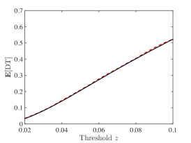
(a) Expected DT

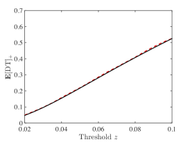
(b) Expected DT conditioned on correct decision

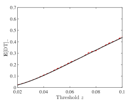
(c) Expected DT conditioned on error

(d) Variance of DT

(e) Variance of DT conditioned on correct decision

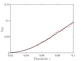
(f) Variance of DT conditioned on error

(g) CV of DT

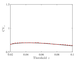
(h) CV of DT conditioned on correct decision

(i) CV of DT conditioned on error

Figure 1: Expected decision times, variances and CVs of decision times for a DDM with $a=0.2$, $\sigma=0.1$, and $x_{0}=-0.01$, showing dependence on threshold $z$. Solid curves represent functions derived in §3 and §4; dashed line segments connect point values obtained by 10,000 Monte-Carlo simulations of Eqn. (1). Note the non-monotonicity evident in panel h.

In Figs. 1 and 2 key expressions derived above are plotted vs. threshold $z$ for the DDM (1) with $a=0.2$, $\sigma=0.1$, and $x_{0}=-0.01$. These parameter values were chosen as representative of fits to human data (e.g. [26]), and to illustrate the general forms of the functions. Drift values in this case might be expected to range from -0.4 to 0.4 (e.g. [22]). See also, among many others, [3, 2, 5, 8], for similar ranges of fitted parameter values. The results of Monte-Carlo simulations of Eqn. (1) using the Euler-Maruyama method [16] with step size $10^{-4}$ are also shown for comparison. Note that, even with 10,000 sample paths, numerical estimates of the third moment and skewness have not converged very well.

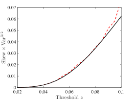
(a) Third central moment of DT

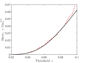
(b) Third central moment of DT conditioned on correct decision

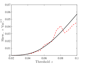
(c) Third central moment of DT conditioned on incorrect decision

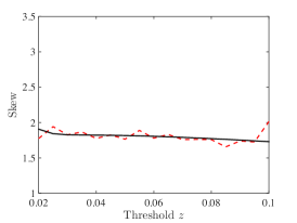
(d) Skewness of DT

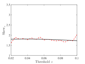
(e) Skewness of DT conditioned on correct decision

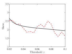
(f) Skewness of DT conditioned on incorrect decision

Figure 2: Third central moments and skewnesses of decision times for a DDM with $a=0.2$, $\sigma=0.1$, and $x_{0}=-0.01$, showing dependence on threshold $z$. Solid curves represent functions derived in §3 and §4; dashed line segments connect point values obtained by 10,000 Monte-Carlo simulations of Eqn. (1).

5 Behavior of CVs

We first consider the unconditional CV with unbiased starting point $x_{0}=k_{x}=0$, for which we can prove the following result.

Proposition 5.1.

Behavior of CVs of decision times for the DDM. The CV for the double-threshold DDM with $k_{x}=0$, Eqn. (14), is bounded above by the CV for the single-threshold DDM, Eqn. (4):

$$\frac{\sqrt{\frac{1}{k_{z}}(1-e^{-4k_{z}}-4k_{z}e^{-2k_{z}})}}{1-e^{-2k_{z}}}\stackrel{{\scriptstyle\rm{def}}}{{=}}F(k_{z})<\sqrt{\frac{1}{k_{z}}}.$$ (39)

Moreover, $F(0)=\sqrt{2/3}$ and $F(k_{z})$ decays monotonically as $k_{z}$ increases.

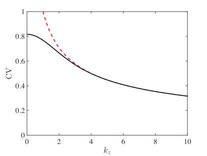
Figure 3: Coefficients of variation as functions of $k_{z}$ for the single threshold DDM (dashed) and the DDM with double thresholds and $k_{x}=0$ (solid).

For the proof of the above proposition see Appendix D. Fig. 3 illustrates the proposition by plotting both CV functions over the range $0\leq k_{z}\leq 10$.

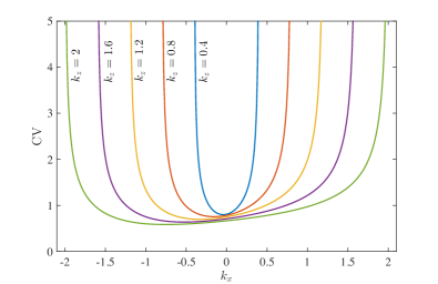
(a) Unconditioned CV vs. $k_{x}$

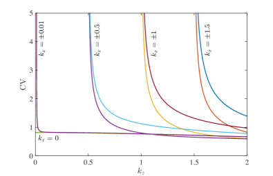
(b) Unconditioned CV vs. $k_{z}$

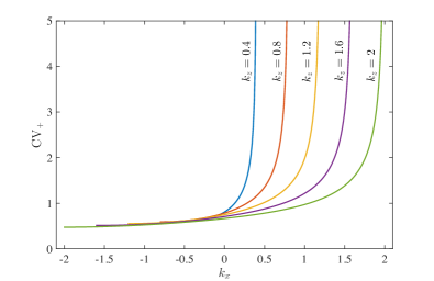
(c) CV conditioned on correct decision vs. $k_{x}$

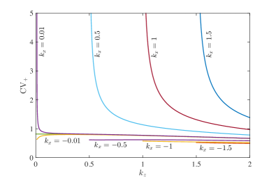
(d) CV conditioned on correct decision vs. $k_{z}$

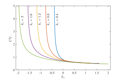
(e) CV conditioned on error vs. $k_{x}$

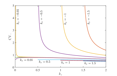
(f) CV conditioned on error vs. $k_{z}$

Figure 4: Coefficients of variation of decision time as functions of $k_{x}=ax_{0}/\sigma^{2}$ for several $k_{z}$’s (left column) and $k_{z}=az/\sigma^{2}$ for several $k_{x}$’s (right column). Unconditioned CVs are shown in top row, conditioned CVs in middle and bottom rows. Observe the symmetry $k_{x}\mapsto-k_{x}$ relating the latter, as noted at the beginning of §4.

It seems difficult to prove a result analogous to Proposition 5.1 for the general CV expressions of Eqns. (10) and (31) due to their complexity. However, plots of the unconditional and conditional CVs as functions of the normalized threshold and starting point $k_{z}=az/\sigma^{2}$ and $k_{x}=ax_{0}/\sigma^{2}$ shown in Fig. 4 illustrate their behavior over the ($k_{z},k_{x}$)-plane.

Here, as shown in Proposition 5.1 and Eqns. (34-35), for $k_{x}=0$ both conditioned and unconditioned CVs converge to $\sqrt{2/3}$ from below as $k_{z}\to 0^{+}$ (see right column). However, for $k_{x}\neq 0$, the behavior is significantly different. In particular, as shown in §3, Eqns. (25-26), the unconditioned CVs diverge as $k_{x}\to\pm k_{z}$ (see left column). CVs for symmetric starting points $\pm k_{x}$ diverge along different curves as $|k_{x}|\to k_{z}$; however, these curves converge to each other as $k_{z}\to 0^{+}$ (see left column). Similarly, CVs conditioned on correct responses and errors diverge as $k_{x}\to k_{z}$ and $k_{x}\to-k_{z}$ respectively. Interestingly, CVs conditioned on correct responses and errors converge to finite limits smaller than $\sqrt{2/3}$ as $k_{x}\to-k_{z}<0$ and $k_{x}\to k_{z}>0$ respectively. In Fig. 4(d), as shown in §4, $\mathrm{CV}_{+}$ converges to $\sqrt{2/5}$ as $k_{x}\to-k_{z}$ and $k_{z}\to 0^{+}$. It is interesting to note that this convergence is not monotone.

The bottom four panels of Fig. 4 illustrate the symmetry of moments conditioned on correct responses and errors with respect to $k_{x}\mapsto-k_{x}$, noted at the beginning of §4. Unlike the case $k_{x}=0$ for which CV is monotonic in $k_{z}$, as shown in Proposition 5.1, conditioned CVs are not monotone functions of $z$ or $k_{z}$ in general. Some instances of non-monotonicity appear in Figs. 1(h), 4(d) and 4(f) above.

6 Behavior of moments for the extended DDM

We end by describing some results for the extended DDM introduced by Ratcliff [20], specifically, the effects of drawing drift rates and starting points for Eqn. (1) from Gaussian and uniform distributions $\mathcal{N}(a,\sigma_{a})$ and $\mathcal{U}(x_{0}-\frac{s_{x}}{2},x_{0}+\frac{s_{x}}{2})$ respectively, where $x_{0}\pm\frac{s_{x}}{2}\in[-z,z]$, and standard deviation $\sigma_{a}$ and range $s_{x}$ characterize trial-to-trial variability of drift rates and starting points. Complete analytical results on moments for this extended model are not known, and we therefore perform numerical studies. In particular we investigate departures from the analytical results derived above as the variance/range of the distributions $\mathcal{N}$ and $\mathcal{U}$ increase from zero. We also consider the effects of non-decision time.

6.1 Analytical and semi-analytical expressions

We first discuss how expressions for the moments of decision times and error rate for the pure DDM can be leveraged to efficiently compute analogous explicit expressions for the extended DDM. For clarity, we denote the decision time of the pure DDM for a given drift rate $a$ and starting point $x_{0}$ by $\tau(a,x_{0})$, and the error rate by ${\rm ER}(a,x_{0})$. The following expressions for the extended DDM are illustrated in Fig. 5.

The error rate of the extended DDM is the expected value of the error rate of the pure DDM averaged over the distributions of drift rates and starting points:

$$\overline{\rm ER}=\mathbb{E}_{A}\big{[}\mathbb{E}_{X_{0}}\big{[}{\rm ER}(A,X_{0})\big{]}\big{]},$$ (40)

where $\mathbb{E}_{Y}[\cdot]$ denotes the expected value computed over the distribution of random variable $Y$. The expectation over the random starting point $X_{0}$ in (40) can be computed explicitly as

$$\mathbb{E}_{X_{0}}[{\rm ER}(a,X_{0})]=\frac{e^{-2k_{x}}\operatorname{sinch}(2k_{\delta})-e^{-2k_{z}}}{e^{2k_{z}}-e^{-2k_{z}}},$$ (41)

where $k_{\delta}=a\delta/\sigma^{2}$ and $\operatorname{sinch}(\cdot):=\sinh(\cdot)/(\cdot)$. Note that this expression reduces to Eqn. (6) for $\delta=0$, using $\operatorname{sinch}(0)=1$.

The non-central moments of the decision times can be computed similarly. In particular, if $T_{n}(a,x_{0})$ is the non-central $n$-th moment of the decision time for the pure DDM, then the non-central $n$-th moment for the extended DDM is

$$\bar{T}_{n}=\mathbb{E}_{A}\big{[}\mathbb{E}_{X_{0}}\big{[}T_{n}(A,X_{0})\big{]}\big{]}.$$ (42)

The non-central moments obtained using Eqn. (42) can be used with Eqns. (10) and (21) to compute variance and skewness of decision time for the extended DDM. Eqn. (42) is valid for both unconditional and conditional moments. The above expressions for the error rate and expected decision time for the extended DDM can be found in [4, Appendix, pp 761–763].

For unconditional moments, the expectation over $X_{0}$ in (42) can be computed in closed form for first two moments, which may be written as

$$\mathbb{E}_{X_{0}}[T_{1}(a,X_{0})] =\frac{\sigma^{2}}{a^{2}}\left(k_{z}\coth(2k_{z})-k_{z}e^{-2k_{x}}\operatorname{sinch}(2k_{\delta})\operatorname{csch}(2k_{z})-k_{x}\right);$$ (43)

$$\mathbb{E}_{X_{0}}[T_{2}(a,X_{0})] =\frac{\sigma^{4}}{a^{4}}\Big{(}k_{z}^{2}+4k_{z}^{2}\operatorname{csch}^{2}(2k_{z})+k_{z}\coth(2k_{z})-4k_{z}^{2}e^{-2kx_{0}}\operatorname{sinch}(2k_{\delta})\operatorname{csch}(2k_{z})\coth(2k_{z})$$

$$-k_{z}e^{-2kx_{0}}\operatorname{sinch}(2k_{\delta})\operatorname{csch}(2k_{z})-k_{x}+k_{x}^{2}+\frac{k_{\delta}^{2}}{3}-2k_{z}k_{x}\coth(2k_{z})$$

$$-2k_{z}k_{x}e^{-2k_{x}}\Big{(}\operatorname{sinch}(2k_{\delta})+\frac{\operatorname{sinch}(2k_{\delta})-\cosh(2k_{d})}{2k_{x}}\Big{)}\operatorname{csch}(2k_{z})\Big{)}.$$ (44)

Expected values in Eqn. (42), involving integrals over the Gaussian distribution that are not tractable in closed form, can easily be computed numerically, for example, using Simpson’s rule.

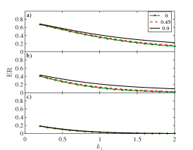
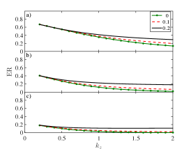
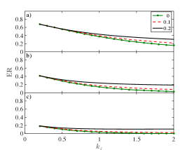
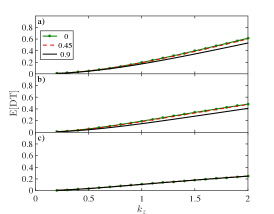
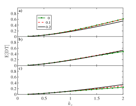
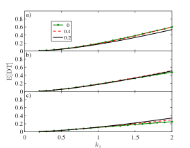
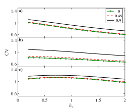
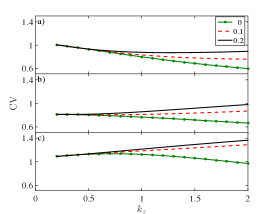
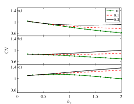
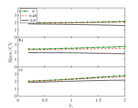
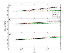
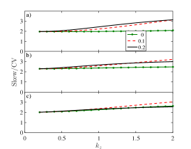
Figure 5: Behavior of moments for the extended DDM. In all panels $a=0.2$ and $\sigma=0.1$. Three sub-panels in each panel correspond to $x_{0}=-z/2,0$ and $z/2$, respectively, from top to bottom. Left panels correspond to $\sigma_{a}=0$ and green solid with dots, red dashed, and black solid curves to $\frac{s_{x}}{2}=0,0.45\min\{z-x_{0},x_{0}+z\}$ and $0.9\min\{z-x_{0},x_{0}+z\}$, respectively. Middle panels correspond to $s_{x}=0$ and green solid with dots, red dashed, and black solid curves to $\sigma_{a}=0,0.1$ and $0.2$, respectively. Right panels are analogous to middle panels and correspond to $\frac{s_{x}}{2}=0.45\min\{z-x_{0},x_{0}+z\}$.

Fig. 5 illustrates the behavior of the unconditional moments of the extended DDM, computed as described above. The introduction of variability in starting points results in increase in error rate, decrease in expected decision time, increase in CV, and decrease in skewness to CV ratio. Introduction of variability in drift rate also causes increase in error rate, decrease in expected decision time and increase in CV, but the skewness to CV ratio increases (compare bottom panels). Interestingly, for high values of drift rate variability CV is a monotonically increasing function of $k_{z}$, in contrast to the behavior of CV for pure DDM discussed in §5. The effect of drift rate variability seems to dominate when both initial condition and drift rate variability are present.

6.2 Effect of non-decision time

Before returning to the extended DDM, we investigate the role of the non-decision part of the reaction time, the sensory-motor latency, on its $\rm CV$ and skewness. Recall that $\rm RT=\rm DT+\rm T_{\textup{nd}}$, where $\rm T_{\textup{nd}}$ is the non-decision time. We define the following coefficients to characterize the dependence of $\rm DT$ and $\rm T_{\textup{nd}}$:

$$\rho_{11} =\frac{\mathbb{E}[(\rm DT-\mathbb{E}[\rm DT])(\rm T_{\textup{nd}}-\mathbb{E}[\rm T_{\textup{nd}}])]}{\sqrt{\rm Var[\rm DT]\;Var[\rm T_{\textup{nd}}]}},$$ (45)

$$\rho_{12} =\frac{\mathbb{E}[(\rm DT-\mathbb{E}[\rm DT])(\rm T_{\textup{nd}}-\mathbb{E}[\rm T_{\textup{nd}}])^{2}]}{\sqrt{\rm Var[\rm DT]\;\mathbb{E}[(\rm T_{\textup{nd}}-\mathbb{E}[\rm T_{\textup{nd}}])^{4}]}},$$ (46)

$$\rho_{21} =\frac{\mathbb{E}[(\rm DT-\mathbb{E}[\rm DT])^{2}(\rm T_{\textup{nd}}-\mathbb{E}[\rm T_{\textup{nd}}])]}{\sqrt{\mathbb{E}[(\rm DT-\mathbb{E}[\rm DT])^{4}\;Var[\rm T_{\textup{nd}}]}}.$$ (47)

Note that $\rho_{11}$ is the standard correlation coefficient between $\rm DT$ and $\rm T_{\textup{nd}}$, and $\rho_{12}$, $\rho_{21}$ can be interpreted as higher order correlation coefficients. If $\rm DT$ and $\rm T_{\textup{nd}}$ are independent, then all these correlation coefficients are zero. In this case, it follows from the definition of RT that

$$\mathbb{E}[\rm RT] =\mathbb{E}[\rm DT]+\mathbb{E}[\rm T_{\textup{nd}}]$$

$${\rm Var}[\rm RT] ={\rm Var}[\rm DT]+{\rm Var}[\rm T_{\textup{nd}}]+2\rho_{11}\sqrt{{\rm Var}[\rm DT]\;{\rm Var}[\rm T_{\textup{nd}}]}$$

$$\mathbb{E}[({\rm RT}-\mathbb{E}[{\rm RT}])^{3}] ={\rm Skew}[\rm DT]{\rm Var}[\rm DT]^{3/2}+{\rm Skew}[\rm T_{\textup{nd}}]{\rm Var}[\rm T_{\textup{nd}}]^{3/2}$$

$$+3\rho_{12}\sqrt{{\rm Kur}[T_{\textup{nd}}]{\rm Var}[\rm DT]}{\rm Var}[\rm T_{\textup{nd}}]+3\rho_{21}\sqrt{{\rm Kur}[\rm DT]{\rm Var}[\rm T_{\textup{nd}}]}{\rm Var}[\rm DT],$$

where $\rm Kur[\cdot]$ is the kurtosis. The conditional mean decision time and variance can be defined similarly by introducing conditional equivalents of correlation coefficients (45-47). However, for simplicity of exposition, in the following we assume that non-decision time and decision time are independent; accordingly, the above correlation coefficients are zero. Formulae for $\rm CV$ and $\rm Skew$ for $\rm RT$’s follow immediately from above expressions. For use below, we assume $\rm T_{\textup{nd}}$ is uniformly distributed with mean $\mathbb{E}[\rm T_{\textup{nd}}]$ and range $s_{t}$.

6.3 Effects of trial-to-trial variability

Seeking to provide a more complete picture, we conducted simulations of the extended and pure DD models. To obtain the following simulation results we used the RTdist package for graphical processing unit (GPU) based simulation of the DDM [31] to simulate a large subset of the parameter space spanning the range of plausible parameter values. We simulated $1,518,750$ parameter combinations in about $5.5$ hours on a Tesla NVIDIA GPU, with $1$ msec timesteps up to 5 secs maximum RT, with $10^{5}$ trials simulated per parameter combination. In Fig. 6, the noise level was fixed at $\sigma=0.1$ and we varied mean drift $a$ and threshold $z$ over the ranges $[0.1,1.0]$ and $[0.05,0.3]$ respectively. Fig. 6 shows accuracy, mean RT, CV, skewness to CV ratio (SCV) and the percentage of trials that failed to cross threshold within 5 secs. (The latter quantity is small except for low drift and high threshold, where it rises to $15-20\%$.) Note that the left hand column of Fig. 6 show results for the pure DDM with $\rm T_{\textup{nd}}=0$, and thus provide standards for comparison with other cases. See Appendix E for additional simulation results.

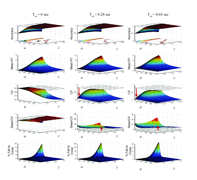
Figure 6: Effect of deterministic non-decision time $\rm T_{\textup{nd}}$ in the extended DDM. Left column: $\rm T_{\textup{nd}}=0$ sec. Middle column: $\rm T_{\textup{nd}}=0.28$ sec. Right column: $\rm T_{\textup{nd}}=0.45$ sec. Curves plotted on the drift-threshold plane in top row denote equally spaced contours of the accuracy surface; red arrows show the effect of increasing $\rm T_{\textup{nd}}$ on CV and SCV.

The most profound effect on higher moments of the RT distributions is due to changes in non-decision latency, $\rm T_{\textup{nd}}$, as shown in Fig. 6. Specifically, note the dramatic drop in the CV of RTs as $\rm T_{\textup{nd}}$ increases from 0 to $0.28$ sec, and the corresponding increase of skewness to CV ratio (red arrows, row 3).

Fig. 7 shows this phenomenon most clearly, using behaviorally plausible values for the extended DDM. When the correct expected non-decision latency of $0.45$ sec is subtracted from the RTs, the CV (middle plot) approaches $\sqrt{2/3}\approx 0.8165$ as drift approaches 0. Thus researchers may be able to estimate $\rm T_{\textup{nd}}$ at low accuracy levels when behavior is unbiased toward either alternative by progressively subtracting from the RT until the CV approaches $\sqrt{2/3}$ from below (cf. Proposition 5.1 and Fig. 3). In contrast, the SCV ratio grows substantially as drift, and hence accuracy, increase (Fig. 6, red arrows, row 4). Researchers may therefore be able to estimate $\rm T_{\textup{nd}}$ at high drift levels by subtracting postulated non-decision time from the RT until the SCV ratio declines to 3. These two heuristics for estimating $\rm T_{\textup{nd}}$ independently at both low and high levels of drift may provide robust and easily-computable sanity checks for constraining the values of $\rm T_{\textup{nd}}$ when using fitting algorithms.

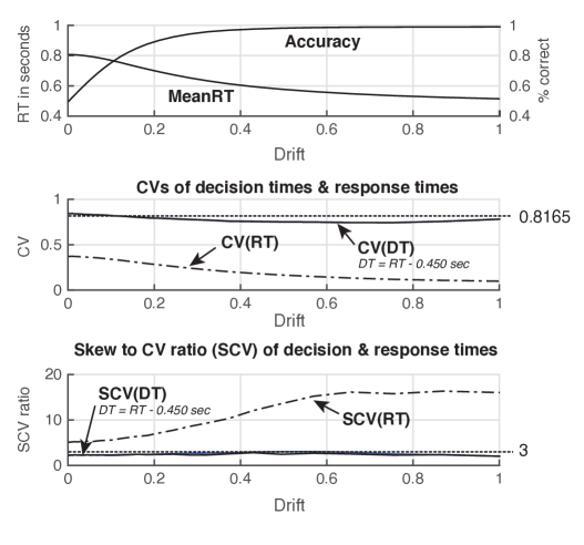
Figure 7: Comparison of CVs and SCVs, as a function of drift, computed from raw RTs (dot-dashed) and from DTs (solid). DTs have the true, average non-decision latency of $0.45$ sec subtracted. Representative levels of extended DDM parameter values were used ($z=0.06$, $x_{0}=0$, $\delta=0.5\cdot z$ , $\sigma_{a}=0.25\cdot a$, $\mathbb{E}[\rm T_{\textup{nd}}]=0.45$ sec, and $s_{t}=0.112$ sec.)

7 Conclusion

We analyzed in detail the first three moments of decision times of the pure and extended DDMs. We derived explicit expressions for unconditional and conditional moments and used these expressions to thoroughly investigate the behavior of the CV and skewness of decision times in terms of two useful parameters: the non-dimensional threshold and non-dimensional initial condition ($k_{z}$ and $k_{x}$, Eqn. (2)). These expressions are summarized in Table 1. The MatLab and R code for these expressions is available at: https://github.com/PrincetonUniversity/higher_moments_ddm.

In particular, we computed several limits of interest for the pure DDM. We established that, for an unbiased starting point ($x_{0}=0$), the CV of decision times is a monotonically decreasing function of $k_{z}$ and that it approaches $\sqrt{2/3}$ as $k_{z}\rightarrow 0$ (Proposition 5.1 and Fig. 3). In the limits of small drift rate and unbiased starting point, we showed that the ratio of skewness to CV approaches $12/5$. Furthermore, for non-zero drift rates and in the limit of large thresholds (high accuracy), we showed that skewness to CV ratio approaches $3$. We showed that both CV and skewness of decision times diverge as the starting point approaches either threshold; however, the ratio of skewness to CV is a bounded function of non-dimensional threshold. We also showed that in the limit of large thresholds, these moments match those of first passage times for single-threshold drift-diffusion processes, and we established similar results for conditional CV and skewness of decision times. We established that the decision time distribution for the double-threshold DDM converges to he decision time distribution of the single-threshold DDM for large thresholds (Appendix C).

	1-threshold	2-threshold
Error rate
ER	NA	$\frac{e^{-2k_{x}}-e^{-2k_{z}}}{e^{2k_{z}}-e^{-2k_{z}}}$
Mean
$\rm\mathbb{E}[DT]$	$\frac{\sigma^{2}}{a^{2}}(k_{z}-k_{x})$	$\frac{\sigma^{2}}{a^{2}}\left[k_{z}\coth(2k_{z})-k_{z}e^{-2k_{x}}\operatorname{csch}(2k_{z})-k_{x}\right]$
$\rm\mathbb{E}[DT]_{+}$	NA	$\frac{\sigma^{2}}{a^{2}}\left(2k_{z}\coth(2k_{z})-(k_{x}+k_{z})\coth(k_{x}+k_{z})\right)$
Variance
$\rm Var$	$\frac{\sigma^{4}}{a^{4}}(k_{z}-k_{x})$	see equation (10)
$\rm Var_{+}$	NA	see equation (31)
Coefficient of Variation
$\rm CV$	$\frac{1}{\sqrt{k_{z}-k_{x}}}$	see equation (13)
$\rm CV_{+}$	NA	see equation (33)
Skewness
$\rm Skew\times Var^{3/2}$	$\frac{3\sigma^{6}}{a^{6}}(k_{z}-k_{x})$	see equation (21)
$\rm Skew_{+}\times Var_{+}^{3/2}$	NA	see equation (36)

Table 1: Summary of expressions of error rate and moments of decision time.

We then derived analytic and semi-analytic expressions for the moments of decision times of the extended DDM, and numerically investigated the effects of trial-to-trial variability in starting points and drift rates on the DDM’s performance. We observed that variability in drift rate appears to dominate these effects, compared to starting point variability.

Finally, we investigated the effect of non-decision times (sensory-motor latencies, $\rm T_{\textup{nd}}$) on decision-making performance. We observed that CVs of reaction times (${\rm DT}+\rm T_{\textup{nd}}$) decrease and their skewness-to-CV ratios increase as mean $\rm T_{\textup{nd}}$’s increase (Fig. 6). We propose that the decrease in CVs and increase in skewness-to-CV ratios could be used to estimate non-decision times in low and high accuracy regimes respectively (see Fig. 7). The development of rigorous methods using these metrics to estimate non-decision time is a potential avenue for future research.

It should be noted that difficulties in estimating higher moments of empirical RT data have been highlighted in the literature [18, 21]. However, at least in the context of interval-timing tasks, predictions regarding CV and skewness have proved to be useful in discriminating between different models [25, 28]. Furthermore, it is possible that future two-alternative perceptual decision task designs could be found that would yield data amenable to estimation of higher moments, in which case, the expressions we derive here may prove helpful.

More generally, the explicit expressions derived in this paper can be used to quickly identify ranges of parameters that are relevant to fitting specific behavioral data sets, thereby reducing the volumes of multi-dimensional space in which parameter fits need to be run. In principle, the cumulant generating function method outlined in Appendix A can be used to produce formulae for fourth and higher moments, and although the results will be complex, they and their limiting behaviors may also provide guidance for parameter fitting.

Appendices

Appendix A Error rate and unconditional variance of decision time

In this section we show that error rate (6) and expected decision time (7) are equivalent to the expressions given in the subsection “The Drift Diffusion Model” of [4, Appendix, Eqns. (A27-31)]. In our notation, the quantities $\tilde{z}$ and $\tilde{a}$ defined in [4] are

$$\tilde{z}=\frac{z}{a},\quad\text{and}\quad\tilde{a}=\frac{a^{2}}{\sigma^{2}}.$$

Define $\tilde{x}_{0}=x_{0}/a$. Note that $k_{z}=\tilde{z}\tilde{a}$ and $k_{x}=\tilde{a}\tilde{x}_{0}$. Also note that $\tilde{x}_{0}$ and $x_{0}$ are referred to as $x_{0}$ and $y_{0}$, respectively in [4].

The expression (6) for error rate may be rewritten as follows

$$\mathrm{ER}=\frac{e^{-2k_{x}}-e^{-2k_{z}}}{e^{2k_{z}}-e^{-2k_{z}}}=\frac{1-e^{-2k_{z}}}{e^{2k_{z}}-e^{-2k_{z}}}-\frac{1-e^{-2k_{x}}}{e^{2k_{z}}-e^{-2k_{z}}} =\frac{e^{2k_{z}}-1}{e^{4k_{z}}-1}-\frac{1-e^{-2k_{x}}}{e^{2k_{z}}-e^{-2k_{z}}}$$

$$=\frac{e^{2k_{z}}-1}{(e^{2k_{z}}+1)(e^{2k_{z}}-1)}-\frac{1-e^{-2k_{x}}}{e^{2k_{z}}-e^{-2k_{z}}} =\frac{1}{1+e^{2k_{z}}}-\frac{1-e^{-2k_{x}}}{e^{2k_{z}}-e^{-2k_{z}}}$$

$$=\frac{1}{1+e^{2\tilde{z}\tilde{a}}}-\left[\frac{1-e^{-2\tilde{x}_{0}\tilde{a}}}{e^{2\tilde{z}\tilde{a}}-e^{-2\tilde{z}\tilde{a}}}\right],$$ (48)

which is identical to the ER expression in [4]. Similarly,

$$\mathbb{E}[{\rm DT}] =\frac{\sigma^{2}}{a^{2}}\left[k_{z}\coth(2k_{z})-k_{z}e^{-2k_{x}}\operatorname{csch}(2k_{z})-k_{x}\right]$$

$$=\frac{\sigma^{2}}{a^{2}}k_{z}\left[\coth(2k_{z})-\operatorname{csch}(2k_{z})+(1-e^{-2k_{x}})\operatorname{csch}(2k_{z})-\frac{k_{x}}{k_{z}}\right]$$

$$=\frac{z}{a}\left[\frac{e^{2k_{z}}+e^{-2k_{z}}-2}{e^{2k_{z}}-e^{-2k_{z}}}+(1-e^{-2k_{x}})\operatorname{csch}(2k_{z})-\frac{x_{0}}{z}\right]$$

$$=\frac{z}{a}\tanh(k_{z})+\frac{2z}{a}\frac{(1-e^{-2k_{x}})}{e^{2k_{z}}-e^{-2k_{z}}}-\frac{x_{0}}{a}$$

$$=\tilde{z}\tanh(\tilde{z}\tilde{a})+\frac{2\tilde{z}(1-e^{-2\tilde{a}\tilde{x}_{0}})}{e^{2\tilde{a}\tilde{z}}-e^{-2\tilde{z}\tilde{a}}}-\tilde{x}_{0},$$ (49)

which is identical to the expected decision time expression in [4].

Appendix B Unconditional variance of decision time

The second moment of the decision time $T_{2}$ is the solution of the following linear ODE:

$$a\frac{dT_{2}}{dx_{0}}+\frac{\sigma^{2}}{2}\frac{d^{2}T_{2}}{dx^{2}_{0}}=-2\mathbb{E}[{\rm DT}],$$ (50)

with boundary conditions $T_{2}(\pm z)=0$ (e.g. [10, §5.5.1; see Eqn. (5.5.19) for the general $n$’th moment ODE]). To solve Eqn. (50) we first rewrite $\mathbb{E}[{\rm DT}]$ to make dependence on the starting point $x_{0}$ explicit:

$$\mathbb{E}[{\rm DT}]=\alpha_{1}-\alpha_{2}e^{-2kx_{0}}-\frac{x_{0}}{a}.$$

Here $\alpha_{1}=\frac{z}{a}\coth(2k_{z})$, $\alpha_{2}=\frac{z}{a}\operatorname{csch}(2k_{z})$ and unlike $k_{z},k_{x}$ defined above, $k=\frac{a}{\sigma^{2}}$ is independent of $z$ and $x_{0}$. A particular solution to (50) is

$$T_{2}^{p}=\frac{x_{0}^{2}}{a^{2}}-\alpha_{3}x_{0}-\frac{2\alpha_{2}}{a}x_{0}e^{-2kx_{0}},$$

where $\alpha_{3}=\frac{2}{a}(\alpha_{1}+\frac{1}{2ka})$, and the general solution takes the form

$$T_{2}(x_{0})=c_{1}+c_{2}e^{-2kx_{0}}+\frac{x_{0}^{2}}{a^{2}}-\alpha_{3}x_{0}-\frac{2\alpha_{2}}{a}x_{0}e^{-2kx_{0}}.$$

Substituting the boundary conditions $T_{2}(\pm z)=0$, and solving for $c_{1}$ and $c_{2}$, we obtain

$$c_{1} =\frac{2z^{2}}{a^{2}}\coth^{2}(2k_{z})+\frac{z}{ka^{2}}\coth(2k_{z})-\frac{z^{2}}{a^{2}}+\frac{2z^{2}}{a^{2}}\operatorname{csch}^{2}(2k_{z})$$

$$=\frac{z^{2}}{a^{2}}+\frac{4z^{2}}{a^{2}}\operatorname{csch}^{2}(2k_{z})+\frac{z}{ka^{2}}\coth(2k_{z}),\quad\text{and }$$

$$c_{2} =-\frac{4z^{2}}{a^{2}}\operatorname{csch}(2k_{z})\coth(2k_{z})-\frac{z}{ka^{2}}\operatorname{csch}(2k_{z}),$$

and we therefore find that

$$T_{2}=\frac{z^{2}}{a^{2}}+\frac{4z^{2}}{a^{2}}\operatorname{csch}^{2}(2k_{z}) +\frac{\sigma^{2}z}{a^{3}}\coth(2k_{z})-\frac{4z^{2}e^{-2kx_{0}}}{a^{2}}\operatorname{csch}(2k_{z})\coth(2k_{z})-\frac{\sigma^{2}ze^{-2kx_{0}}}{a^{3}}\operatorname{csch}(2k_{z})$$

$$+\frac{x_{0}^{2}}{a^{2}}-\frac{2zx_{0}}{a^{2}}\coth(2k_{z})-\frac{\sigma^{2}x_{0}}{a^{3}}-\frac{2zx_{0}e^{-2kx_{0}}}{a^{2}}\operatorname{csch}(2k_{z}).$$ (51)

We can now obtain the expression for the variance of decision time:

$$\mathrm{Var} =T_{2}-\mathbb{E}[{\rm DT}]^{2}$$

$$=\frac{3z^{2}}{a^{2}}\operatorname{csch}^{2}(2k_{z})+\frac{\sigma^{2}z}{a^{3}}\coth(2k_{z})-\frac{\sigma^{2}x_{0}}{a^{3}}-\frac{2z^{2}e^{-2kx_{0}}}{a^{2}}\operatorname{csch}(2k_{z})\coth(2k_{z})$$

$$-\frac{\sigma^{2}ze^{-2kx_{0}}}{a^{3}}\operatorname{csch}(2k_{z})-\frac{4zx_{0}e^{-2kx_{0}}}{a^{2}}\operatorname{csch}(2k_{z})-\frac{z^{2}e^{-4kx_{0}}}{a^{2}}\operatorname{csch}^{2}(2k_{z}).$$ (52)

Equivalently, we may write

$$\mathrm{Var} =\frac{\sigma^{4}}{a^{4}}\left[3k_{z}^{2}\operatorname{csch}^{2}(2k_{z})-2k_{z}^{2}e^{-2k_{x}}\operatorname{csch}(2k_{z})\coth(2k_{z})-4k_{z}k_{x}e^{-2k_{x}}\operatorname{csch}(2k_{z})\right.$$

$$\left.-k_{z}^{2}e^{-4k_{x}}\operatorname{csch}^{2}(2k_{z})+k_{z}\coth(2k_{z})-k_{z}e^{-2k_{x}}\operatorname{csch}(2k_{z})-k_{x}\right].$$ (53)

Appendix C Method for computation of conditional moments

The moment generating function $M_{X}:\mathcal{H}\rightarrow\mathbb{R}_{>0}$ of a random variable $X$ is defined by

$$M_{X}(\alpha):=\mathbb{E}[e^{\alpha X}],$$

provided the expectation exists for each $\alpha$ in some neighborhood of zero, i.e., for each $\alpha\in\mathcal{H}$, where $\mathcal{H}\subset\mathbb{R}$ is some interval containing zero. The moment generating function is a special case of the characteristic function defined on the complex plane (see [14, §5.7, Theorem 12]), and from it the cumulant generating function $K_{X}:\mathcal{H}\rightarrow\mathbb{R}$ of $X$ can be obtained by taking the natural logarithm:

$$K_{X}(\alpha)=\log M_{X}(\alpha).$$ (54)

The $n$-th cumulant $\kappa_{n}$ of $X$ is defined as $\kappa_{n}=\frac{d^{n}K_{X}(\alpha)}{d\alpha^{n}}\big{|}_{\alpha=0}$, or equivalently $K_{X}(\alpha)=\sum_{n=1}^{\infty}\frac{\kappa_{n}\alpha^{n}}{n!}$. It can then be shown that

$$\kappa_{1}=\mu_{1},\quad\kappa_{2}=\mu^{\textup{cen}}_{2},\quad\kappa_{3}=\mu^{\textup{cen}}_{3},\quad\text{and }\kappa_{4}=\mu^{\textup{cen}}_{4}-3\kappa_{2}^{2},$$

where $\mu_{n}=\mathbb{E}[X^{n}]$ and $\mu^{\textup{cen}}_{n}=\mathbb{E}[(X-\mathbb{E}[X])^{n}]$ denote the $n$th non-central and central moments. Thus, successive moments of the distribution from which $X$ is drawn can be generated from $M_{X}(\alpha)$. For further details and derivations of moment generating functions, see [15, Chap 4, §6] and [10, §2.6].

We now derive the moment generating function for DTs of the DDM (1). We define $M_{\textup{DT}}:\mathcal{A}\rightarrow\mathbb{R}_{>0}$, $M_{+}:\mathcal{A}\rightarrow\mathbb{R}_{>0}$, and $M_{-}:\mathcal{A}\rightarrow\mathbb{R}_{>0}$ by

$$M_{\textup{DT}}(\alpha)=\mathbb{E}[e^{\alpha\tau}],\quad M_{+}(\alpha)=\mathbb{E}[e^{\alpha\tau}|x(\tau)=z],\quad\text{and }M_{-}(\alpha)=\mathbb{E}[e^{\alpha\tau}|x(\tau)=-z],$$ (55)

where $\mathcal{A}\subset\mathbb{R}$ is some interval containing zero in which the above expectations exist. $M_{\textup{DT}}(\alpha)$, $M_{+}(\alpha)$ and $M_{-}(\alpha)$ are, respectively, the moment generating functions for unconditional decision times (for all responses) and for decision times conditioned on correct responses and on errors. Expressions for these functions are well known in the literature (e.g. [6]). Here, for completeness, we derive them from first principles.

We begin by deriving an expression for $M_{+}(\alpha)$. We note that for a given set of parameters $a,\sigma,z$, and $\alpha$, $M_{+}(\alpha)$ depends only on $x_{0}$. Let $\tau(x_{0})$ denote the decision time (DT) starting from initial condition $x_{0}$. Define $g:\mathbb{R}\rightarrow\mathbb{R}_{>0}$ as the map from initial condition $x_{0}$ to $M_{+}(\alpha)\mathbb{P}(x(\tau)=z)$, i.e.,

$$g(x_{0})=\mathbb{E}[e^{\alpha\tau(x_{0})}\boldsymbol{1}(x(\tau(x_{0}))=z)],$$ (56)

where $\boldsymbol{1}(\cdot)$ is the indicator function.

Consider the evolution of the DDM (1) starting from $x_{0}$ at $t=0$ for an infinitesimal duration $h\in\mathbb{R}_{>0}$. Let $X_{h}:=x(h)=x_{0}+ah+\sigma W(h)$. It follows that

$$g(x_{0}) =\mathbb{E}_{X_{h}}\mathbb{E}_{\tau(X_{h})}[e^{\alpha(h+\tau(X_{h}))}]$$

$$=e^{\alpha h}\mathbb{E}_{X_{h}}[g(X_{h})]$$

$$=e^{\alpha h}\Big{(}g(x_{0})+\frac{dg}{dx_{0}}ah+\frac{1}{2}\frac{d^{2}g}{dx_{0}^{2}}\sigma^{2}h\Big{)}+O(h^{2}),$$

where $O(h^{2})$ represents terms of order $h^{2}$ and higher. Rearranging terms and setting $h\to 0^{+}$, we obtain the following ODE for $g$

$$\frac{\sigma^{2}}{2}\frac{d^{2}g}{dx_{0}^{2}}+a\frac{dg}{dx_{0}}+\alpha g=0,$$ (57)

with boundary conditions $g(z)=1$ and $g(-z)=0$. The solution to (57) is of the form $g(x_{0})=\zeta_{1}e^{\lambda_{1}x_{0}}+\zeta_{2}e^{\lambda_{2}x_{0}}$, where $\lambda_{1}$ and $\lambda_{2}$ are roots of the equation $\sigma^{2}\lambda^{2}/2+a\lambda+\alpha=0$, i.e.,

$$\lambda_{1}=\frac{-a-\sqrt{a^{2}-2\alpha\sigma^{2}}}{\sigma^{2}},\quad\text{and}\quad\lambda_{2}=\frac{-a+\sqrt{a^{2}-2\alpha\sigma^{2}}}{\sigma^{2}}.$$

Substituting the boundary conditions, we get two simultaneous equations

$$\zeta_{1}e^{\lambda_{1}z}+\zeta_{2}e^{\lambda_{2}z}=1,\quad\text{and }\quad\zeta_{1}e^{-\lambda_{1}z}+\zeta_{2}e^{-\lambda_{2}z}=0,$$

the solution to which is

$$\zeta_{1}=\frac{e^{\lambda_{1}z}}{e^{2\lambda_{1}z}-e^{2\lambda_{2}z}},\quad\text{and}\quad\zeta_{2}=-\frac{e^{\lambda_{2}z}}{e^{2\lambda_{1}z}-e^{2\lambda_{2}z}},$$

and consequently,

$$g(x_{0})=\frac{e^{\lambda_{1}(z+x_{0})}-e^{\lambda_{2}(z+x_{0})}}{e^{2\lambda_{1}z}-e^{2\lambda_{2}z}}=\frac{e^{-a(z+x_{0})/\sigma^{2}}}{e^{-2az/\sigma^{2}}}\frac{\sinh(\frac{(z+x_{0})\sqrt{a^{2}-2\alpha\sigma^{2}}}{\sigma^{2}}}{\sinh(\frac{2z\sqrt{a^{2}-2\alpha\sigma^{2}}}{\sigma^{2}})}=e^{\frac{a(z-x_{0})}{\sigma^{2}}}\frac{\sinh(\frac{(z+x_{0})\sqrt{a^{2}-2\alpha\sigma^{2}}}{\sigma^{2}})}{\sinh(\frac{2z\sqrt{a^{2}-2\alpha\sigma^{2}}}{\sigma^{2}})}.$$

Thus, recalling the definition (56) of $g(x_{0})$, the moment-generating function conditioned on correct decisions is

$$M_{+}(\alpha)=\mathbb{E}[e^{\alpha\tau}|x(\tau)=z]=\frac{e^{\frac{a(z-x_{0})}{\sigma^{2}}}}{\mathbb{P}(x(\tau)=z)}\frac{\sinh(\frac{(z+x_{0})\sqrt{a^{2}-2\alpha\sigma^{2}}}{\sigma^{2}})}{\sinh(\frac{2z\sqrt{a^{2}-2\alpha\sigma^{2}}}{\sigma^{2}})},$$ (58)

and substituting this in the definition (54) yields the cumulant generating function (28) used in §4.

Similarly, we may obtain analogous expressions for incorrect decisions

$$M_{-}(\alpha)=\mathbb{E}[e^{\alpha\tau}|x(\tau)=-z]=\frac{e^{\frac{-a(z+x_{0})}{\sigma^{2}}}}{\mathbb{P}(x(\tau)=-z)}\frac{\sinh(\frac{(z-x_{0})\sqrt{a^{2}-2\alpha\sigma^{2}}}{\sigma^{2}})}{\sinh(\frac{2z\sqrt{a^{2}-2\alpha\sigma^{2}}}{\sigma^{2}})},$$ (59)

and for all decisions, correct and incorrect:

$$M_{\textup{DT}}(\alpha)=\mathbb{E}[e^{\alpha\tau}]=e^{\frac{-a(z+x_{0})}{\sigma^{2}}}\frac{\sinh(\frac{(z-x_{0})\sqrt{a^{2}-2\alpha\sigma^{2}}}{\sigma^{2}})}{\sinh(\frac{2z\sqrt{a^{2}-2\alpha\sigma^{2}}}{\sigma^{2}})}+e^{\frac{a(z-x_{0})}{\sigma^{2}}}\frac{\sinh(\frac{(z+x_{0})\sqrt{a^{2}-2\alpha\sigma^{2}}}{\sigma^{2}})}{\sinh(\frac{2z\sqrt{a^{2}-2\alpha\sigma^{2}}}{\sigma^{2}})}.$$ (60)

It should be noted that in the limit $z\to\infty$

$$M_{\textup{DT}}(\alpha)=\exp\left(\frac{az}{\sigma^{2}}\left(1-\sqrt{1-\frac{2\alpha\sigma^{2}}{a^{2}}}\right)\right),$$

which is the moment generating function of the Wald distribution [6, Eq. 2.0.1], i.e., the decision time distribution of the single-threshold DDM. Consequently, the decision time distribution of the double-threshold DDM converges to the the decision time distribution of the single-threshold DDM as $z\to\infty$.

Appendix D Proof of Proposition 5.1

We first show that the CV for the single-threshold DDM provides an upper bound for the double threshold case. Canceling the $\sqrt{1/k_{z}}$ terms in the inequality (39), squaring, rearranging and dividing by $2e^{-2k_{z}}$ shows that this is equivalent to

$$(1-e^{-2k_{z}})^{2}>(1-e^{-4k_{z}}-4k_{z}e^{-2k_{z}})\Leftrightarrow e^{-2k_{z}}>1-2k_{z},$$ (61)

which clearly holds for all $k_{z}\neq 0$.

We next evaluate the limit of $F(k_{z})$ as $k_{z}\to 0$ by expanding the numerator of Eqn. (39) in Taylor series:

$$\sqrt{\frac{1}{k_{z}}\left[1-\left(1-4k_{z}+\frac{16k_{z}^{2}}{2}-\frac{64k_{z}^{3}}{3!}\right)-\left(4k_{z}(1-2k_{z}+\frac{4k_{z}^{2}}{2})\right)+\mathcal{O}(k_{z}^{4})\right]}=\sqrt{\frac{8}{3}k_{z}^{2}+\mathcal{O}(k_{z}^{3})}.$$

Expanding the denominator likewise, we have

$$F(k_{z})=\frac{\sqrt{\frac{8}{3}k_{z}^{2}+\mathcal{O}(k_{z}^{3})}}{[1-(1-2k_{z}+\mathcal{O}(k_{z}^{2}))]}\to\sqrt{\frac{2}{3}}\mbox{ as }k_{z}\to 0.$$ (62)

The exponentials in the numerator and denominator of $F(k_{z})$ decay rapidly, so that it differs from $\sqrt{1/k_{z}}$ by less than $0.24\%$ for $k_{z}\geq 4$, implying that the slow monotonic decay $\sim k_{z}^{\frac{1}{2}}$ dominates for large $k_{z}$; see Fig. 3. However, the behavior for smaller $k_{z}$ is more subtle and requires computation of all terms in the Taylor series.

To prove monotonic decay throughout we use the fact that $F(k_{z})>0$ and show that the derivative of

$$F^{2}(k_{z})=\frac{\left(\frac{1-e^{-4k_{z}}}{2k_{z}}-2e^{-2k_{z}}\right)}{(1-e^{-2k_{z}})^{2}}$$ (63)

is strictly negative for all $k_{z}>0$. Henceforth, for convenience, we set $y=2k_{z}$ and compute

$$\frac{d}{dy}[F^{2}(y)] = \frac{(1-e^{-y})\left(-\frac{1}{y^{2}}+\frac{e^{-2y}}{y^{2}}+\frac{2e^{-2y}}{y}+2e^{-y}\right)-2e^{-y}\left(\frac{1-e^{-2y}}{y}-2e^{-y}\right)}{(1-e^{-y})^{3}}$$ (64)

$$= \frac{\frac{-(1-e^{-y})(1-e^{-2y})}{y^{2}}-\frac{2e^{-y}(1-e^{-y})}{y}+2e^{-y}(1+e^{-y})}{(1-e^{-y})^{3}}.$$

Since $(1-e^{-y})^{3}>0$ it suffices to show that the numerator of Eqn (64) is negative, or, multiplying by $y^{2}e^{3y}$ and rearranging, that

$$1+e^{3y}+2ye^{2y}\stackrel{{\scriptstyle\rm{def}}}{{=}}L>e^{y}+e^{2y}+2ye^{y}+2y^{2}e^{y}+2y^{2}e^{2y}\stackrel{{\scriptstyle\rm{def}}}{{=}}R.$$ (65)

We expand both $L$ and $R$ in Taylor series, obtaining

$$L = 1+\left(1+3y+\frac{(3y)^{2}}{2!}+\frac{(3y)^{3}}{3!}+\ldots+\frac{(3y)^{j}}{j!}+\ldots\right)+2y\left(1+2y+\frac{(2y)^{2}}{2!}+\ldots+\frac{(2y)^{j-1}}{(j-1)!}+\ldots\right)$$ (66)

$$= 2+3y+\frac{9y^{2}}{2}+\frac{27y^{3}}{6}+\ldots+2y+(2y)^{2}+\frac{(2y)^{3}}{2!}+\ldots+\frac{(3y)^{j}}{j!}+\frac{(2y)^{j}}{(j-1)!}+\ldots$$

$$= 2+5y+\frac{17}{2}y^{2}+\frac{17}{2}y^{3}+\frac{145}{24}y^{4}+\frac{403}{120}y^{5}+\ldots+\left(\frac{3^{j}+j2^{j}}{j!}\right)y^{j}+\ldots;\ \ \mbox{and}$$

$$R = 1+y+\frac{y^{2}}{2!}+\frac{y^{3}}{3!}+\ldots+\frac{y^{j}}{j!}+\ldots+1+2y+\frac{(2y)^{2}}{2!}+\frac{(2y)^{3}}{3!}+\ldots+\frac{2^{j}y^{j}}{j!}+\ldots$$ (67)

$$+ 2y+2y^{2}+\frac{2y^{3}}{2!}+\frac{2y^{4}}{3!}+\ldots+\frac{2y^{j}}{(j-1)!}+\ldots+2y^{2}+2y^{3}+\frac{2y^{4}}{2!}+\ldots+\frac{2y^{j}}{(j-2)!}+\ldots$$

$$+ 2y^{2}+2^{2}y^{3}+\frac{2^{3}y^{4}}{2!}+\ldots+\frac{2^{j-1}y^{j}}{(j-2)!}+\ldots$$

$$= 2+5y+\frac{17}{2}y^{2}+\frac{17}{2}y^{3}+\frac{145}{24}y^{4}+\frac{403}{120}y^{5}+\ldots+\frac{1+2^{j}+2j^{2}+2^{j-1}j(j-1)}{j!}+\ldots\,.$$

Note that the first 6 terms of $L$ and $R$, up to $\mathcal{O}(y^{5})$, are identical, and the 4 succeeding coefficients of $L-R$ up to $\mathcal{O}(y^{9})$ are strictly positive (specifically, $1/45,\,1/30,\,11/420$ and $1/70$). To show that all succeeding coefficients are likewise positive, we make pairwise comparisons of the six terms in the numerator of the general coefficient of $L-R$:

$$3^{j}+j2^{j}-[1+2^{j}+2j^{2}+2^{j-1}j(j-1)]=[j2^{j}-2j^{2}]+[j2^{j-1}-(1+2^{j})]+[3^{j}-j^{2}2^{j-1}].$$ (68)

It can be checked that

$$j2^{j}>2j^{2} \Leftrightarrow 2^{j}>2j\ \ \mbox{for}\ \ j\geq 3,$$ (69)

$$j2^{j-1}>1+2^{j} \Leftrightarrow j>2+\frac{1}{2^{j-1}}\ \ \mbox{for}\ \ j\geq 3,$$ (70)

$$3^{j}>j^{2}2^{j-1} \Leftrightarrow \left(\frac{3}{2}\right)^{j}>\frac{j^{2}}{2}\ \ \mbox{for}\ \ j\geq 10;$$ (71)

thus, all coefficients of terms greater than $\mathcal{O}(y^{5})$ are strictly positive, completing the proof.       $\Box$

Appendix E Additional Figures

In this section we present some additional simulations for the extended and pure DD models.

	$x_{0}$	$s_{x}$	$\sigma_{a}$	$\mathbb{E}[\rm T_{\textup{nd}}]$ (sec)	$s_{t}$ (sec)
Fig. 6	0	0	0	$0,\,0.28,\,0.45$	0
Fig. 8	0	0	0	$0,\,0.28,\,0.45$	$0.25\ \mathbb{E}[\rm T_{\textup{nd}}]$
Fig. 9	$-z/3,\,0,\,+z/3$	0	0	0	0
Fig. 10	$+z/3$	$0,\,z/3,\,0.6z$	0	0	0
Fig. 11	0	0	$0,\,0.5a,\,a$	0	0

Table 2: Parameter values for extended DDM simulations. Here $s_{x}$ is the range of the starting point distribution, $\sigma_{a}$ the standard deviation of drift rate, and $s_{t}$ the range of the non-decision time distribution. These parameters are given as fractions of threshold, mean drift and mean non-decision time respectively.

Simulations were performed using the RTdist package for graphical processing unit (GPU) with the same details as outlined in §6. In Figs. 8-11, the noise level was fixed at $\sigma=0.1$ and we varied mean drift $a$ and threshold $z$ over the ranges $[0.1,1.0]$ and $[0.05,0.3]$ respectively. Each figure shows accuracy, mean RT, CV, skewness to CV ratio (SCV) and the percentage of trials that failed to cross threshold within 5 secs. (The latter quantity is similar in all cases: it remains small except for low drift and high threshold, where it rises to $15-20\%$.) Other parameters chosen for these figures are listed in Table 2. Note that the center column of Fig. 9 and the left hand columns of Fig. 11 show results for the pure DDM with $\rm T_{\textup{nd}}=0$, and thus provide standards for comparison with other cases.

Figs. 9 and 10 show that deviations in mean starting point in either direction lead to increases in CV, but with little effect on SCV ratios. Introducing trial-to-trial variability raises CVs for $x_{0}=0$, and yields lower SCV ratios for high thresholds and drift rates. Fig. 11 shows that trial-to-trial variability in drift rates reduces accuracy, that CVs increase substantially for high variability, and that SCV ratios initially increase and then decrease with variability.

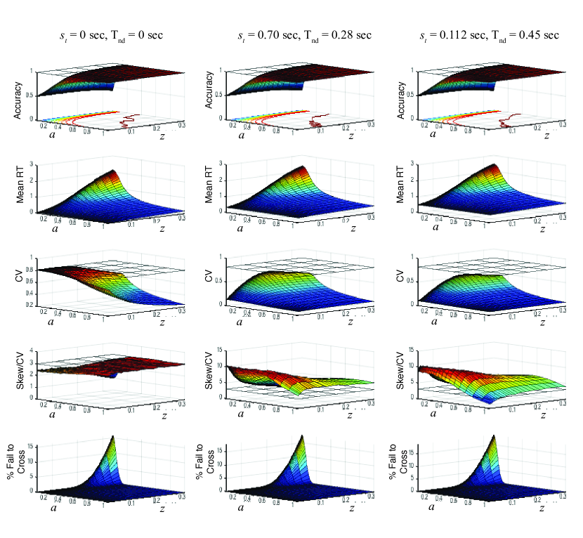
Figure 8: Effects of range $s_{t}$ of uniformly distributed $\rm T_{\textup{nd}}$. High values of $s_{t}$ (25% of $\rm T_{\textup{nd}}$) produce little effect compared with that of increasing $\rm T_{\textup{nd}}$.

The remaining figures show the effects of variability in $\rm T_{\textup{nd}}$, of starting point and its variability, and of variability in drift rates. In Fig. 8 we keep the ratio $s_{t}/\rm T_{\textup{nd}}$ constant at $0.25$ and use the same values of $\rm T_{\textup{nd}}$ as in Fig. 6, revealing similar effects to those of Fig. 6, except for SCV, which increases as $\rm T_{\textup{nd}}$ increases.

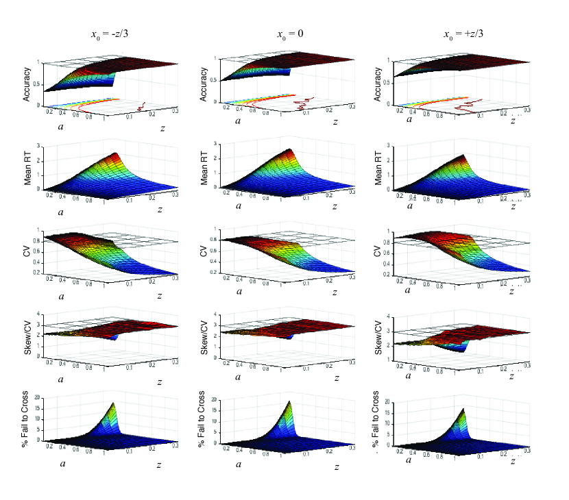
Figure 9: Effects of mean starting point $x_{0}$. Positive and negative biases from $0$ produce increases in the CV of decision times, raising it above $\sqrt{2/3}$, but with very little change in SCV. Note that $\rm T_{\textup{nd}}=0$ in all plots.

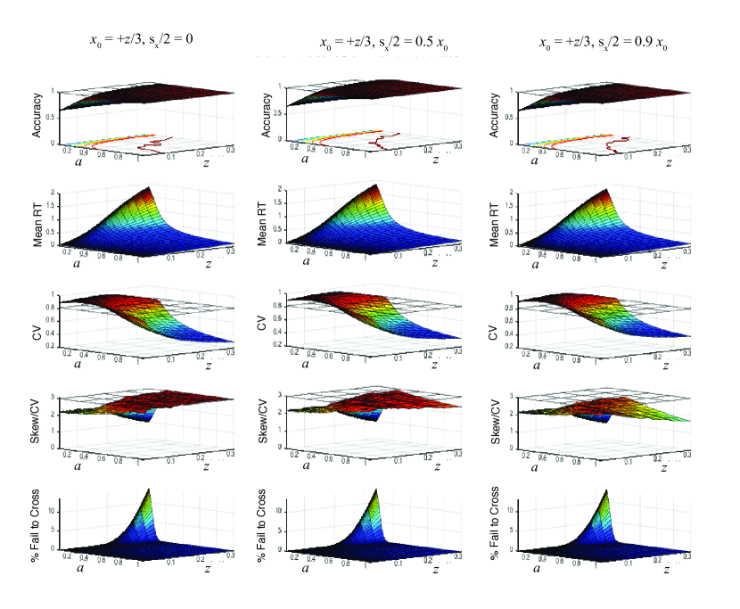
Figure 10: Effects of range of starting point distribution $s_{x}$. Increasing $s_{x}$ has little effect, except at unrealistic parameter combinations of high threshold and high drift, where a decrease in SCV is evident. Mean starting point in all plots is $+z/3$, 2/3 of distance from lower to upper threshold biased toward the correct response. Indeed, $s_{x}$ is used to explain differences in conditional decision times, and any apparent lack of effect in Fig. 10 is due to the fact that only unconditional quantities are plotted.

Figure 11: Increases in drift variability $\sigma_{a}$ across trials reduce accuracy, increase CVs, and initially raise and then lower SCV ratios; overall mean RTs are little changed.

References

- [1] M. Abramowitz and I.A. Stegun, eds. Handbook of Mathematical Functions with Formulas, Graphs, and Mathematical Tables. Wiley - Interscience, New York, 1984.
- [2] F. Balci and P. Simen. Decision processes in temporal discrimination. Acta Psychologica, 149:157–168, 2014.
- [3] F. Balci, P. Simen, R. Niyogi, A. Saxe, P. Holmes, and J.D. Cohen. Acquisition of decision making criteria: Reward rate ultimately beats accuracy. Attention, Perception & Psychophysics, 73(2):640–657, 2011.
- [4] R. Bogacz, E. Brown, J. Moehlis, P. Holmes, and J.D. Cohen. The physics of optimal decision making: A formal analysis of models of performance in two alternative forced choice tasks. Psychological Reveiw, 113 (4):700–765, 2006.
- [5] R. Bogacz, P. Hu, P. Holmes, and J.D. Cohen. Do humans produce the speed-accuracy tradeoff that maximizes reward rate? Quarterly Journal Experimental Psychology, 63(5):863–891, 2010.
- [6] A.N. Borodin and P. Salminen. Handbook of Brownian Motion: Facts and Formulae. Springer, New York, 2002.
- [7] C. D. Creelman. Human discrimination of auditory duration. The Journal of the Acoustical Society of America, 34:582–593, 1962.
- [8] G. Dutilh, J. Vandekerckhove, F. Tuerlinckx, and E-J. Wagenmakers. A diffusion model decomposition of the practice effect. Psychonomic Bulletin and Review, 16(6):1026–1036, 2009.
- [9] C. B. Ferster and B. F. Skinner. Schedules of Reinforcement. Appleton-Century-Crofts, New York, 1957.
- [10] C.W. Gardiner. Stochastic Methods: A Handbook for the Natural and Social Sciences. Springer, New York, 2009. 4th edition.
- [11] J. Gibbon and R. M. Church. Representation of time. Cognition, 37:23–54, 1990.
- [12] J. Gibbon, R. M. Church, and W. H. Meck. Scalar timing in memory. In J. Gibbon and L. G. Allan, editors, Annals of the New York Academy of Sciences: Timing and Time Perception, volume 423, pages 52–77, New York, 1984. New York Academy of Sciences.
- [13] R. P. P. P. Grasman, E-J. Wagenmakers, and H. L. J. van der Maas. On the mean and variance of response times under the diffusion model with an application to parameter estimation. Journal of Mathematical Psychology, 53(2):55–68, 2009.
- [14] G. Grimmett and D. Stirzaker. Probability and Random Processes. Oxford University Press, Oxford, UK, 2001.
- [15] A. Gut. Probability: A Graduate Course. Springer, New York, 2007. Corrected 2nd printing.
- [16] D.J. Higham. An algorithmic introduction to numerical simulation of stochastic differential equations. SIAM Review, 43:525–546, 2001.
- [17] Peter R. Killeen and J. Gregor Fetterman. A behavioral theory of timing. Psychological Review, 95(2):274–295, 1988.
- [18] R.D. Luce. Response Times: Their Role in Inferring Elementary Mental Organization. Oxford University Press, New York, 1986.
- [19] A. Luzardo, E. A. Ludvig, and F. Rivest. An adaptive drift-diffusion model of interval timing dynamics. Behavioral Processes, 95:90–99, 2013.
- [20] R. Ratcliff. A theory of memory retrieval. Psychological Review, 85:59–108, 1978.
- [21] R. Ratcliff. Methods for dealing with reaction time outliers. Psychological Bulletin, 114:510–532, 1993.
- [22] R. Ratcliff. Measuring psychometric functions with the diffusion model. Journal of Experimental Psychology: Human Perception and Performance, 40(2):870–888, 2014.
- [23] R. Ratcliff and J. N. Rouder. Modeling response times for two-choice decisions. Psychological Science, 9:347–356, 1998.
- [24] R. Ratcliff and P.L. Smith. A comparison of sequential sampling models for two-choice reaction time. Psychological Review, 111:333–367, 2004.
- [25] P. Simen, F. Balci, L. deSouza, J.D. Cohen, and P. Holmes. A model of interval timing by neural integration. Journal of Neuroscience, 31(25):9238–9253, 2011.
- [26] P. Simen, D. Contreras, C. Buck, P. Hu, P. Holmes, and J.D. Cohen. Reward rate optimization in two-alternative decision making: Empirical tests of theoretical predictions. Journal of Experimental Psychology: Humam Perception Performance, 35(6):1865–1897, 2009.
- [27] P. Simen, F. Rivest, E. A. Ludvig, F. Balci, and P. R. Killeen. Timescale invariance in the pacemaker-accumulator family of timing models. Timing and Time Perception, 1:159–188, 2013.
- [28] P. Simen, K. Vlasov, and S. Papadakis. Scale (in)variance in a unified diffusion model of decision making and timing. Psychological Review, 2016.
- [29] M. Treisman. Temporal discrimination and the indifference interval: implications for a model of the ‘internal clock’. Psychological Monographs, 77:1–31, 1963.
- [30] J. Vandekerckhove and F. Tuerlinckx. Fitting the ratcliff diffusion model to experimental data. Psychonomic Bulletin & Review, 14(6):1011–1026, 2007.
- [31] S. Verdonck, K. Meers, and F. Tuerlinckx. Efficient simulation of diffusion-based choice rt models on CPU and GPU. Behavior Research Methods, pages 1–15, 2015.
- [32] E-J. Wagenmakers, R. P. P. P. Grasman, and P. C. M. Molenaar. On the relation between the mean and the variance of a diffusion model response time distribution. Journal of Mathematical Psychology, 49:195–204, 2005.
- [33] A. Wald. Sequential Analysis. John Wiley & Sons, New York, 1947.