A Simple Accurate Method for Solving Fractional Variational and Optimal Control Problems

Abstract

We develop a simple and accurate method to solve fractional variational and fractional optimal control problems with dependence on Caputo and Riemann–Liouville operators. Using known formulas for computing fractional derivatives of polynomials, we rewrite the fractional functional dynamical optimization problem as a classical static optimization problem. The method for classical optimal control problems is called Ritz’s method. Examples show that the proposed approach is more accurate than recent methods available in the literature.

1 Introduction

In view of its history, fractional (non-integer order) calculus is as old as the classical calculus MR2218073 ; MR1347689 ; MR3181071 . Roughly speaking, there is just one definition of fractional integral operator, which is the Riemann–Liouville fractional integral. There are, however, several definitions of fractional differentiation, e.g., Caputo, Riemann–Liouville, Hadamard, and Wily differentiation MR3224387 ; MR2960307 . Each type of fractional derivative has its own properties, which make richer the area of fractional calculus and enlarge its range of applicability MR2768178 ; MR3188372 .

There are two recent research areas where fractional operators have a particularly important role: the fractional calculus of variations and the fractional theory of optimal control sal34 ; book:adv:FCV ; MR2984893 . A fractional variational problem is a dynamic optimization problem, in which the objective functional, as well as its constraints, depends on derivatives or integrals of fractional order, e.g., Caputo, Riemann–Liouville or Hadamard fractional operators. This is a generalization of the classical theory, where derivatives and integrals can only appear in integer orders. If at least one non-integer (fractional) term exists in its formulation, then the problem is said to be a fractional variational problem or a fractional optimal control problem. The theory of the fractional calculus of variations was introduced by Riewe in 1996, to deal with nonconservative systems in mechanics sal1 ; sal2 . This subject has many applications in physics and engineering, and provides more accurate models of physical phenomena. For this reason, it is now under strong development: see sal5 ; sal3 ; sal4 ; MR3103208 ; MR3162654 ; MR3200762 and the references therein. For a survey, see MR3221831 .

There are two main approaches to solve problems of the fractional calculus of variations or optimal control. One involves solving fractional Euler–Lagrange equations or fractional Pontryagin-type conditions, which is the indirect approach; the other involves addressing directly the problem, without involving necessary optimality conditions, which is the direct approach. The emphasis in the literature has been put on indirect methods book:adv:FCV ; MR2984893 ; sal6 ; sal7 . For direct methods, see sal34 ; sal3 . Furthermore, Almeida et al. developed direct numerical methods based on the idea of writing the fractional operators in power series, and then approximating the fractional problems with classical ones MyID:294 ; sal8 . In this paper, we use a different approach to solve fractional variational problems and fractional optimal control problems, based on Ritz’s direct method. The idea is to restrict admissible functions to linear combinations of a set of known basis functions. We choose basis functions in such a way that the approximated function satisfies the given boundary conditions. Using the approximated function and its derivatives whenever needed, we transform the functional into a multivariate function of unknown coefficients. Recently, Dehghan et al. in sal9 used the Rayleigh–Ritz method, based on Jacobi polynomials, to solve fractional optimal control problems. Several illustrative examples show that our results are more accurate and more useful than the ones introduced in sal8 ; sal9 .

The paper is organized as follows. In Section 2, we present some necessary preliminaries on fractional calculus. In Section 3, we investigate Ritz’s method for solving three kinds of fractional variational problems. In Section 4, we solve five examples of fractional variational problems and three examples of fractional optimal control problems, comparing our results with previous methods available in the literature. The main conclusions are given in Section 5.

2 Preliminaries and Notations About Fractional Calculus

Riemann–Liouville fractional integrals are a generalization of the $n$ fold integral, $n\in\mathbb{N}$, to real value numbers. Using the usual notation in the theory of fractional calculus, we define the Riemann–Liouville fractional integrals as follows.

Definition 1 (Fractional integrals)

The left and right Riemann–Liouville fractional integrals of order $\alpha>0$ of a given function $f$ are defined by

$${}_{a}I_{x}^{\alpha}f(x):=\frac{1}{\Gamma(\alpha)}\int_{a}^{x}(x-t)^{\alpha-1}f(t)dt$$

and

$${}_{x}I_{b}^{\alpha}f(x):=\frac{1}{\Gamma(\alpha)}\int_{x}^{b}(t-x)^{\alpha-1}f(t)dt,$$

respectively, where $\Gamma$ is Euler’s gamma function, that is,

$$\Gamma(x):=\int_{0}^{\infty}t^{x-1}e^{-t}dt,$$

and $a<x<b$.

The left Riemann–Liouville fractional operator has the following properties:

$${{}_{a}I_{x}^{\alpha}}{{}_{a}I_{x}^{\beta}}={{}_{a}I_{x}}^{\alpha+\beta},\quad{{}_{a}I_{x}^{\alpha}}{{}_{a}I_{x}^{\beta}}={{}_{a}I_{x}^{\beta}}{{}_{a}I_{x}^{\alpha}},$$

$$_{a}I_{x}^{\alpha}(x-a)^{n}=\frac{\Gamma(n+1)}{\Gamma(\alpha+n+1)}(x-a)^{\alpha+n},\quad x>a,$$ (1)

where $\alpha,\beta\geq 0$ and $n\in\mathbb{N}_{0}=\{0,1,\ldots\}$. Similar relations hold for the right Riemann–Liouville fractional operator. Now, using the definition of fractional integral, we define two kinds of fractional derivatives.

Definition 2 (Riemann–Liouville derivatives)

Let $\alpha>0$ with $n-1<\alpha\leq n$, $n\in\mathbb{N}$. The left and right Riemann–Liouville fractional derivatives of order $\alpha>0$ of a given function $f$ are defined by

$${}_{a}D_{x}^{\alpha}f(x):=D^{n}(_{a}I_{x}^{n-\alpha})f(x)=\frac{1}{\Gamma(n-\alpha)}\frac{d^{n}}{dx^{n}}\int_{a}^{x}(x-t)^{n-\alpha-1}f(t)dt$$

and

$${}_{x}D_{b}^{\alpha}f(x):=(-1)^{n}D^{n}(_{x}I_{b}^{n-\alpha})f(x)=\frac{(-1)^{n}}{\Gamma(n-\alpha)}\frac{d^{n}}{dx^{n}}\int_{x}^{b}(t-x)^{n-\alpha-1}f(t)dt,$$

respectively.

The following relations hold for the left Riemann–Liouville fractional derivative:

$${{}_{a}D_{x}^{\alpha}}{{}_{a}D_{x}^{\beta}}={{}_{a}D_{x}}^{\alpha+\beta},\quad{{}_{a}D_{x}^{\alpha}}{{}_{a}D_{x}^{\beta}}={{}_{a}D_{x}^{\beta}}{{}_{a}D_{x}^{\alpha}},$$

$${}_{a}D_{x}^{\alpha}k=\frac{k(x-a)^{\alpha}}{\Gamma(1-\alpha)},$$

$$_{a}D_{x}^{\alpha}(x-a)^{n}=\frac{\Gamma(n+1)}{\Gamma(n-\alpha+1)}(x-a)^{n-\alpha},\quad x>a,$$ (2)

where $\alpha,\beta\geq 0$, $k$ is a constant and $n\in\mathbb{N}_{0}$. Similar relations hold for the right Riemann–Liouville fractional derivative.

Another type of fractional derivative, which also uses the Riemann–Liouville fractional integral in its definition, was proposed by Caputo sal16 .

Definition 3 (Caputo derivatives)

Let $\alpha>0$ with $n-1<\alpha\leq n$, $n\in\mathbb{N}$. The left and right Caputo fractional derivatives of order $\alpha>0$ of a given function $f$ are defined by

$${}_{a}^{C}D_{x}^{\alpha}f(x):=(_{a}I_{x}^{n-\alpha})D^{n}f(x)=\frac{1}{\Gamma(n-\alpha)}\int_{a}^{x}(x-t)^{n-\alpha-1}f^{(n)}(t)dt$$

and

$${}_{x}^{C}D_{b}^{\alpha}f(x):=(-1)^{n}(_{x}I_{b}^{n-\alpha})D^{n}f(x)=\frac{(-1)^{n}}{\Gamma(n-\alpha)}\int_{x}^{b}(t-x)^{n-\alpha-1}f^{(n)}(t)dt,$$

respectively.

The following relations hold for the left Caputo fractional derivative:

$${{}_{a}^{C}D_{x}^{\alpha}}\,{{}_{a}^{C}D_{x}^{\beta}}={{{}_{a}^{C}D_{x}^{\alpha+\beta}}},\quad{{}_{a}^{C}D_{x}^{\alpha}}\,{{}_{a}^{C}D_{x}^{\beta}}={{}_{a}^{C}D_{x}^{\beta}}\,{{}_{a}^{C}D_{x}^{\alpha}},$$

$${}_{a}^{C}D_{x}^{\alpha}k=0,$$

$$_{a}^{C}D_{x}^{\alpha}(x-a)^{n}=\left\{\begin{array}[]{ll}\frac{\Gamma(n+1)}{\Gamma(n-\alpha+1)}(x-a)^{n-\alpha},&n\geq[\alpha],\\ 0,&n<[\alpha],\end{array}\right.$$ (3)

where $\alpha,\beta\geq 0$, $k$ is a constant, $x>a$, $n\in\mathbb{N}_{0}$, and $[\cdot]$ is the ceiling function, that is, $[\alpha]$ is the smallest integer greater than or equal to $\alpha$. Similar relations hold for the right Caputo fractional derivative. Moreover, the following relations between Caputo and Riemann–Liouville fractional derivatives hold:

$${}_{a}^{C}D_{x}^{\alpha}f(x)={{}_{a}D_{x}^{\alpha}}f(x)-\sum_{k=0}^{n-1}\frac{f^{(k)}(a)}{\Gamma(k-\alpha+1)}(x-a)^{k-\alpha}$$

and

$${}_{x}^{C}D_{b}^{\alpha}f(x)={{}_{x}D_{b}^{\alpha}}f(x)-\sum_{k=0}^{n-1}\frac{f^{(k)}(b)}{\Gamma(k-\alpha+1)}(b-x)^{k-\alpha}.$$

Therefore, if $f\in C^{n}[a,b]$ and $f^{(k)}(a)=0$, $k=0,1,\ldots,n-1$, then ${}_{a}^{C}D_{x}^{\alpha}f={{}_{a}D_{x}^{\alpha}}f$; if $f^{(k)}(b)=0$, $k=0,1,\ldots,n-1$, then ${}_{x}^{C}D_{b}^{\alpha}f={{}_{x}D_{b}^{\alpha}}f$.

3 Main Results

Consider the following fractional variational problem: find $y\in C^{n}[a,b]$ in such a way to minimize or maximize the functional

$$J\{y\}=\int_{a}^{b}L(t,y(t),D^{\alpha}y(t))dt,\quad n-1\leq\alpha<n,$$ (4)

subject to boundary conditions

$$y^{(k)}(a)=u_{k,a},\quad y^{(k)}(b)=u_{k,b},\quad k=0,1,\ldots,n-1,$$ (5)

where $L$ is the Lagrangian, assumed to be continuous with respect to all its arguments, $D^{\alpha}$ is a fractional operator (left or right Riemann–Liouville fractional integral or derivative or left or right Caputo fractional derivative), and $u_{k,a}$ and $u_{k,b}$, $k=0,1,\ldots,n-1$, are given constants. To solve problem (4)–(5) with our method, we need to recall the following classical theorems from approximation theory.

Theorem 3.1 (Stone–Weierstrass theorem (1937))

Let $K$ be a compact metric space and $A\subset C(K,R)$ a unital sub-algebra, which separates points of $K$. Then, $A$ is dense in $C(K,R)$.

Theorem 3.2 (Weierstrass approximation theorem (1885))

If $f\in C([a,b],\mathbb{R})$, then there is a sequence of polynomials $P_{n}(x)$ that converges uniformly to $f(x)$ on $[a,b]$.

Theorem 3.3

Let $P_{N}(x):=\sum_{i=0}^{N}c_{i}(x-a)^{i}$ be a polynomial. Then,

$$_{a}I_{x}^{\alpha}P_{N}(x)=\sum_{i=0}^{N}c_{i}\frac{\Gamma(i+1)}{\Gamma(\alpha+i+1)}(x-a)^{\alpha+i},$$ (6)

$$_{a}D_{x}^{\alpha}P_{N}(x)=\sum_{i=0}^{N}c_{i}\frac{\Gamma(i+1)}{\Gamma(i-\alpha+1)}(x-a)^{i-\alpha},$$ (7)

$$_{a}^{C}D_{x}^{\alpha}P_{N}(x)=\sum_{i=[\alpha]}^{N}\frac{\Gamma(i+1)}{\Gamma(i-\alpha+1)}(x-a)^{i-\alpha},$$ (8)

for $x>a$.

Proof

Follows from relations (1), (2) and (3) and the linearity property of the fractional operators. ∎

For solving fractional variational problems involving right fractional operators, we use the following theorem.

Theorem 3.4

Let $P_{N}(x):=\sum_{i=0}^{N}c_{i}(b-x)^{i}$ be a polynomial. Then,

$$_{x}I_{b}^{\alpha}P_{N}(x)=\sum_{i=0}^{N}c_{i}\frac{\Gamma(i+1)}{\Gamma(\alpha+i+1)}(b-x)^{\alpha+i},$$ (9)

$$_{x}D_{b}^{\alpha}P_{N}(x)=\sum_{i=0}^{N}c_{i}\frac{\Gamma(i+1)}{\Gamma(i-\alpha+1)}(b-x)^{i-\alpha},$$ (10)

$$_{x}^{C}D_{b}^{\alpha}P_{N}(x)=\sum_{i=[\alpha]}^{N}\frac{\Gamma(i+1)}{\Gamma(i-\alpha+1)}(b-x)^{i-\alpha},$$ (11)

for $x<b$.

Proof

Similar to the proof of Theorem 3.3. ∎

Without any loss of generality, from now on we consider $a=0$, $b=1$ and $t\in[0,1]$ in the fractional variational problem (4)–(5).

3.1 Fractional Variational Problems Involving Left Operators

Consider the fractional variational functional (4) involving a left fractional operator, subject to boundary conditions (5). To find the function $y(x)$ that solves problem (4)–(5), we put

$$y(x)\simeq y_{N}(x)=\sum_{i=0}^{N}c_{i}x^{i}.$$ (12)

Then, by substituting (12) and relations (6)–(8) into (4), we obtain

$$J[y]=J[c_{0},c_{1},\ldots,c_{N}]=\int_{0}^{1}L(x,y_{N}(x),D^{\alpha}y_{N}(x))dx$$ (13)

subject to boundary conditions

$$y_{N}^{(k)}(0)=u_{k,0},\quad y_{N}^{(k)}(1)=u_{k,1},\quad k=0,1,\ldots,n-1,$$ (14)

which is an algebraic function of unknowns $c_{i}$, $i=0,1,\ldots,N$. To optimize the algebraic function $J$, we act as follows. We should find $c_{0},c_{1},\ldots,c_{N}$, such that $y_{N}$ satisfies boundary conditions (14). This means that the following relations must be satisfied:

$$y_{N}^{(k)}(0)=u_{k,0},\quad y_{N}^{(k)}(1)=u_{k,1},\quad k=0,1,\ldots,n-1.$$ (15)

Using the well known Hermite interpolation and the relations (15), we calculate $c_{0},c_{1},\ldots,c_{n}$. For obtaining the values of $c_{n+1},c_{n+2},\ldots,c_{N}$, firstly we use the $N+1$ point Gauss–Legendre quadrature rule, which is exact for every polynomial of degree up to $2N+2$. Secondly, we calculate the exact value of the integral in the right-hand side of (13). Then, according to differential calculus, we must solve the following system of equations:

$$\frac{\partial J}{\partial c_{j}}=0,\quad j=n+1,n+2,\ldots,N,$$ (16)

which, depending on the form of $L$, is a linear or nonlinear system of equations. Furthermore, we choose the value of $N$ such that $|y_{N+1}(x)-y_{N}(x)|\cong 0(x)$, where $0(x)$ is the null polynomial.

3.2 Fractional Variational Problems Involving Right Operators

Now consider the fractional variational functional (4) involving a right fractional operator, subject to boundary conditions (5). To find function $y(x)$ that solves problem (4)–(5), we put

$$y(x)\simeq y_{N}(x)=\sum_{i=0}^{N}c_{i}(1-x)^{i}.$$ (17)

Then, substituting (17) and relations (9)–(11) into (4), we obtain

$$J[y]=J[c_{0},c_{1},\ldots,c_{N}]=\int_{0}^{1}L(x,y_{N}(x),D^{\alpha}y_{N}(x))dx$$ (18)

subject to boundary conditions

$$y_{N}^{(k)}(0)=u_{k,0},\quad y_{N}^{(k)}(1)=u_{k,1},\quad k=0,1,\ldots,n-1,$$

which is an algebraic function of unknowns $c_{i}$, $i=0,1,\ldots,N$. To optimize the algebraic function (18), we act as explained in Section 3.1.

3.3 Fractional Optimal Control Problems

A fractional optimal control problem requires finding a control function $u(t)$ and the corresponding state trajectory $x(t)$, that minimizes (or maximizes) a given functional

$$J\{x,u\}=\int_{a}^{b}L\left(t,x(t),u(t)\right)dt$$ (19)

subject to a fractional dynamical control system

$$D^{\alpha}x(t)=f(t,x(t),u(t))$$ (20)

and boundary conditions

$$x^{(k)}(a)=u_{k,a},\quad x^{(k)}(b)=u_{k,b},\quad k=0,1,\ldots,n-1,$$ (21)

where $D^{\alpha}$ is a fractional operator, $\alpha$ is a positive real number, and $f$ and $L$ are two known functions. For more details, see MyID:294 ; sal14 ; MR2433010 ; MR2386201 ; sal15 and the references therein.

Here we restrict our attention to those fractional optimal control problems (19)–(21), for which one can solve (20) with respect to $u$ and write

$$u(t)=g\left(t,x(t),D^{\alpha}x(t)\right).$$ (22)

Then, by substituting (22) into (19), we obtain the following fractional variational problem (FVP): find function $x(t)$ that extremizes the functional

$$J\{x\}=\int_{a}^{b}L\left(t,x(t),g(t,x(t),D^{\alpha}x(t))\right)dt$$ (23)

subject to boundary conditions

$$x^{(k)}(a)=u_{k,a},\quad x^{(k)}(b)=u_{k,b},\quad k=0,1,\ldots,n-1.$$ (24)

We solve the FVP (23)–(24) by using the method illustrated in previous sections, and then we find control function $u(t)$ by using (22).

Remark 1

Similarly to classical Ritz’s method, the trial functions are selected to meet boundary conditions (and any other constraints). The exact solutions are not known; and the trial functions are parametrized by adjustable coefficients, which are varied to find the best approximation for the basis functions used. The choice of the basis functions depends on the solution space. Since our problems involve finding $C^{n}$ solutions, we choose the basis functions to be polynomials. If the solution space is another one, like the $L_{p}$ space or the space of harmonic functions, then we should choose some basis functions like Fourier or wavelet basis.

Remark 2

For choosing the number $N$ one needs to decide on the required accuracy. One can stop when the difference between two consecutive approximations $y_{N}$ and $y_{N-1}$ or their respective functional values is smaller than a desired tolerance, that is, when $\left\|y_{N}-y_{N-1}\right\|\leq\varepsilon$ or when $\left|J[y_{N}]-J[y_{N-1}]\right|\leq\varepsilon$ for some given $\varepsilon$. Note that for a minimization (maximization) problem, the functional $J$ is always a non-increasing (non-decreasing) function of $N$: $J[y_{N}]\leq J[y_{N-1}]$ ($J[y_{N}]\geq J[y_{N-1}]$). Moreover, if $y$ is the (unknown) exact solution of the fractional variational problem at hand, then $y_{N}$ converges uniformly to $y$ (Theorems 3.1 and 3.2).

Remark 3

Throughout the paper, $N$ is greater than $n$.

In the next section, we solve five fractional problems of the calculus of variations and three fractional optimal control problems. Six of the eight problems involve left fractional operators, while the other two involve right operators.

4 Illustrative Examples

We begin by solving two problems of the calculus of variations involving a left Riemann–Liouville fractional derivative. These problems were recently investigated by Almeida et al. in sal34 . We also solve three examples involving left and right Caputo fractional derivatives, which were recently considered by Dehghan et al. in sal9 , and we compare the results. Finally, we solve three fractional optimal control problems that were investigated before in MyID:294 ; sal15 ; sal17 . For all examples, the error between the exact solution $y$ and the approximate solution $y_{N}$, found using our method, is computed as follows:

$$Error\{y,y_{N}\}=\int_{0}^{1}(y(x)-y_{N}(x))^{2}dx.$$ (25)

The results show that our method is very simple but very accurate, providing better results than those found in the literature.

Example 1

sal34 ; sal8 Let $\alpha\in]0,1[$. Consider the following FVP:

$$\text{minimize}\quad J\{y\}=\int_{0}^{1}\left({}_{0}D_{x}^{\alpha}y(x)-(y^{\prime})^{2}(x)\right)dx,$$ (26)

subject to

$$y(0)=0,\quad y(1)=1.$$ (27)

The exact solution to problem (26)–(27) is

$$y(x)=-\frac{1}{2\Gamma(3-\alpha)}(1-x)^{2-\alpha}+\left(1-\frac{1}{2\Gamma(3-\alpha)}\right)x+\frac{1}{2\Gamma(3-\alpha)}$$

sal34 ; sal8 . With the given boundary conditions (27), we consider

$$y_{N}(x)=\left(1-\sum_{i=2}^{N}c_{i}\right)x+\sum_{i=2}^{N}c_{i}x^{i}.$$

Using our method, we calculate the $c_{i}$’s by solving the system of equations (16). For $\alpha=0.5$ and $N=2$, we have

$$y(x)=0.376126-0.376126(1-x)^{1.5}+0.623874x,$$

$$y_{2}(x)=1.22568x-0.225676x^{2}.$$

Figure 1 plots the result for $\alpha=0.5$ and $N=2$. The errors computed with (25) for different values of $\alpha$ and $N$ are presented in Table 1.

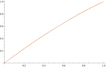
Figure 1: Exact solution to problem (26)–(27) of Example 1 with $\alpha=0.5$ (the solid line) versus our approximate solution with $N=2$ (the dashed line).

Table 1: Errors obtained for problem (26)–(27) of Example 1 when computed with (25) for $\alpha=0.25,0.5,0.75$ and $N=3,4,5,6$.

$\alpha$	$N=3$	$N=4$	$N=5$	$N=6$
$0.25$	$1.7\times 10^{-7}$	$1.9\times 10^{-8}$	$3.6\times 10^{-9}$	$9.1\times 10^{-10}$
$0.5$	$9.7\times 10^{-6}$	$1.5\times 10^{-7}$	$3.5\times 10^{-8}$	$1.1\times 10^{-8}$
$0.75$	$1.6\times 10^{-6}$	$3.4\times 10^{-7}$	$9.9\times 10^{-8}$	$3.5\times 10^{-8}$

Our approximate results are better than the ones presented in sal34 ; sal8 .

Example 2

sal34 Let $\alpha=0.5$ and consider the minimization problem

$$\text{minimize}\quad J\{y\}=\int_{0}^{1}\left({}_{0}D_{x}^{\alpha}y(x)-\frac{16\Gamma(6)}{\Gamma(5.5)}x^{4.5}+\frac{20\Gamma(4)}{\Gamma(3.5)}x^{2.5}-\frac{5}{\Gamma(2.5)}x^{0.5}\right)^{4}dx,$$ (28)

subject to the boundary conditions

$$y(0)=0,\quad y(1)=1.$$ (29)

The minimizer to the FVP (28)–(29) is given by $y(x)=16x^{5}-20x^{3}+5x$. For $N=5$, we obtain

$$y_{5}(x)=5x+(2.3995\times 10^{-10})x^{2}{-20}x^{3}+(7.70126\times 10^{-10})x^{4}+16x^{5}.$$

Figure 2 shows that our results are more accurate than the results presented in sal34 .

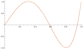
(a) $N=4$

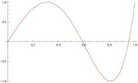
(b) $N=5$

Figure 2: Exact solution to problem (28)–(29) of Example 2 (the solid line) versus our approximate solutions with $N=4,5$ (the dashed line).

Below we solve three problems of the calculus of variations, which were recently solved by Dehghan et al. in sal9 . Our results show that our method is also more accurate than the method introduced in sal9 .

Example 3

sal9 Consider the following FVP:

$$\text{minimize}\quad J\{y\}=\frac{1}{2}\int_{0}^{1}(_{0}^{C}D_{x}^{\alpha}y(x)-f(x))^{2}dx,\quad 0<\alpha<1,$$ (30)

where $f(x)$ is given by

$$f(x)=\frac{\Gamma(\beta+1)}{\Gamma(1+\beta-\alpha)}x^{\beta-\alpha},$$

subject to the boundary conditions

$$y(0)=0,\quad y(1)=1.$$ (31)

The exact solution to this problem is $y(x)=x^{\beta}$ sal9 . In Figure 3, the exact solution for $\alpha=0.5$ and $\beta=2.5$ versus our numerical solution for $N=3$ is plotted. Note that for $\beta=k$, $k\in\mathbb{N}$, the error is equal to zero when $N\geq k$.

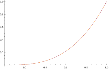
Figure 3: Exact solution to problem (30)–(31) of Example 3 with $\alpha=0.5$ and $\beta=2.5$ (the solid line) versus our approximate solution with $N=3$ (the dashed line).

Example 4

sal9 Consider the following FVP, depending on a right Caputo fractional derivative:

$$\text{minimize}\quad J\{y\}=\frac{1}{2}\int_{0}^{1}(_{x}^{C}D_{1}^{\alpha}y(x)-1)^{2}dx,\quad 0<\alpha<1,$$ (32)

subject to boundary conditions

$$y(0)=1+\frac{1}{\Gamma(1+\alpha)},\quad y(1)=1.$$ (33)

The exact solution to (32)–(33) is given by

$$y(x)=1+\frac{(1-x)^{\alpha}}{\Gamma(1+\alpha)}.$$

An approximate solution obtained with our method is shown in Figure 4. See Table 2 for the error of our approximations.

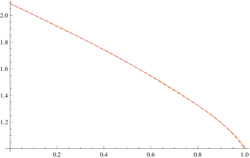
Figure 4: Exact solution to problem (32)–(33) of Example 4 with $\alpha=0.75$ (the solid line) versus our approximate solution with $N=6$ (the dashed line).

Table 2: Errors obtained for problem (32)–(33) of Example 4, computed with (25) for $\alpha=0.75$ and $N=2,3,4,5,6$.

$\alpha$	$N=2$	$N=3$	$N=4$	$N=5$	$N=6$
$0.75$	$5.7\times 10^{-4}$	$1.2\times 10^{-4}$	$3.6\times 10^{-5}$	$1.6\times 10^{-5}$	$7.2\times 10^{-6}$

Example 5

sal9 As a second example involving a fractional right operator, consider the following FVP with $0<\alpha<1$:

$$\text{minimize}\quad J\{y\}=\int_{0}^{1}\left({}_{x}^{C}D_{1}^{\alpha}y(x)+y(x)-(1-x)^{\beta}-\frac{\Gamma(\beta+1)(1-x)^{\beta-\alpha}}{\Gamma(\beta-\alpha+1)}\right)^{2}dx,$$ (34)

subject to boundary conditions

$$y(0)=1,\quad y(1)=0.$$ (35)

In this case the exact solution is $y(x)=(1-x)^{\beta}$ sal9 . Figure 5 shows the exact solution for $\alpha=0.39$ and $\beta=3$ versus our numerical solution with $N=3$. The errors (25) of our approximations, for different values of $(\alpha,\beta)$, $\beta\neq 3$, are listed in Table 3. As with Example 3, the error for $\beta=k$, $k\in\mathbb{N}$, is equal to zero when we consider $N\geq k$.

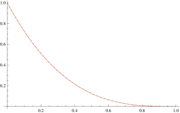
Figure 5: Exact solution to problem (34)–(35) of Example 5 with $\alpha=0.39$ and $\beta=3$ (the solid line) versus our approximate solution with $N=3$ (the dashed line).

Table 3: Errors for problem (34)–(35) of Example 5 when computed with (25) for different values of $(\alpha,\beta)$ and $N=3,4,5$.

$(\alpha,\beta)$	$N=3$	$N=4$	$N=5$
$(0.39,1.5)$	$6.1\times 10^{-6}$	$8.1\times 10^{-7}$	$1.7\times 10^{-8}$
$(0.39,2.5)$	$1.3\times 10^{-6}$	$4.5\times 10^{-8}$	$3.7\times 10^{-9}$
$(0.59,1.5)$	$6.2\times 10^{-6}$	$8.1\times 10^{-7}$	$4.5\times 10^{-9}$
$(0.59,2.5)$	$1.3\times 10^{-6}$	$4.5\times 10^{-8}$	$4.5\times 10^{-9}$

We finish by applying our method to three fractional optimal control problems.

Example 6

sal15 ; sal17 Consider the following fractional optimal control problem (FOCP):

$$\text{minimize}\quad J\{x,u\}=\int_{0}^{1}(tu(t)-(\alpha+2)x(t))^{2}dt,$$ (36)

subject to the dynamical fractional control system

$$x^{\prime}(t)+{{}_{0}^{C}D_{t}^{\alpha}}x(t)=u(t)+t^{2}$$ (37)

and the boundary conditions

$$x(0)=0,\quad x(1)=\frac{2}{\Gamma(3+\alpha)}.$$ (38)

The exact solution is given by

$$(x(t),u(t))=\left(\frac{2t^{\alpha+2}}{\Gamma(\alpha+3)},\frac{2t^{\alpha+1}}{\Gamma(\alpha+2)}\right).$$

To solve this problem with our method, we take

$$x_{N}(t)=\left(\frac{2}{\Gamma(3+\alpha)}-\sum_{i=1}^{N}c_{i}\right)t+\sum_{i=1}^{N}c_{i}t^{i}.$$

The results for $\alpha=0.5$ and $N=3,4$ are plotted in Figure 6. Table 4 shows the errors for $\alpha=0.5$ and $N=2,3,4$.

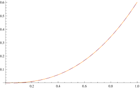
(a) $x(t)$, $N=3$

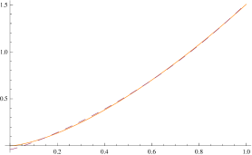
(b) $u(t)$, $N=3$

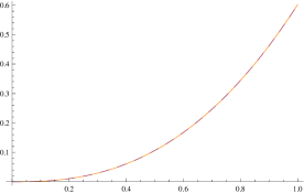
(c) $x(t)$, $N=4$

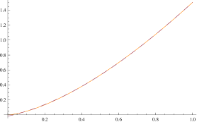
(d) $u(t)$, $N=4$

Figure 6: Exact solution $(x(t),u(t))$ to the FOCP (36)–(38) of Example 6 with $\alpha=0.5$ (the solid line) versus our approximate solution with $N=3,4$ (the dashed line).

Table 4: Errors for problem (36)–(38) of Example 6 when computed with (25) for $\alpha=0.5$ and $N=2,3,4$.

Errors	$N=2$	$N=3$	$N=4$
$Error\{x,x_{N}\}$	$1.2\times 10^{-4}$	$7.1\times 10^{-7}$	$2.8\times 10^{-8}$
$Error\{u,u_{N}\}$	$7.1\times 10^{-3}$	$9.6\times 10^{-5}$	$7.9\times 10^{-6}$

Example 7

sal17 Consider now the following FOCP:

$$\text{minimize}\quad J\{x,u\}=\int_{0}^{1}(u(t)-x(t))^{2}dt,$$ (39)

subject to the fractional dynamical control system

$$x^{\prime}(t)+{{}_{0}^{C}D_{t}^{\alpha}}x(t)=u(t)-x(t)+\frac{6t^{\alpha+2}}{\Gamma(\alpha+3)}+t^{3}$$ (40)

and the boundary conditions

$$x(0)=0,\quad x(1)=\frac{6}{\Gamma(4+\alpha)}.$$ (41)

The exact solution to (39)–(41) is given by

$$(x(t),u(t))=\left(\frac{6t^{\alpha+3}}{\Gamma(\alpha+4)},\frac{6t^{\alpha+3}}{\Gamma(\alpha+4)}\right).$$

To solve problem (39)–(41) with our method, we take

$$x_{N}(t)=\left(\frac{6}{\Gamma(4+\alpha)}-\sum_{i=1}^{N}c_{i}\right)t+\sum_{i=1}^{N}c_{i}t^{i}.$$

The results for $\alpha=0.5$ and $N=3,4$ are plotted in Figure 7. The errors (25) for $\alpha=0.5$ and $N=2,3,4$ are shown in Table 5.

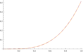
(a) $x(t)$, $N=3$

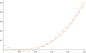
(b) $u(t)$, $N=3$

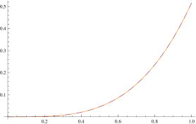
(c) $x(t)$, $N=4$

(d) $u(t)$, $N=4$

Figure 7: Exact solution $(x(t),u(t))$ to the FOCP (39)–(41) of Example 7 with $\alpha=0.5$ (the solid line) versus our approximate solution with $N=3,4$ (the dashed line).

Table 5: Errors for problem (39)–(41) of Example 7 when computed with (25) for $\alpha=0.5$ and $N=2,3,4$.

Errors	$N=2$	$N=3$	$N=4$
$Error\{x,x_{N}\}$	$7.3\times 10^{-4}$	$2.5\times 10^{-6}$	$8.4\times 10^{-9}$
$Error\{u,u_{N}\}$	$5.2\times 10^{-2}$	$3.9\times 10^{-4}$	$2.2\times 10^{-6}$

In MyID:294 the authors propose a direct method for solving fractional optimal control problems, which involves approximating the initial fractional order problem by a new one with integer order derivatives only. The latter problem is then discretized, by application of finite differences, and solved numerically. Our method is simpler and does not involve the solution of a nonlinear programming problem through AMPL and IPOPT. Moreover, as we see next, it provides a much better result when compared with the example given in MyID:294 .

Example 8

MyID:294 Consider the FOCP of MyID:294 :

$$\mathrm{minimize}\quad J\{x,u\}=\int_{0}^{1}(u^{2}(t)-4x(t))^{2}dt,$$ (42)

subject to the control system

$$x^{\prime}(t)+{{}_{0}^{C}D_{t}^{0.5}}x(t)=u(t)+\frac{2}{\Gamma(2.5)}t^{1.5},\quad t\in[0,1],$$ (43)

and the boundary conditions

$$x(0)=0,\quad\text{and}\quad x(1)=1.$$ (44)

The exact solution to (42)–(44) is given by

$$(x(t),u(t))=(t^{2},2t)$$

(see MyID:294 ). To solve problem (42)–(44) with the method of this paper, we take

$$x_{N}(t)=\left(1-\sum_{i=1}^{N}c_{i}\right)t+\sum_{i=1}^{N}c_{i}t^{i}.$$

In this case our method gives the exact solution $x(t)=t^{2}$ for $N=2$. This is in contrast with the results in MyID:294 , for which the exact solution is not found. In fact, our method provides here better results with just 2 steps ($c_{1}=0$ and $c_{2}=1$) than the method introduced in MyID:294 with 100 steps.

Remark 4

According to relations (12) and (17), accuracy depends on $N$. When the order $\alpha$ of the derivative changes, then the problem under consideration also changes. We were not able to find any general relation between $\alpha$ and the accuracy, that is, a general pattern on how $N$ changes with $\alpha$, for a fixed precision. This seems to depend on the particular situation at hand.

5 Conclusions

We introduced a numerical method, based on Ritz’s direct method, to solve problems of the fractional calculus of variations and fractional optimal control. The idea of this approach is simple: by using some known basis functions, we construct an approximate solution, which is a linear combination of the basis functions, carrying out a finite-dimensional minimization among such linear combinations and approximating the exact solution of the fractional optimal control problem. From the simulation results, the proposed approach is surprisingly accurate, and the approximate solution is nearly a perfect match with the exact solution, which is superior to the results from previous numerical methods available in the literature.

- (1) Kilbas, A.A., Srivastava, H.M., Trujillo, J.J.: Theory and applications of fractional differential equations. North-Holland Mathematics Studies, 204, Elsevier, Amsterdam (2006)
- (2) Samko, S.G., Kilbas, A.A., Marichev, O.I.: Fractional integrals and derivatives. Translated from the 1987 Russian original. Gordon and Breach, Yverdon (1993)
- (3) Valério, D., Tenreiro Machado, J., Kiryakova, V.: Some pioneers of the applications of fractional calculus. Fract. Calc. Appl. Anal. 17:2, 552–578 (2014)
- (4) de Oliveira, E.C., Tenreiro Machado, J.A.: A review of definitions for fractional derivatives and integral. Math. Probl. Eng. 2014:238459, 6 pp (2014)
- (5) Ortigueira, M.D., Trujillo, J.J.: A unified approach to fractional derivatives. Commun. Nonlinear Sci. Numer. Simul. 17:12, 5151–5157 (2012)
- (6) Ortigueira, M.D.: Fractional calculus for scientists and engineers. Lecture Notes in Electrical Engineering, 84, Springer, Dordrecht (2011)
- (7) Tenreiro Machado, J.A., Baleanu, D., Chen, W., Sabatier, J.: New trends in fractional dynamics. J. Vib. Control 20:7, 963 (2014)
- (8) Almeida, R., Pooseh, S., Torres, D.F.M.: Computational methods in the fractional calculus of variations. Imp. Coll. Press, London (2015)
- (9) Malinowska, A.B., Odzijewicz, T., Torres, D.F.M.: Advanced methods in the fractional calculus of variations. Springer Briefs in Applied Sciences and Technology, Springer, Cham (2015)
- (10) Malinowska, A.B., Torres, D.F.M.: Introduction to the fractional calculus of variations. Imp. Coll. Press, London (2012)
- (11) Riewe, F.: Nonconservative Lagrangian and Hamiltonian mechanics. Phys. Rev. E (3) 53:2, 1890–1899 (1996)
- (12) Riewe, F.: Mechanics with fractional derivatives. Phys. Rev. E (3) 55:3, part B, 3581–3592 (1997)
- (13) Agrawal, O.P.: Fractional variational calculus in terms of Riesz fractional derivatives. J. Phys. A 40:24, 6287–6303 (2007)
- (14) Almeida, R., Torres, D.F.M.: Leitmann’s direct method for fractional optimization problems. Appl. Math. Comput. 217:3, 956–962 (2010) arXiv:1003.3088
- (15) Almeida, R., Torres, D.F.M.: Necessary and sufficient conditions for the fractional calculus of variations with Caputo derivatives. Commun. Nonlinear Sci. Numer. Simul. 16:3, 1490–1500 (2011) arXiv:1007.2937
- (16) Atanacković, T.M., Janev, M., Konjik, S., Pilipović, S., Zorica, D.: Expansion formula for fractional derivatives in variational problems. J. Math. Anal. Appl. 409:2, 911–924 (2014)
- (17) Baleanu, D., Garra, R., Petras, I.: A fractional variational approach to the fractional Basset-type equation. Rep. Math. Phys. 72:1, 57–64 (2013)
- (18) Bourdin, L., Odzijewicz, T., Torres, D.F.M.: Existence of minimizers for generalized Lagrangian functionals and a necessary optimality condition—application to fractional variational problems. Differential Integral Equations 27:7-8, 743–766 (2014) arXiv:1403.3937
- (19) Odzijewicz, T., Torres, D.F.M.: The generalized fractional calculus of variations. Southeast Asian Bull. Math. 38:1, 93–117 (2014) arXiv:1401.7291
- (20) Almeida, R., Khosravian-Arab, H., Shamsi, M.: A generalized fractional variational problem depending on indefinite integrals: Euler-Lagrange equation and numerical solution. J. Vib. Control 19:14, 2177–2186 (2013)
- (21) Blaszczyk, T., Ciesielski, M.: Numerical solution of fractional Sturm-Liouville equation in integral form. Fract. Calc. Appl. Anal. 17:2, 307–320 (2014)
- (22) Almeida, R., Torres, D.F.M.: A discrete method to solve fractional optimal control problems. Nonlinear Dynam. 80:4, 1811–1816 (2015) arXiv:1403.5060
- (23) Pooseh, S., Almeida, R., Torres, D.F.M.: Numerical approximations of fractional derivatives with applications. Asian J. Control 15:3, 698–712 (2013) arXiv:1208.2588
- (24) Dehghan, M., Hamedi, E.-A., Khosravian-Arab, H.: A numerical scheme for the solution of a class of fractional variational and optimal control problems using the modified Jacobi polynomials. J. Vib. Control, in press. DOI:10.1177/1077546314543727
- (25) Caputo, M.: Linear models of dissipation whose is almost frequency independent. II, Fract. Calc. Appl. Anal. 11:1, 4–14 (2008)
- (26) Agrawal, O.P.: A general formulation and solution scheme for fractional optimal control problems. Nonlinear Dynam. 38:1-4, 323–337 (2004)
- (27) Frederico, G.S.F., Torres, D.F.M.: Fractional conservation laws in optimal control theory. Nonlinear Dynam. 53:3, 215–222 (2008) arXiv:0711.0609
- (28) Frederico, G.S.F., Torres, D.F.M.: Fractional optimal control in the sense of Caputo and the fractional Noether’s theorem. Int. Math. Forum 3:9-12, 479–493 (2008) arXiv:0712.1844
- (29) Pooseh, S., Almeida, R., Torres, D.F.M.: Fractional order optimal control problems with free terminal time. J. Ind. Manag. Optim. 10:2, 363–381 (2014) arXiv:1302.1717
- (30) Sweilam, N.H., Al-Ajami, T.M., Hoppe, R.H.W.: Numerical solution of some types of fractional optimal control problems. The Scientific World Journal 2013:306237, 9 pp (2013)