Role of the upper branch of the hour-glass magnetic spectrum in the formation of the main kink in the electronic dispersion of high-T${}_{\text{c}}$ cuprate superconductors

Abstract

We investigate the electronic dispersion of the high-T_c cuprate superconductors using the fully self-consistent version of the phenomenological model, where charge planar quasiparticles are coupled to spin fluctuations. The inputs we use —the underlying (bare) band structure and the spin susceptibility $\chi$— are extracted from fits of angle resolved photoemission and inelastic neutron scattering data of underdoped YBa₂Cu₃O_6.6 by T. Dahm and coworkers (T. Dahm et al., Nat. Phys. 5, 217 (2009)). Our main results are: (i) We have confirmed the finding by T. Dahm and coworkers that the main nodal kink is, for the present values of the input parameters, determined by the upper branch of the hour-glass of $\chi$. We demonstrate that the properties of the kink depend qualitatively on the strength of the charge-spin coupling. (ii) The effect of the resonance mode of $\chi$ on the electronic dispersion strongly depends on its kurtosis in the quasimomentum space. A low (high) kurtosis implies a negligible (considerable) effect of the mode on the dispersion in the near-nodal region. (iii) The energy of the kink decreases as a function of the angle $\theta$ between the Fermi surface cut and the nodal direction, in qualitative agreement with recent experimental observations. We clarify the trend and make a specific prediction concerning the angular dependence of the kink energy in underdoped YBa₂Cu₃O_6.6.

I Introduction

The kink at $5080$ $\mathrm{meV}$ in the electronic dispersion along the Brillouin zone diagonal (i.e., from $(0,0)$ to $(\pi,\pi)$) of high-T${}_{\text{c}}$ cuprate superconductorsValla et al. (1999); Bogdanov et al. (2000); Kaminski et al. (2001); Lanzara et al. (2001); Gromko et al. (2003); Sato et al. (2003); Zhang et al. (2008); Damascelli et al. (2003) has been the object of intense scrutiny by the scientific community since it was first reported. Understanding of the kink may be of importance in the context of the quest for the mechanism of high temperature superconductivity. Unfortunately, a satisfactory understanding has not yet been achieved. While there is a broad (yet not unanimousDevereaux et al. (2004); Cuk et al. (2004); Anderson (2007); Byczuk et al. (2007); Park et al. (2013)) consensus that the kink is due to an interaction with bosonic excitations, the nature of the latter excitations remains controversial. It is debated whether they are of latticeLanzara et al. (2001); Gweon et al. (2004); Lee et al. (2006); Iwasawa et al. (2008); Giustino et al. (2008); Reznik et al. (2008); Capone et al. (2010); Lanzara and Garcia (2010); Vishik et al. (2010) (phonon), magneticNorman et al. (1997); Johnson et al. (2001); Kaminski et al. (2001); Eschrig and Norman (2002); Chubukov and Norman (2004); Eschrig and Norman (2003); Manske (2004); Eschrig (2006); Kordyuk et al. (2006); Borisenko et al. (2006a); Zabolotnyy et al. (2006, 2007); Borisenko et al. (2006b); Das et al. (2012, 2014); Kordyuk and Borisenko (2006) (spin fluctuation), or more complexYun et al. (2011); Zhang et al. (2012); Hong and Choi (2013); Hong et al. (2013); He et al. (2013); Mazza et al. (2013) originCarbotte et al. (2011).

Regarding the magnetic scenario, it has been claimed for some time that the kink reflects the coupling of the charged quasiparticles to the resonance mode observed by neutron scatteringRossat-Mignod et al. (1991); Fong et al. (1996, 1999, 2000). In a more recent study by Dahm and coworkersDahm et al. (2009), however, it was strongly suggested that in underdoped YBa₂Cu₃O_6.6 (YBCO), the kink is due to the upper branch of the hourglass dispersion of spin fluctuations, rather than to the resonance mode. This has opened the question of how the influence of the resonance mode and that of the upper branch cooperate, under which conditions the former is the dominant one, and under which the latter.

A relevant piece of information was recently reported by Plumb et al.Plumb et al. (2013). These authors have shown that in nearly optimally doped Bi₂Sr₂CaCu₂O_8+δ (Bi2212), the energy of the kink decreases as a function of the angle between the Fermi surface cut and the Brillouin zone diagonal, from about $65\text{\,}\mathrm{meV}$ at the node (i.e., at the diagonal), to about $55\text{\,}\mathrm{meV}$ roughly one-third of the way to the antinode. In addition, when going from the node to the antinode, the kink and also the underlying structures of the quasiparticle self-energy sharpen dramatically. These trends of the kink energy and sharpness have been compared with simple estimates for several phonon modes and for the upper branch of the hourglass of spin fluctuations, and the greatest similarity has been found for the latter.

The aims of the present study are (a) to address the angular dependence of the kink using the fully selfconsistent version of the Eliashberg equations employed in previous studies by some of the authorsChaloupka and Munzar (2007); Šopík et al. (2015), and the same inputs (band structure and spin susceptibility) as in Ref. Dahm et al., 2009, and to find out whether the model is capable of accounting for—in addition to the nodal dispersion—the trends reported recently by Plumb et al. (b) To clarify the interplay between the roles of the resonance mode and of the upper branch of the hourglass in the formation of the kink.

The rest of the paper is organized as follows. In Sec. II we summarize the equations employed in the calculations, present important computational details and discuss our choice of the values of the input parameters. Our results are presented in Secs. III and IV. In Subsection III.1, we address qualitative aspects of the nodal kink, among others the role played by the kurtosis of the resonance mode of the spin susceptibility. In Subsection III.2, we provide a detailed account of the relation between the energy and the shape of the nodal kink, and the structures of the quasiparticle self-energy. In particular, we highlight the effect of the magnitude of the coupling constant on the properties of the kink. In Sec. IV we address the evolution of the kink when going from the node to the antinode. First (in Subsec. IV.1), we use the effective self-energy approach of Ref. Plumb et al., 2013 and then (in Subsec. IV.2) our own approach based on an approximate relation between the properties of the kink and those of the quantity $S(\boldsymbol{k},E)\equiv\Sigma_{0}(\boldsymbol{k},E)+\phi(\boldsymbol{k},E)$. Here $\Sigma_{0}(\boldsymbol{k},E)$ and $\phi(\boldsymbol{k},E)$ are the $\tau_{0}$ component of the self-energy and the anomalous self-energy, respectively. In Sec. V we compare our results with the experimental data of Refs. Dahm et al., 2009 and Plumb et al., 2013. It is shown that a minor modification of the input parameter values brings the renormalized (nodal) Fermi velocity and the energy of the nodal kink close to the experimental values for YBCODahm et al. (2009). The calculated magnitude of the slope of the angular dependence of the kink energy is only slightly larger than that of Bi2212Plumb et al. (2013). We make a prediction concerning the angular dependence of the kink energy in underdoped YBCO and provide a possible qualitative interpretation of the difference between the kink in underdoped YBCO and that in Bi2212.

II Spin-fermion model based calculations

Within the spin-fermion modelMoriya and Ueda (2000); Abanov et al. (2003); Chubukov et al. (2008); Eschrig (2006); Carbotte et al. (2011); Scalapino (2012), the self-energies $\widehat{\Sigma}_{A}(\boldsymbol{k},\text{i}E_{n})$ and $\widehat{\Sigma}_{B}(\boldsymbol{k},\text{i}E_{n})$ of the antibonding and bonding bands of a bilayer cuprate superconductor, such as Bi2212 or YBCO, are given byEschrig and Norman (2002):

$$\widehat{\Sigma}_{A/B}=g^{2}\bigl{[}\chi_{\text{SF}}^{o}\ast\widehat{\mathcal{G}}_{B/A}+\chi_{\text{SF}}^{e}\ast\widehat{\mathcal{G}}_{A/B}\bigr{]}.$$ (1)

Here $g$ is the coupling constant, whose dependence on $\boldsymbol{k}$ is neglected, $\chi_{\text{SF}}^{o}(\boldsymbol{q},\text{i}\omega_{n})$ and $\chi_{\text{SF}}^{e}(\boldsymbol{q},\text{i}\omega_{n})$ are the odd and even components of the spin susceptibilityFong et al. (2000), respectively, and the symbol $\chi_{\text{SF}}\ast\widehat{\mathcal{G}}$ stands for

$$\dfrac{1}{\beta N}\sum\limits_{\boldsymbol{k^{\prime}},\text{i}E^{\prime}_{n}}\chi_{\text{SF}}(\boldsymbol{k}-\boldsymbol{k^{\prime}},\text{i}E_{n}-\text{i}E^{\prime}_{n})\times\widehat{\mathcal{G}}(\boldsymbol{k^{\prime}},\text{i}E^{\prime}_{n}).$$ (2)

Further, $\widehat{\mathcal{G}}_{A/B}(\boldsymbol{k},\text{i}E_{n})$ are the Nambu propagators of the renormalized electronic quasiparticles:

$$\widehat{\mathcal{G}}_{A/B}(\boldsymbol{k},\text{i}E_{n})=\dfrac{1}{\text{i}E_{n}\widehat{\tau}_{0}-(\epsilon^{A/B}_{\boldsymbol{k}}-\mu)\widehat{\tau}_{3}-\widehat{\Sigma}_{A/B}(\boldsymbol{k},\text{i}E_{n})},$$ (3)

where $\widehat{\tau}_{0}$ and $\widehat{\tau}_{3}$ are the Pauli matrices, $\epsilon^{A}_{\boldsymbol{k}}$ and $\epsilon^{B}_{\boldsymbol{k}}$ are the bare dispersion relations of the two bands, and $\mu$ is the chemical potential. We have considered only the odd channel (i.e., only the term with $\chi_{\text{SF}}^{o}$ in Eq. (1)). This channel has been demonstratedEschrig and Norman (2002) to be the dominant one, in particular because $\chi_{\text{SF}}^{e}$ does not exhibit a pronounced resonance modeBourges et al. (1997). A broadening factor $\delta$ is used in the analytic continuation of the propagators to the real axis ($\text{i}E_{n}\rightarrow E+\text{i}\delta$), $\delta=\text{$1\text{\,}\mathrm{meV}$}$.

The input parameters of the model are the imaginary component $\chi^{\prime\prime}$ (the indices are omitted for simplicity) of the spin susceptibility, the dispersion relations $\epsilon^{A/B}_{\boldsymbol{k}}$, the chemical potential $\mu$, and the coupling constant $g$. For all of them except for $g$, and except otherwise stated, we have used the parametrization published in Ref. Dahm et al., 2009, that is based on fits of the neutronHinkov et al. (2010) and photoemission data of underdoped YBa₂Cu₃O_6.6. The spin susceptibility exhibits the hourglass shape with the resonance mode at $q=(\pi/a,\pi/a)$, illustrated in Figure 1 by a cut of the spectrum of $\chi^{\prime\prime}(\boldsymbol{q},\omega)$ along the nodal axis. The Fermi surfaces corresponding to the dispersion relations $\epsilon^{A}_{\boldsymbol{k}}$ and $\epsilon^{B}_{\boldsymbol{k}}$ are shown in Fig. 2. The distances from the $\Gamma$ point to the Fermi surfaces, along the Brillouin zone diagonal and expressed in units of $\dfrac{\pi}{a}\sqrt{2}$, are $k_{F,\,N}^{A}=0.342$, and $k_{F,\,N}^{B}=0.393$. The calculations are done for $T=\text{$20\text{\,}\mathrm{K}$}$.

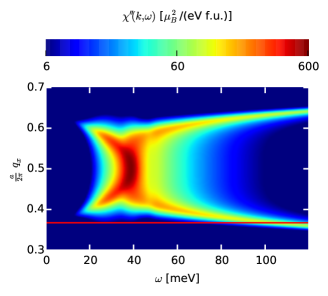
Figure 1: Cut of the spin excitation spectrum $\chi^{\prime\prime}(\boldsymbol{q},\omega)$ along the nodal axis, calculated using the set of parameter values $S_{1}$. The solid red line corresponds to the position of the vector $\boldsymbol{Q}_{0}$ shown in Fig. 2.

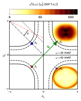
Figure 2: The Fermi surfaces for the antibonding (dashed line), and bonding (solid line) bands, obtained using the set of parameter values $S_{1}$. The solid green arrow represents the interband scattering vector $\boldsymbol{Q_{0}}$. The red dashed-dotted line (the nearby dashed line) indicates an example of the Fermi surface cut used in Subsec. IV.1 ( IV.2). Also shown are two (suitably shifted) constant energy cuts of the spin susceptibility. The one shown in the upper right quadrant corresponds to $\chi^{\prime\prime}(\boldsymbol{k}-\boldsymbol{k}_{A_{1}},\omega=\text{$38\text{\,}\mathrm{meV}$})$, the one shown in the bottom right quadrant to $\chi^{\prime\prime}(\boldsymbol{k}-\boldsymbol{k}_{A_{2}},\omega=\text{$80\text{\,}\mathrm{meV}$})$.

Finally, we address the coupling constant $g$. In Ref. Dahm et al., 2009, the magnitude of the superconducting gap $\Delta_{\text{SC}}$ was fixed ($\Delta_{\text{SC}}=\text{$30\text{\,}\mathrm{meV}$}$), so that the value of the coupling constant $g$ could be obtained by imposing that the value of the calculated renormalized Fermi velocity be consistent with the angle resolved photoemission (ARPES) data. This choice leads to a high value of the superconducting transition temperature $T_{\text{c}}$ of $174\text{\,}\mathrm{K}$. In the present work, the iterative solution of Eqs. (1) and (3) has been performed in a fully self-consistent manner, along the lines of Refs. Chaloupka and Munzar, 2007; Šopík et al., 2015. The renormalized dispersions are adjusted at each iteration, following the approach developed in Refs. Dahm et al., 2009; Dahm and Scalapino, 2013, in such a way that the renormalized Fermi surfaces are fixed and match the ARPES profiles used as inputs. Within this framework, $\Delta_{\text{SC}}$ is not constrained, so that its dependence on $g$ has allowed us to fix the value of $g$ by requiring that $\Delta_{\text{SC}}=\text{$30\text{\,}\mathrm{meV}$}$. The resulting value of $g$ of $1.0\text{\,}\mathrm{eV}$ is considerably smaller than that of Ref. Dahm et al., 2009 (the coupling constant of the latter reference $\bar{U}$ is connected to our $g$ by $\bar{U}=g\sqrt{{2}\over{3}}$, and the value of $\bar{U}$ used therein corresponds to $g=\text{$1.95\text{\,}\mathrm{eV}$}$). The renormalization of the nodal Fermi velocity is weaker and the value of $T_{\text{c}}$ lower with this smaller value of $g$. The set of parameter values just introduced is the main set used throughout the paper, and is referred to as set $S_{1}$.

The calculations have been performed using the fast Fourier transform algorithm, taking full advantage of the symmetries of the system. We have used a grid of $256\times 256$ points in the Brillouin zone and a cutoff of $4\text{\,}\mathrm{eV}$ to limit the number of Matsubara frequencies. We have checked, by varying the density of the grid and the cutoff, that these values are sufficient.

III The kink in the dispersion relation along the nodal axis

III.1 Role of the upper branch of $\chi^{\prime\prime}$

The solid blue line in Fig. 3 represents the electronic dispersion along the nodal axis for the bonding band. For a given energy, the associated value of $k$ is obtained as the root of the real part of the denominator of Eq. (3). It coincides with the value of $k$ corresponding to the maximum of the spectral function for the given energy. The dashed line connects the quasiparticle peak at $k_{F}$ and the maximum of the spectral function corresponding to the high energy cutoff of $250\text{\,}\mathrm{meV}$. The kink is smooth and broad, with a relatively small amplitude. The discrepancy between this profile and the result of Ref. Dahm et al., 2009 is mainly due to the lower value of $g$ used in the present study, as discussed in detail in Subsec. III.2.

The position and the profile of the kink can be understood in terms of a combination of the geometrical features of the Fermi surfaces and those of the spin susceptibility spectrum. Consider a scattering process whereby an electron from the bonding band, of quasimomentum $\boldsymbol{k}$ and energy $E$, is scattered to the antibonding band, quasimomentum $\boldsymbol{k}-\boldsymbol{q}$ and energy $E-\omega$, while a spin excitation of quasimomentum $\boldsymbol{q}$ and energy $\omega$ is emitted (an example with $\boldsymbol{k}=\boldsymbol{k}_{B_{1}}$ and $\boldsymbol{q}=\boldsymbol{Q}_{0}\equiv\boldsymbol{k}_{B_{1}}-\boldsymbol{k}_{A_{1}}$ is shown in Fig. 2). The process can occur with a considerable probability only if the momentum $\boldsymbol{q}$ is such that $\chi^{\prime\prime}(\boldsymbol{q},\omega)$ is significant. Let us consider scattering processes along the direction of the Brillouin zone diagonal, from the region around $\boldsymbol{k}_{B_{1}}$ to the region around $\boldsymbol{k}_{A_{1}}=\boldsymbol{k}_{B_{1}}-\boldsymbol{Q}_{0}$. Figure 2 shows that such processes have a negligible probability for $\omega\simeq\text{$40\text{\,}\mathrm{meV}$}$ (see the constant energy cut shown in the upper right quadrant of Fig. 2). The contribution of the resonance mode to the quasiparticle self-energy $\widehat{\Sigma}^{B}_{|\boldsymbol{k}=\boldsymbol{k}_{B_{1}}}$ can thus be expected to be negligible, and the nodal dispersion to be almost unaffected by the presence of the resonance mode. For $\omega\simeq\text{$80\text{\,}\mathrm{meV}$}$ – the energy of the crossing point of the red line and the upper branch of the hourglass in Fig. 1 –, however, the probability is considerable (see the constant energy cut in the lower right quadrant of Fig. 2). The nodal dispersion can thus be expected to be strongly influenced by the coupling to spin excitations of the upper branch. Indeed, the calculated spectrum of $\operatorname{Im}{\widehat{\Sigma}^{B}_{|\boldsymbol{k}=\boldsymbol{k}_{B_{1}}}}$, shown in Fig. 5, does not exhibit any significant feature around $40\text{\,}\mathrm{meV}$ due to the resonance mode. Instead, it displays a steep onset around $80\text{\,}\mathrm{meV}$ due to the upper branch.

The kink itself (defined as the minimum of the second derivative of the dispersion) is located at a higher energy of about $130\text{\,}\mathrm{meV}$. The difference is due to two facts. (a) The kink energy corresponds to the energy of the maximum of the real part of the self-energy (connected to its imaginary part through the Kramers-Kronig relation). This maximum is located at an energy higher than that of the onset of the imaginary part. This issue is discussed in detail in Subsec. III.2. (b) The self-energy is $k$-dependent and in the region of $k$-space around the kink (where $|\boldsymbol{k}|<k_{F,\,N}^{B}$), its imaginary part sets on at a higher energy than for $k$ close to $k_{F,\,N}^{B}$. This can be inferred from Figure 1: the energy of the crossing point of the upper branch of $\chi^{\prime\prime}$ with a fixed $q$ horizontal line increases when the magnitude of $q$ decreases. The impact of the $k$-dependence of the self-energy on the energy of the kink is quantitatively assessed in Subsec. III.2. The validity of the simple relation between the kink energy and the boson energy has been examined, in a different context, by Schachinger and CarbotteSchachinger and Carbotte (2009).

The above analysis confirms the conclusions of Ref. Dahm et al., 2009 regarding the origin of the kink. However, it additionally reveals that the presence of the upper branch per se is not a sufficient condition for it to play the prominent role in the formation of the nodal kink. Another necessary condition is the simultaneous occurrence of a low kurtosisDeCarlo (1997) of $\chi^{\prime\prime}(\boldsymbol{q},\omega_{\text{res}})$ (where $\omega_{\text{res}}$ is the frequency of the resonance mode) and of a relatively small value of $|\boldsymbol{Q}_{0}|$. Only under these conditions is the contribution of the resonance mode negligible. A higher kurtosis of $\chi^{\prime\prime}(\boldsymbol{q},\omega_{\text{res}})$ or a larger value of $|\boldsymbol{Q}_{0}|$ would allow the contribution of the resonance to be large enough and dominate that of the high-energy branch. This effect was confirmed by separate calculations of the respective contributions of the resonance mode and of the upper branch/continuum for various shapes of the spectrum of $\chi^{\prime\prime}$.

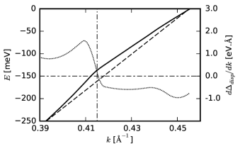
Figure 3: Dispersion relation along the Brillouin zone diagonal for the bonding band. The solid line represents the renormalized dispersion. The dashed line represents a linear approximation to the bare dispersion. The dotted line is the derivative of the difference $\Delta_{\text{disp}}$ between the renormalized dispersion and the bare dispersion. The vertical dash-dotted line is a guide to the eye. The calculations have been performed using the set of parameter values $S_{1}$.

The low kurtosis exhibited by $\chi^{\prime\prime}(\boldsymbol{q},\omega_{\text{res}})$ is illustrated in Fig. 4, which displays $\chi^{\prime\prime}_{\text{int}}(q)=\int_{0}^{\text{$40\text{\,}\mathrm{meV}$}}\chi^{\prime\prime}(q,\omega)d\omega$ as a function of $q$ for $\boldsymbol{q}$ along the Brillouin zone diagonal. The figure allows us to assess the $q$-space distribution of the spectral weight of low energy spin fluctuations including the resonance mode. The solid green line, corresponding to the spectrum of $\chi^{\prime\prime}$ used in the present study, exhibits a broad peak and thin tails, both characteristic of a distribution with low kurtosis. The dashed blue line corresponds to the form of the spin susceptibility used by two of the present authors in previous studiesMunzar et al. (1999); Cásek et al. (2005); Chaloupka and Munzar (2007) (the MBC form in the following). It possesses a higher kurtosis, with both a narrower peak and fatter tails. Finally, the black dash-dotted line represents the susceptibility profile used by Eschrig and Norman in their thorough analysis of the dispersion anomalies within the spin-fermion modelEschrig and Norman (2003) (see also Ref. Eschrig, 2006). It also displays a relatively high kurtosis. The vertical red dashed line sits at the position of the interband vector $\boldsymbol{Q}_{0}$. It can be seen that both for the MBC profile and for the Eschrig-Norman one, $\chi^{\prime\prime}_{\text{int}}(|\boldsymbol{Q}_{0}|)$ is significant, approximately an order of magnitude larger than the corresponding value for the present spectrum of $\chi^{\prime\prime}$. This has a direct impact on the magnitude of the contribution of the resonance mode to the quasiparticle self-energy. Note, that the spectrum of $\chi^{\prime\prime}$ used here was obtained from a fit to experimental inelastic neutron scattering data, while the other two spectra (MBC and Eschrig-Norman) are based on assumptions about the $q$-dependence. The considerations here are complementary to those of a previous work by Chubukov and NormanChubukov and Norman (2004), where the weakening of the effect of the resonance on the near nodal dispersion has been addressed using an analytical approach.

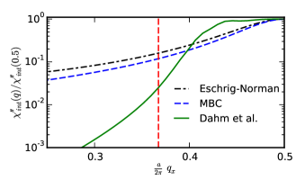
Figure 4: The quantity $\chi^{\prime\prime}_{\text{int}}$, defined in the text, as a function of $q_{x}$ along the Brillouin zone diagonal. The three lines correspond to the three profiles of $\chi^{\prime\prime}(\boldsymbol{q},\omega)$ discussed in the text. The vertical red dashed line indicates the position of the interband vector $\boldsymbol{Q_{0}}$.

III.2 Impact of the magnitude of the coupling constant

In this subsection, we examine the link between the kink in the nodal dispersion and the features of the fermionic self-energy. Using Eq. (3), we find that the renormalized velocity $v$ for a quasimomentum $k$ along the nodal axis is given by:

$$v(\bar{\epsilon}_{k})=\dfrac{v_{0}(\bar{\epsilon}_{k})+\partial_{k}\Sigma^{\prime}(k,\bar{\epsilon}_{k})}{1-\partial_{E}\Sigma^{\prime}(k,\bar{\epsilon}_{k})},$$ (4)

where $v_{0}$ is the bare velocity and $\bar{\epsilon}_{k}$ the renormalized dispersion. The known form of the bare velocity allows one to approximate $v_{0}(\bar{\epsilon}_{k})$ by its value at the Fermi surface, $v_{F_{0}}$. Moreover, it is usually assumed that the momentum dependence of the self-energy is weakEschrig (2006), so that the term $\partial_{k}\Sigma^{\prime}(k,\bar{\epsilon}_{k})$ in Eq. (4) can be neglected, and the term $\partial_{E}\Sigma^{\prime}(k,\bar{\epsilon}_{k})$ replaced with $\partial_{E}\Sigma^{\prime}(k=k_{F},\bar{\epsilon}_{k})$. With these approximations, the energy dependence of $v$ is determined by the renormalization factor $Z(\bar{\epsilon}_{k})=1-\partial_{E}\Sigma^{\prime}(k=k_{F},\bar{\epsilon}_{k})$, and the energy of the kink coincides with the energy of the extremum of $\Sigma^{\prime}(k=k_{F},\bar{\epsilon}_{k})$. In the following, we quantitatively assess the impact of the momentum dependence of the self-energy on the kink energy and shape, and identify two qualitatively distinct regimes.

Figure 5 illustrates the relationship between the energy of the kink and the energies of the features of the self-energy, for the set of parameter values $S_{1}$. It shows the graphical solution of the equation for the quasiparticle energy $\bar{\epsilon}_{k}$, for two values of $k$ along the nodal axis: $k_{F,\,N}^{B}$ and $k_{\text{kink}}$ (the value of quasimomentum at which the kink occurs). Also shown are the corresponding spectra of the real and imaginary components of the normal self-energy, and for $k_{\text{kink}}$, in addition, the normal spectral function $A_{k}(E)$. The spectral function for $k_{F,\,N}^{B}$ possesses a sharp quasiparticle peak at $E=0$. For each of the two values of $k$, $\bar{\epsilon}_{k}$ is determined as the energy of the crossing between the corresponding black line (representing $E-\epsilon_{k}+\mu$) and the corresponding blue line (representing $\operatorname{Re}{\Sigma(k,E)}$). The energies of the crossing points coincide with those of the quasiparticle peaks of $A_{k}(E)$, as expected. It can be seen that $\Sigma^{\prime\prime}_{k=k_{F,\,N}^{B}}$ sets on at around $80\text{\,}\mathrm{meV}$ as discussed in Sec. III.1, and that the maximum of its Kramers-Kronig transform $\Sigma^{\prime}_{k=k_{F,\,N}^{B}}$ occurs at a higher energy (approximately $110\text{\,}\mathrm{meV}$) due to the finite width of the step in $\Sigma^{\prime\prime}_{k=k_{F,\,N}^{B}}$. Finally, the aforementioned assumption of weak momentum dependence of the self-energy can be seen to be valid: even though the energy of the maximum of $\Sigma^{\prime}_{k=k_{\text{kink}}}$ is higher than that of the maximum of $\Sigma^{\prime}_{k=k_{F,\,N}^{B}}$ by $\Delta_{\text{kink}}\simeq\text{$20\text{\,}\mathrm{meV}$}$, the shapes of the profiles are qualitatively very similar. In particular, a sharp maximum is present in both profiles. This explains why the energy of the kink is only slightly (by $\Delta_{\text{kink}}$) higher than that of the maximum of $\Sigma^{\prime}_{k=k_{F,\,N}^{B}}$, and why the kink is relatively sharp.

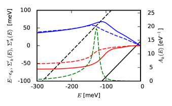
Figure 5: Graphical solution of the equation for the quasiparticle energy $\bar{\epsilon}_{k}$, for two different values of $k$ along the nodal axis: $k=k_{F,\,N}^{B}$ and $k_{\text{kink}}$ (i.e., the value of quasimomentum for which the nodal kink occurs), and the corresponding spectra of the real and imaginary parts of the self-energy, and of the spectral function $A_{k}(E)$. The calculations have been performed using the set of parameter values $S_{1}$. The solid lines correspond to $k=k_{F,\,N}^{B}$, the dashed lines to $k=k_{\text{kink}}$. The black lines represent the linear functions $E-\epsilon_{k}-\mu$, the red lines the imaginary parts of the self-energy, whose real parts are shown in blue. The green line represents the spectral function for $k_{\text{kink}}$.

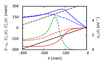
Figure 6: The same quantities as in Fig. 5, calculated with the same input parameter values, except for $g=\text{$1.95\text{\,}\mathrm{eV}$}$, consistent with Ref. Dahm et al., 2009. Notice the change in the scale of the left axis, compared with Fig. 5.

It is worth contrasting these findings with the results of the fully self-consistent approach with the value of the coupling constant $g$ of $1.95\text{\,}\mathrm{eV}$ (as in Ref. Dahm et al., 2009) in place of $g=\text{$1.0\text{\,}\mathrm{eV}$}$. Figure 6 illustrates the properties of the system in this case. The large value of the coupling constant induces much larger magnitudes of the real and imaginary parts of the self-energy than in the former case. Thus, the maximum value of $\Sigma^{\prime}_{k=k_{F,\,N}^{B}}$ is much larger, and the distance between $k_{F,\,N}^{B}$ and $k_{\text{kink}}$ as well. Figure 6 shows that over such a broad $k$-interval, the quasimomentum dependence of $\Sigma^{\prime}(k,E)$ may no longer be considered to be weak. The flattening of $\Sigma^{\prime}$ as $k$ moves away from the Fermi surface (expected irrespective of the chosen set of parameter values) is large enough for the profile to change qualitatively. In particular, the pronounced maximum of $\Sigma^{\prime}$ disappears before the $E-\epsilon_{k}+\mu$ line reaches it. Therefore, the position and the shape of this extremum at $k_{F,\,N}^{B}$ are not the critical factors determining the energy and the shape of the kink anymore. Instead, the dependence of the self-energy on $k$ has a substantial impact on the profile of the kink. In terms related to Eq. (4), this means that the weak momentum approximation breaks down.

The interpretation of the formation of the kink therefore differs qualitatively between the former and the latter case. In the low-$g$ regime, the energy of the kink is approximately given by the energy of the maximum of $\Sigma^{\prime}(k_{F,\,N}^{B},\bar{\epsilon}_{k})$, and the kink is sharp. In the high-$g$ regime, the kink is made smoother by the influence of the momentum dependence of $\Sigma^{\prime}$.

IV The kink in the dispersion relation away from the nodal axis

Having analyzed the behavior of the kink in the dispersion relation along the Brillouin zone diagonal, we now proceed to examine how the situation evolves away from the nodal axis, as a function of the angle $\theta$ between the direction of the Fermi surface cut and the diagonal (for a definition of $\theta$, see Fig. 2).

IV.1 Effective self-energy approach

First, we follow the approach introduced by Plumb et al. Plumb et al. (2013). Figure 7 shows a heat map of $\operatorname{Re}{\Sigma_{\text{eff}}(\theta,E)}$, the real part of the effective self-energy defined by Eq. (1) of Ref. Plumb et al., 2013, and used in order to track the angular dependence of the kinkPlumb et al. (2013). For the convenience of the reader, the definition of $\Sigma_{\text{eff}}(\theta,E)$ will be restated here. Denote the inverse of the renormalized dispersion relation for a given value of $\theta$ by $\bar{k}(\theta,E)$. Then we define $\operatorname{Re}{\Sigma_{\text{eff}}(\theta,E)}\equiv\bar{\epsilon}_{k=\bar{k}(\theta,E)}-\epsilon_{k=\bar{k}(\theta,E)}$. In the present work, we have followed the approach of Ref. Plumb et al., 2013, and approximated the bare dispersion by a straight line connecting the quasiparticle peak at $k_{F}$ and the maximum of the spectral function corresponding to the high energy cutoff of $200\text{\,}\mathrm{meV}$. The heat map has been obtained by an interpolation of the results for a discrete set of $\theta$-values. For each of these values, the red circle indicates the energy of the maximum of $\operatorname{Re}{\Sigma_{\text{eff}}}$, coinciding with the energy $\Omega_{\text{kink}}(\theta)$ of the kink in the fermionic dispersion.

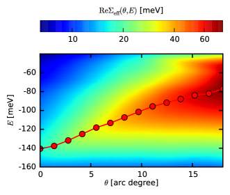
Figure 7: Heat map of the real part of the effective self-energy $\Sigma_{\text{eff}}(\theta,E)$ defined in the text, calculated using the set of parameter values $S_{1}$. For each of the selected values of $\theta$, the red circle represents the energy of the maximum of $\operatorname{Re}{\Sigma_{\text{eff}}(\theta,E)}$, which coincides with the energy of the kink.

The most striking aspect of the result is the strong angular dependence of $\Omega_{\text{kink}}$. With increasing $\theta$, $\Omega_{\text{kink}}$ decreases and the intensity and the sharpness of the kink increase. Both observations are in qualitative agreement with the experimental findings of Ref. Plumb et al., 2013. These trends can be understood in terms of the interplay between the fermionic dispersion and the bosonic spectrum, discussed for the case of $\theta=\text{$$}$ in Sec. III.1. As the Fermi surface cut moves away from the nodal axis, the modulus of the interband scattering vector along the $(\pi/a,\pi/a)$ direction increases. As a consequence, the section of $\chi^{\prime\prime}$ which contributes most to the scattering, changes. As Fig. 1 shows, the spectral weight of the constant-$q$ cut of the upper branch of $\chi^{\prime\prime}$ increases, and the energy of the maximum decreases as $q$ increases towards $0.5$ from below. The profile of the self-energy can be expected to follow the same trend, which indeed occurs in Fig. 7.

Following this analysis, we are in a position to conjecture that for large values of $\theta$, the contribution of the resonance mode to the scattering becomes large, and eventually dominates the profile. This should be accompanied by a change of sign of the slope of $\Omega_{\text{kink}}(\theta)$ at a critical angle $\theta_{c}$. Simple geometrical considerations based on Fig. 2 provide $\theta_{c}\simeq\text{$$}$. The coupling to the resonance mode has been put forward as the source of the dispersion anomalies in earlier spin-fermion model based studiesEschrig (2006); Eschrig and Norman (2003). Within the framework of these studies, however, the scattering mechanism does not exhibit a very strong angular dependence, given the high kurtosis of the resonance mode. A more precise analysis of the situation, presented in Sec. IV.2, shows that $\theta_{c}$ is larger than $20\mathrm{°}$, and that for $\theta>\theta_{c}$, the effective self-energy approach introduced above does not provide reliable estimates of the kink energy.

Note finally that the scenario outlined above is – from the qualitative point of view – analogous to the one proposed by Hong and ChoiHong and Choi (2013). These authors have also argued that the observed complex structure of the quasiparticle self-energy and its evolution when going from the nodal cut to the antinodal one is determined by the presence of two independent contributions: that of a resonance mode and the one of a separate branch of bosonic excitations.

IV.2 Relation between the kink and the features of the quasiparticle self-energy

Here we present a different approach to determine the angular dependence of the kink energy, based on a numerical procedure for estimating the roots of the real part of the denominator of the Green’s function (3). This method is particularly well suited to the study of the kink for larger values of $\theta$. For numerical reasons we use here slightly different Fermi surface cuts than in Subsec.IV.1. The present ones are parallel to the Brillouin zone diagonals. For an example of the two types of cuts, see Fig. 2.

The $2\times 2$ self-energy matrix can be expressed in terms of the Pauli matrices:

$$\widehat{\Sigma}(\boldsymbol{k},E)\equiv\Sigma_{0}(\boldsymbol{k},E)\hat{\tau_{0}}+\xi(\boldsymbol{k},E)\hat{\tau_{3}}+\phi(\boldsymbol{k},E)\hat{\tau_{1}},$$

and the Nambu propagator as

$$\widehat{G}(\boldsymbol{k},E)=\biggl{[}\widehat{G}_{0}^{-1}(\boldsymbol{k},E)-\widehat{\Sigma}(\boldsymbol{k},E)\biggr{]}^{-1}$$

$$= \dfrac{\bigl{[}E-\Sigma_{0}(\boldsymbol{k},E)\bigr{]}\hat{\tau_{0}}+\widetilde{\epsilon}(\boldsymbol{k},E)\hat{\tau_{3}}+\phi(\boldsymbol{k},E)\hat{\tau_{1}}}{\bigl{[}E-\Sigma_{0}(\boldsymbol{k},E)\bigr{]}^{2}-\widetilde{\epsilon}(\boldsymbol{k},E)^{2}-\phi(\boldsymbol{k},E)^{2}}.$$

We have dropped the band index for simplicity, and $\widetilde{\epsilon}(\boldsymbol{k},E)$ stands for $\epsilon(\boldsymbol{k},E)-\mu+\xi(\boldsymbol{k},E)$. The normal component of the propagator is given by

$$G(\boldsymbol{k},E)=\dfrac{E-\Sigma_{0}(\boldsymbol{k},E)+\widetilde{\epsilon}(\boldsymbol{k},E)}{\bigl{[}E-\Sigma_{0}(\boldsymbol{k},E)\bigr{]}^{2}-\widetilde{\epsilon}(\boldsymbol{k},E)^{2}-\phi(\boldsymbol{k},E)^{2}}.$$ (5)

The approach we introduce here is most easily pictured as an extension of Sec. III.2 and Fig. 5 to the case where $\phi(\boldsymbol{k},E)$ is finite. Provided the quasiparticle is well defined, its energy $E$ is equal to the root of the real part of the denominator, i.e., to the solution of the following equation in $E$, parametrized by $\boldsymbol{k}$:

$$\operatorname{Re}{\left[\left(E-S(\boldsymbol{k},E)\right)\left(E-D(\boldsymbol{k},E)\right)-\widetilde{\epsilon}(\boldsymbol{k},E)^{2}\right]}=0,$$ (6)

where $S(\boldsymbol{k},E)\equiv\Sigma_{0}(\boldsymbol{k},E)\pm\phi(\boldsymbol{k},E)$ and $D(\boldsymbol{k},E)\equiv\Sigma_{0}(\boldsymbol{k},E)\mp\phi(\boldsymbol{k},E)$. The upper (lower) sign is used if $\operatorname{Re}{\Sigma_{0}(\boldsymbol{k},E)}$ and $\operatorname{Re}{\phi(\boldsymbol{k},E)}$ have the same (opposite) signs (recall that $\operatorname{Re}{\phi(\boldsymbol{k},E)}$ possesses d-wave symmetry, while $\operatorname{Re}{\Sigma_{0}(\boldsymbol{k},E)}$ is positive in the momentum-energy section we are considering). Assuming that the imaginary parts of $E-S(\boldsymbol{k},E)$ and $E-D(\boldsymbol{k},E)$ are small compared to their real parts, we may approximate Eq.(6) by:

$$\operatorname{Re}{\left[\left(E-S(\boldsymbol{k},E)\right)\right]}\simeq\dfrac{\operatorname{Re}{\left[\widetilde{\epsilon}(\boldsymbol{k},E)^{2}\right]}}{\operatorname{Re}{\left[\left(E-D(\boldsymbol{k},E)\right)\right]}}.$$ (7)

The validity of this assumption is related to that of the quasiparticle picture, for an illustration, see Fig. 8.

For $\theta=\text{$$}$, $S(\boldsymbol{k},E)=D(\boldsymbol{k},E)=\Sigma_{0}(\boldsymbol{k},E)$ and Eq. (7) reduces to the simple equation determining the quasiparticle energy employed in Sec. III, $\operatorname{Re}{\left[E-\Sigma_{0}(\boldsymbol{k},E)-\widetilde{\epsilon}(\boldsymbol{k},E)\right]}=0$.

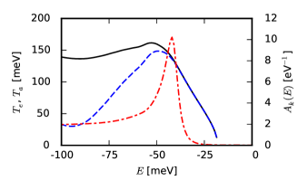
Figure 8: Comparison of the expression from Eq. (6), $T_{\text{e}}\equiv\bigl{(}\operatorname{Re}{\left[\left(E-S(\boldsymbol{k},E)\right)\left(E-D(\boldsymbol{k},E)\right)\right]}\bigr{)}^{1/2}$ (black solid line) with its approximation $T_{\text{a}}\equiv\bigl{(}\operatorname{Re}{\left[E-S(\boldsymbol{k},E)\right]}\operatorname{Re}{\left[E-D(\boldsymbol{k},E)\right]}\bigr{)}^{1/2}$ used in Eq. (7) (dashed blue line), for $k=k_{\text{kink}}$ corresponding to the cut defined by $\theta=\text{$$}$. The dashed-dotted line represents the spectral function $A_{k}(E)$. The calculations have been performed using the set of parameter values $S_{1}$.

For large values of $\theta$, where the gap is fully developed, $\Sigma_{0}(\boldsymbol{k},E)$ and $\phi(\boldsymbol{k},E)$ have comparable magnitudes. As a consequence, $\operatorname{Re}{\left[E-S(\boldsymbol{k},E)\right]}$ and $\operatorname{Re}{\left[E-D(\boldsymbol{k},E)\right]}$ exhibit very different profiles, while both remain weakly $k$-dependent along a fixed cut. This is illustrated by Fig. 9, which shows the approximately linear profile of $\operatorname{Re}{\left[E-D(k,E)\right]}_{|\theta=\text{$$}}$, contrasting with the peaked shape of $\operatorname{Re}{\left[E-S(k,E)\right]}_{|\theta=\text{$$}}$. The former profile, close to linear, emerges as the difference between two similarly peaked functions $\Sigma_{0}(\boldsymbol{k},E)$ and $\phi(\boldsymbol{k},E)$ (plus the linear function $E$). The similarity is due to the fact that both functions result from the convolution in Eq. (2). The latter profile represents the sum of the two functions (plus the linear function $E$), and therefore exhibits a peaked shape reminiscent of the similar shape of both functions.

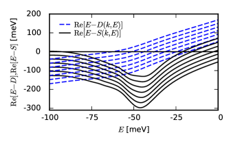
Figure 9: Profiles of the terms $\operatorname{Re}{\left[E-D(k,E)\right]}$ and $\operatorname{Re}{\left[E-S(k,E)\right]}$ entering Eq. (7), for $\theta=\text{$$}$ and for a set of values of the quasimomentum $k$, calculated using the set of parameter values $S_{1}$. The lowest curves correspond to the Fermi surface. The quasimomentum $k$ differs by $\Delta k=\pi/128$ from one curve to the next. For readability, each curve is shifted by $20\text{\,}\mathrm{meV}$ with respect to the previous one as $k$ moves away from the Fermi surface.

The expressions entering Eq. (7) can be interpreted in simple terms. The one on the left hand side displays a peak whose magnitude increases with increasing $\theta$ as a consequence of the lengthening of the interband scattering vector, and of the corresponding increase of the spectral weight of the section of $\chi^{\prime\prime}$ which contributes to the scattering processes. The term on the right-hand side of Eq. (7) involves the inverse of an approximately linear expression. For fixed values of $\theta$ and $\boldsymbol{k}$, the value of this expression at the origin equals $|\operatorname{Re}{\phi(\boldsymbol{k},E=0)}|$. These observations allow us to interpret the profile of the right-hand side of Eq. (7) as that of a hyperbola-like function, with the origin of the $E$-axis displaced by $-|\operatorname{Re}{\phi(\boldsymbol{k},E=0)}|\simeq-|\operatorname{Re}{\phi(\boldsymbol{k}=\boldsymbol{k}_{F}(\theta),E=0)|}=\Delta_{\text{SC}}(\theta)$, as illustrated in Fig. 10. As $\boldsymbol{k}$ moves away from the Fermi surface, a family of hyperbola-like functions (“hyperbolas” in the following) is generated, with a multiplicative factor $\operatorname{Re}{\left[\widetilde{\epsilon}(\boldsymbol{k},E)^{2}\right]}$ applied to the $y$-axis. The right-hand side of Eq. (7) thus evolves from a very sharp hyperbola, for $k\to k_{F}(\theta)$ , to a smooth hyperbola, for large values of $|k-k_{F}(\theta)|$.

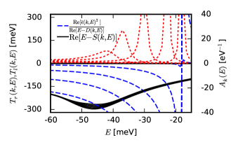
Figure 10: Profiles of both sides of Eq. (7) and of the quasiparticle spectral function $A_{k}(E)$ for $\theta=\text{$$}$ and for a set of values of the quasimomentum $k$, calculated using the set of parameter values $S_{1}$. As in Fig. 9, the quasimomentum $k$ differs by $\Delta k=\pi/128$ from one curve to the next. The set of dashed blue (solid black) lines represents the term $T_{r}(\boldsymbol{k},E)\equiv\operatorname{Re}{\left[\widetilde{\epsilon}(\boldsymbol{k},E)^{2}\right]}/\operatorname{Re}{\left[\left(E-D(\boldsymbol{k},E)\right)\right]}$ (the term $T_{l}(\boldsymbol{k},E)\equiv\operatorname{Re}{\left[\left(E-S(\boldsymbol{k},E)\right)\right]}$). Note that the energies of the peaks of the spectral function (dotted red line) coincide with those of the crossing points of the corresponding blue and black lines.

This analysis shows that the left-hand (right-hand) side term of Eq. (7), indexed by $(k,\theta)$, is strongly (weakly) dependent on $\theta$, but weakly (strongly) dependent on $k$. In other words, Eq. (7) allows us to disentangle the sensitivities of the quantities of interest with respect to $k$ and $\theta$. At this point, noticing that neither $\operatorname{Re}{\widetilde{\epsilon}(\boldsymbol{k},E)}$ nor $D(\boldsymbol{k},E)$ exhibit a pronounced kink, we are in a position to conclude that the origin of the kink in the fermionic dispersion lies in the kink exhibited by the left hand side of Eq. 7, $\operatorname{Re}{\left[\left(E-S(\boldsymbol{k},E)\right)\right]}$. The position of the kink can now be reliably evaluated by exploring the smooth quantity $\operatorname{Re}{\left[\left(E-S(\boldsymbol{k},E)\right)\right]}$ defined on the fine energy mesh.

The approach detailed below has been used to obtain the profile of $\Omega_{\text{kink}}(\theta)$ displayed in Fig. 11: For each selected value of $\theta$, the momentum dependence of the self-energy is examined. We then define $k_{0}(\theta)$ as the value of $k$ on the computational $k$-mesh, along the considered $\theta$-cut (recall that the $k$-space cuts we use in this subsection have the advantage of matching the geometry of the computational $k$-mesh), which is closest to $k_{\text{kink}}(\theta)$. This process is illustrated in Fig. 10. Given a value of $\theta$, $k_{0}(\theta)$ is the value of $k$, such that the dashed line representing $\operatorname{Re}{\left[\widetilde{\epsilon}(\boldsymbol{k},E)^{2}\right]}/\operatorname{Re}{\left[\left(E-D(\boldsymbol{k},E)\right)\right]}$ crosses the solid line representing $\operatorname{Re}{\left[\left(E-S(\boldsymbol{k},E)\right)\right]}$ close to its extremum. Once $k_{0}$ is fixed, we obtain the energy of the kink as that of the extremum of $\operatorname{Re}{S(\boldsymbol{k}_{0},E)}$ (we have checked that in the present context the two energies coincide). As discussed above, in the $\theta\to 0$ limit, this method for estimating the energy of the kink is equivalent to the one used in Sec. III.2 , but there is one caveat: for small values of $\theta$, the gap is small, so that the kink in $E-S(\boldsymbol{k},E)$ is weak and may not always dominate the very weak kink in $E-D(\boldsymbol{k},E)$. As a consequence, for small values of $\theta$, the former method may be more accurate in estimating the energy of the kink.

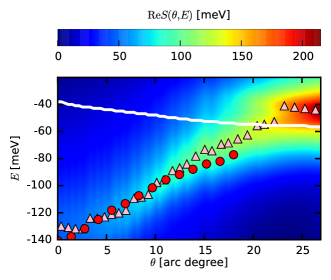
Figure 11: Heat map of the real part of the quantity $S(\boldsymbol{k},E)$ defined in the text, calculated using the set of parameter values $S_{1}$. For each of the selected values of $\theta$, the pink triangle represents the energy of the extremum of $\operatorname{Re}{S(\boldsymbol{k},E)}$, which coincides with $\Omega_{\text{kink}}$, as discussed in the text. The solid white line represents the expression $\omega_{\text{res}}+\Delta_{\text{SC}}(\theta)$. The solid red circles, displayed for comparison, are taken from Fig. 7.

It can be seen in Fig. 11 that the present $\Omega_{\text{kink}}(\theta)$ is close to the result shown in Sec. IV.1. The main discrepancies appear in the $\theta\to 0$ region (discussed above), and for large values of $\theta$. The latter arise because the kink becomes so intense, and sharp in momentum space, that the former method, based on interpolations of the renormalized dispersion in $k$-space, does not provide a precise estimate of the kink energy.

The increased extent of the accessible $\theta$-domain allows for a confirmation of the conjecture exposed in Sec. IV.1, related to the role of the resonance mode. Figure 11 clearly shows that the slope of $\Omega_{\text{kink}}(\theta)$ changes sign at $\theta_{c}\simeq\text{$$}$. We argued in Sec. IV.1 that if the kink is due to the upper branch of $\chi^{\prime\prime}$, then the slope of $\Omega_{\text{kink}}(\theta)$ must be negative. This is the trend observed for $\theta<\theta_{c}$. Conversely, if the resonance mode is the dominant source of scattering, the $\theta$-dependence of $\Omega_{\text{kink}}(\theta)$ is determined mainly by that of $\Delta_{\text{SC}}(\theta)$ and $\Omega_{\text{kink}}(\theta)$ must therefore display a positive slope close to that of $\Delta_{\text{SC}}(\theta)$. This is what we observe in the $\theta>\theta_{c}$ region of Fig. 11, where the profile of $\Omega_{\text{kink}}(\theta)$ follows that of $\omega_{\text{res}}+\Delta_{\text{SC}}(\theta)$, represented by the solid white line. The fact that the $\Omega_{\text{kink}}(\theta)$ line is located somewhat above the $\omega_{\text{res}}+\Delta_{\text{SC}}(\theta)$ line is likely due to the influence of the lower branch of $\chi^{\prime\prime}$. The discontinuity of $\Omega_{\text{kink}}(\theta)$ at $\theta=\theta_{c}$ is an artifact related to the method for the numerical determination of $\Omega_{\text{kink}}(\theta)$.

Finally, we note the remarkable similarity between the background of the heat map shown in Fig. 11 and the profile of the upper branch of $\chi^{\prime\prime}$ displayed in Fig. 1, arising from the selfenergy-$\chi^{\prime\prime}$ relation (1). It illustrates the major role played by the upper branch of $\chi^{\prime\prime}$ in the formation of the angular dependence of $\Omega_{\text{kink}}(\theta)$ in the near nodal region.

V Comparison with experimental data

The main trend of Subsection IV.1, i.e. the decrease of $|\Omega_{\text{kink}}|$ when going from the nodal cut to the antinodal one, is consistent with the experimental findings of Ref. Plumb et al., 2013. Our results provide support for the conjecture that the decrease is associated with the dispersion of the upper branch of the hourglass. The calculated value of the energy of the nodal kink ($\simeq$ $130\text{\,}\mathrm{meV}$), however, is much higher than that of underdoped YBCO reported in Ref. Dahm et al., 2009 ($80\text{\,}\mathrm{meV}$). In addition, the calculated magnitude of the slope of $\Omega_{\text{kink}}(\theta)$ ($3.5\text{\,}\mathrm{meV}$ per arc degree) is much higher than the experimental value of Bi2212 reported in Ref. Plumb et al., 2013 ($0.8\text{\,}\mathrm{meV}$ per arc degree). Finally, the renormalized Fermi velocity of $2.8\text{\,}\mathrm{eV}\AA$ on the nodal axis (see Fig. 3), is much larger than the experimental value of underdoped YBCO of $1.8\text{\,}\mathrm{eV}\AA$. This discrepancy is connected with the fact that the value of $g$ used in the set $S_{1}$ is much smaller than that of Ref. Dahm et al., 2009.

Based on our interpretation of the origin of the kink, it is possible to understand the influence of the model parameters on the profile of $\Omega_{\text{kink}}(\theta)$. We are also well equipped to find out which adjustments are necessary in order to reconcile the results of the calculations with the experimental data. It can be expected that $\Omega_{\text{kink}}(\theta=0)$ decreases with increasing interband distance $|\boldsymbol{Q}_{0}|$ (see Fig. 2 for a definition), but that it is not very sensitive to the doping level or the bonding-antibonding splitting (provided that $|\boldsymbol{Q}_{0}|$ and the Fermi velocity are kept fixed). Our analysis also indicates that a widening of the upper branch of the hourglass should lead to a shift of $\Omega_{\text{kink}}(\theta=0)$ towards lower energies and to a reduction of the slope of $\Omega_{\text{kink}}(\theta)$. Finally, reducing the bandwidth of the bare dispersion should induce a lowering of the renormalized Fermi velocity. We have checked these trends by performing calculations of the same type as described in sections III and IV for many different sets of values of the input parameters.

As an example, and an illustration of the sensitivity of the results of the calculations to the input parameter values, we present below results of our calculations obtained using a set of parameter values ($S_{2}$ in the following), where some of the values have been modified along the lines of the previous paragraph. The values of $k_{F,\,N}^{A}$ and $k_{F,\,N}^{B}$ are increased to $36.0\%$ and $40.7\%$ of $\pi\sqrt{2}/a$, respectivelyEmp . This shift applied to the band structure leaves the system well within the limits given by published experimental values: the values of $k_{F,\,N}^{A}$ and $k_{F,\,N}^{B}$ remain smaller than 41%, the common value of the two parameters reported in Ref. Fournier et al., 2010. Furthermore, the corresponding increase in the magnitude of $|\boldsymbol{Q}_{0}|$ is small, so that the resonance mode does not participate in the scattering along the nodal cut, and the qualitative features of Fig. 2 are conserved. The bandwidth of the bare dispersion is reduced by 40%, so that the value of the renormalized Fermi velocity is close to the experimental one, and we set $g=\text{$0.8\text{\,}\mathrm{eV}$}$, so that the maximum value of the gap remains unchanged at $30\text{\,}\mathrm{meV}$. Finally, the upper branch of $\chi^{\prime\prime}$ is made wider, so as to further reduce the value of $\Omega_{\text{kink}}(\theta=0)$ and the slope of the profile of $\Omega_{\text{kink}}$Emp (nged).

Figure 12 displays the renormalized dispersion calculated using the set of parameter values $S_{2}$. It can be seen that the kink is much more pronounced. As expected, the energy of the kink (ca $90\text{\,}\mathrm{meV}$) and the renormalized Fermi velocity (ca $1.5\text{\,}\mathrm{eV}\AA$) are considerably lower than in Fig. 3, and close to the experimental values of Ref. Dahm et al., 2009.

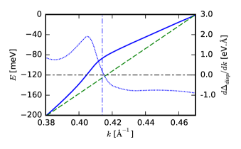
Figure 12: The same quantities as in Fig. 3. The calculations have been performed using the set of parameter values $S_{2}$.

The corresponding angular dependence of $\Omega_{\text{kink}}$ is shown in Fig. 13. It can be seen that the magnitude of the slope of $\Omega_{\text{kink}}$ is reduced to only $1.1\text{\,}\mathrm{meV}$ per arc degree, reasonably close to the experimental value for Bi2212Plumb et al. (2013). The value of $\theta_{c}$ of Fig. 13 (ca $26\mathrm{°}$) is higher than that of Fig. 11. The difference is mainly due to that between the bare dispersion relations of $S_{1}$ and those of $S_{2}$. The interpretation exposed at the end of Sec. IV still applies. Based on this interpretation and the above discussion we can make a prediction concerning the angular dependence of $\Omega_{\text{kink}}$ in underdoped YBCO. We predict that there exists a critical value $\theta_{c}$, such that for $\theta<\theta_{c}$ ($\theta>\theta_{c}$), $\Omega_{\text{kink}}(\theta)$ is a decreasing (weakly increasing) function. The minimum $\Omega_{\text{kink}}(\theta_{c})$ of $\Omega_{\text{kink}}$ is determined by $\Delta_{\text{SC}}(\theta_{c})$ and by the lower branch of $\chi^{\prime\prime}$. A value in the range from $40\text{\,}\mathrm{meV}$ to $60\text{\,}\mathrm{meV}$ can be expected. This prediction could be tested in ARPES experiments.

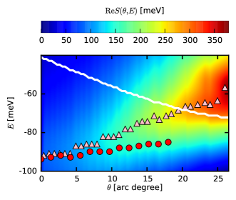
Figure 13: The same quantities as in Fig. 11, calculated using the set of input parameter values $S_{2}$. The apparent steps in the pink triangle profile are due to the reduced energy range of the $E$-axis, and the discretization of the energy mesh.

Finally we address, in light of our findings, the $\Omega_{\text{kink}}(\theta)$ line for nearly optimally doped Bi2212 reported in Ref. Plumb et al., 2013, which was one of our starting points. The energy of the nodal kink in Bi2212 of ca $65\text{\,}\mathrm{meV}$ is roughly $15\text{\,}\mathrm{meV}$ lower than that of underdoped YBCO and $25\text{\,}\mathrm{meV}$ lower than our result shown in Fig. 13. The magnitude of the slope of $\Omega_{\text{kink}}$ in Bi2212 is only slightly smaller than that of our calculations. The difference may be caused by a difference in the Fermi surfaces and/or by a difference in $\chi^{\prime\prime}$. Since the magnitude of the internodal distance, $|\boldsymbol{Q}_{0}|$, of optimally doped Bi2212 is almost the same as that of underdoped YBCO, it appears that some difference in $\chi^{\prime\prime}$ plays the crucial role. Note that the neutron scattering data of optimally doped Bi2212Xu et al. (2009) reveal a fairly high kurtosis of $\chi^{\prime\prime}(q,E)_{|E=\text{$42\text{\,}\mathrm{meV}$}}$ [see Fig. 2 (c) of Ref. Xu et al., 2009], and that the higher energy cuts of $\chi^{\prime\prime}(q,E)$ shown in Figs. 2(a) and 2(b) of Ref. Xu et al., 2009 are considerably wider than those of underdoped YBCO. In particular, the values of $\chi^{\prime\prime}$ for $q=0.19$ r.l.u. (corresponding to $|\boldsymbol{Q}_{0}|$ of Fig. 1) and $\omega=\text{$42\text{\,}\mathrm{meV}$}$, $54\text{\,}\mathrm{meV}$ and $66\text{\,}\mathrm{meV}$ in Figs. 2 (c), (b) and (a) of Ref. Xu et al., 2009, are all significant, and of a comparable magnitude. Motivated by this observation and by the large width of the nodal kink in Bi2212 (see Fig. 1 (d) of Ref. Plumb et al., 2013), we propose the following qualitative interpretation of the angular dependence of $\Omega_{\text{kink}}$ in Bi2212: we suggest that the nodal kink is not determined by a single narrow cut through the upper branch of the hourglass, as in the case of underdoped Y-123 (see Fig. 1), but rather by a broad band of $\chi^{\prime\prime}$ ranging from ca $40\text{\,}\mathrm{meV}$ to ca $100\text{\,}\mathrm{meV}$. Even the $42\text{\,}\mathrm{meV}$ cut contributes because of the high kurtosis. With increasing $\theta$, lower energy segments of $\chi^{\prime\prime}$ become more influential, for the same reasons as discussed in Sec. IV.1, and as a consequence, the energy of the kink slighly decreases.

VI Summary and conclusions

We have investigated the effect of the upper branch of the hour-glass magnetic spectrum on the electronic dispersion of high-T${}_{\text{c}}$ cuprate superconductors using the fully self-consistent version of the phenomenological model, where charged planar quasiparticles are coupled to spin fluctuations. The same input band structure and the same input spin susceptibility as in the previous study by T. Dahm and coworkers have been used.

First, we have confirmed the finding by Dahm et al., that the nodal kink is determined, for the present values of the input parameters, by the upper branch of $\chi^{\prime\prime}$. We have further demonstrated that the position and the shape of the kink depend strongly on the strength of the charge-spin coupling. For low (but still realistic) values of the coupling constant, the position of the kink can be estimated using the common approximation, where the quasimomentum dependence of the self-energy along the Fermi surface cut is neglected. The kink is weak but sharp. For high values of the coupling constant, however, the dependence of the self-energy on the quasimomentum plays an important role. The kink is less sharp, but has a larger amplitude.

Second, we have shown that the kurtosis of the resonance mode of the spin susceptibility in the quasimomentum space has a major influence on the mechanism of the fermionic scattering. If the kurtosis is low (high), as in the present study (as in several previous studiesMunzar et al. (1999); Eschrig and Norman (2003); Cásek et al. (2005); Chaloupka and Munzar (2007)), the effect of the resonance mode in the near-nodal region of the Brillouin zone is weak (large), and the upper branch of the hour-glass (the resonance mode) plays the major role in the formation of the nodal kink.

Third, the calculated energy of the kink decreases as a function of the angle $\theta$ between the Fermi surface cut and the nodal direction. This result is in qualitative agreement with recent experimental resultsPlumb et al. (2013); He et al. (2013). Based on our interpretation of the formation of the kink, we have been able to modify the values of the input parameters in such a way that both the renormalized (nodal) Fermi velocity and the energy of the nodal kink are close to the experimental values for underdoped YBCO reported by Dahm and coworkers. The calculated magnitude of the slope of the angular dependence of the kink energy is close to that of Bi2212 reported by Plumb and coworkers. We predict that there exists a critical value $\theta_{c}$ such that the energy of the kink is a decreasing (weakly increasing) function of $\theta$ for $\theta<\theta_{c}$ ($\theta>\theta_{c}$) and provide a possible qualitative interpretation of the difference between the kink in underdoped YBCO and that in optimally doped Bi2212.

References

- Valla et al. (1999) T. Valla, A. V. Fedorov, P. D. Johnson, B. O. Wells, S. L. Hulbert, Q. Li, G. D. Gu, and N. Koshizuka, Science 285, 2110 (1999).
- Bogdanov et al. (2000) P. V. Bogdanov, A. Lanzara, S. A. Kellar, X. J. Zhou, E. D. Lu, W. Zheng, G. D. Gu, K. Kishio, J. I. Shimoyama, Z. Hussain, et al., Phys. Rev. Lett. 85, 2581 (2000).
- Kaminski et al. (2001) A. Kaminski, M. Randeria, J. C. Campuzano, M. R. Norman, H. Fretwell, J. Mesot, T. Sato, T. Takahashi, and K. Kadowaki, Phys. Rev. Lett. 86, 1070 (2001).
- Lanzara et al. (2001) For a review, see A. Lanzara, P. V. Bogdanov, X. J. Zhou, S. A. Kellar, D. L. Feng, and H. Eisaki, Nature 412, 510 (2001).
- Gromko et al. (2003) A. D. Gromko, A. V. Fedorov, Y.-D. Chuang, J. D. Koralek, Y. Aiura, Y. Yamaguchi, K. Oka, Y. Ando, and D. S. Dessau, Phys. Rev. B 68, 174520 (2003).
- Sato et al. (2003) T. Sato, H. Matsui, T. Takahashi, H. Ding, H.-B. Yang, S.-C. Wang, T. Fujii, T. Watanabe, A. Matsuda, T. Terashima, et al., Phys. Rev. Lett. 91, 157003 (2003).
- Zhang et al. (2008) W. Zhang, G. Liu, L. Zhao, H. Liu, J. Meng, X. Dong, W. Lu, J. S. Wen, Z. J. Xu, G. D. Gu, et al., Phys. Rev. Lett. 100, 107002 (2008).
- Damascelli et al. (2003) For a review of the early results, see A. Damascelli, Z. Hussain, and Z. X. Shen, Rev. Mod. Phys. 75, 473 (2003).
- Devereaux et al. (2004) T. P. Devereaux, T. Cuk, Z. X. Shen, and N. Nagaosa, Phys. Rev. Lett. 93, 117004 (2004).
- Cuk et al. (2004) T. Cuk, F. Baumberger, D. H. Lu, N. Ingle, X. J. Zhou, H. Eisaki, N. Kaneko, Z. Hussain, T. P. Devereaux, N. Nagaosa, et al., Phys. Rev. Lett. 93, 117003 (2004).
- Anderson (2007) P. W. Anderson, Science 316, 1705 (2007).
- Byczuk et al. (2007) K. Byczuk, M. Kollar, K. Held, Y.-F. Yang, I. A. Nekrasov, T. Pruschke, and D. Vollhardt, Nat. Phys. 3, 168 (2007).
- Park et al. (2013) S. R. Park, Y. Cao, Q. Wang, M. Fujita, K. Yamada, S.-K. Mo, D. S. Dessau, and D. Reznik, Phys. Rev. B 88, 220503 (2013).
- Gweon et al. (2004) G.-H. Gweon, T. Sasagawa, S. Y. Zhou, J. Graf, H. Takagi, D.-H. Lee, and A. Lanzara, Nature 430, 187 (2004).
- Lee et al. (2006) J. Lee, K. Fujita, K. McElroy, J. A. Slezak, M. Wang, Y. Aiura, H. Bando, M. Ishikado, T. Masui, J.-X. Zhu, et al., Nature 442, 546 (2006).
- Iwasawa et al. (2008) H. Iwasawa, J. F. Douglas, K. Sato, T. Masui, Y. Yoshida, Z. Sun, H. Eisaki, H. Bando, A. Ino, M. Arita, et al., Phys. Rev. Lett. 101, 157005 (2008).
- Giustino et al. (2008) F. Giustino, M. L. Cohen, and S. G. Louie, Nature 452, 975 (2008).
- Reznik et al. (2008) D. Reznik, G. Sangiovanni, O. Gunnarsson, and T. P. Devereaux, Nature 455, E6 (2008).
- Capone et al. (2010) For a review, see M. Capone, C. Castellani, and M. Grilli, Adv. Condens. Matter Phys. 2010, 1 (2010).
- Lanzara and Garcia (2010) A. Lanzara and D. R. Garcia, Adv. Condens. Matter Phys. 2010, 1 (2010).
- Vishik et al. (2010) I. M. Vishik, W.-S. Lee, R.-H. He, M. Hashimoto, Z. Hussain, T. P. Devereaux, and Z. X. Shen, New J. Phys. 12, 105008 (2010).
- Norman et al. (1997) M. Norman, H. Ding, J. Campuzano, T. Takeuchi, M. Randeria, T. Yokoya, T. Takahashi, T. Mochiku, and K. Kadowaki, Phys. Rev. Lett. 79, 3506 (1997).
- Johnson et al. (2001) P. D. Johnson, T. Valla, A. V. Fedorov, Z. Yusof, B. O. Wells, Q. Li, A. R. Moodenbaugh, G. D. Gu, N. Koshizuka, C. Kendziora, et al., Phys. Rev. Lett. 87, 177007 (2001).
- Eschrig and Norman (2002) M. Eschrig and M. R. Norman, Phys. Rev. Lett. 89, 277005 (2002).
- Chubukov and Norman (2004) A. V. Chubukov and M. R. Norman, Phys. Rev. B 70, 174505 (2004).
- Eschrig and Norman (2003) M. Eschrig and M. R. Norman, Phys. Rev. B 67, 144503 (2003).
- Manske (2004) For a review, see D. Manske, Theory of Unconventional Superconductors (Springer, Berlin, 2004).
- Eschrig (2006) For a review, see M. Eschrig, Adv. Phys. 55, 47 (2006).
- Kordyuk et al. (2006) A. A. Kordyuk, S. V. Borisenko, V. Zabolotnyy, J. Geck, M. Knupfer, J. Fink, B. Büchner, C. T. Lin, B. Keimer, H. Berger, et al., Phys. Rev. Lett. 97, 017002 (2006).
- Borisenko et al. (2006a) S. V. Borisenko, A. A. Kordyuk, V. Zabolotnyy, J. Geck, D. Inosov, A. Koitzsch, J. Fink, M. Knupfer, B. Büchner, V. Hinkov, et al., Phys. Rev. Lett. 96, 117004 (2006a).
- Zabolotnyy et al. (2006) V. Zabolotnyy, S. V. Borisenko, A. A. Kordyuk, J. Fink, J. Geck, A. Koitzsch, M. Knupfer, B. Büchner, H. Berger, A. Erb, et al., Phys. Rev. Lett. 96, 037003 (2006).
- Zabolotnyy et al. (2007) V. Zabolotnyy, S. V. Borisenko, A. A. Kordyuk, J. Geck, D. S. Inosov, A. Koitzsch, J. Fink, M. Knupfer, B. Büchner, S. L. Drechsler, et al., Phys. Rev. B 76, 064519 (2007).
- Borisenko et al. (2006b) S. V. Borisenko, A. A. Kordyuk, A. Koitzsch, J. Fink, J. Geck, V. Zabolotnyy, M. Knupfer, B. Büchner, H. Berger, M. Falub, et al., Phys. Rev. Lett. 96, 067001 (2006b).
- Das et al. (2012) T. Das, R. S. Markiewicz, and A. Bansil, Phys. Rev. B 85, 144526 (2012).
- Das et al. (2014) For a review, see T. Das, R. S. Markiewicz, and A. Bansil, Adv. Phys. 63, 151 (2014).
- Kordyuk and Borisenko (2006) For a review, see A. A. Kordyuk and S. V. Borisenko, Low Temp. Phys. 32, 298 (2006).
- Yun et al. (2011) J. H. Yun, J. M. Bok, H.-Y. Choi, W. Zhang, X. J. Zhou, and C. M. Varma, Phys. Rev. B 84, 104521 (2011).
- Zhang et al. (2012) W. Zhang, J. M. Bok, J. H. Yun, J. He, G. Liu, L. Zhao, H. Liu, J. Meng, X. Jia, Y. Peng, et al., Phys. Rev. B 85, 064514 (2012).
- Hong and Choi (2013) S. Hong and H.-Y. Choi, J. Phys. Condens. Matter 25, 15 (2013).
- Hong et al. (2013) S. Hong, J. Bok, and H.-Y. Choi, Phys. C Supercond. 493, 24 (2013).
- He et al. (2013) J. He, W. Zhang, J. M. Bok, D. Mou, L. Zhao, Y. Peng, S. He, G. Liu, X. Dong, J. Zhang, et al., Phys. Rev. Lett. 111, 107005 (2013).
- Mazza et al. (2013) G. Mazza, M. Grilli, C. Di Castro, and S. Caprara, Phys. Rev. B 87, 014511 (2013).
- Carbotte et al. (2011) For a review, see J. P. Carbotte, T. Timusk, and J. Hwang, Reports Prog. Phys. 74, 066501 (2011).
- Rossat-Mignod et al. (1991) J. Rossat-Mignod, L. P. Regnault, C. Vettier, P. Bourges, P. Burlet, J. Bossy, J. Y. Henry, and G. Lapertot, Phys. C Supercond. 185, 86 (1991).
- Fong et al. (1996) H. F. Fong, B. Keimer, D. Reznik, D. Milius, and I. Aksay, Phys. Rev. B 54, 6708 (1996).
- Fong et al. (1999) H. F. Fong, P. Bourges, Y. Sidis, L. P. Regnault, A. Ivanov, G. D. Gu, N. Koshizuka, and B. Keimer, Nature 398, 588 (1999).
- Fong et al. (2000) H. F. Fong, P. Bourges, Y. Sidis, L. P. Regnault, J. Bossy, A. Ivanov, D. L. Milius, I. A. Aksay, and B. Keimer, Phys. Rev. B 61, 14773 (2000).
- Dahm et al. (2009) T. Dahm, V. Hinkov, S. V. Borisenko, A. A. Kordyuk, V. Zabolotnyy, J. Fink, B. Büchner, D. J. Scalapino, W. Hanke, and B. Keimer, Nat. Phys. 5, 217 (2009).
- Plumb et al. (2013) N. C. Plumb, T. J. Reber, H. Iwasawa, Y. Cao, M. Arita, K. Shimada, H. Namatame, M. Taniguchi, Y. Yoshida, H. Eisaki, et al., New J. Phys. 15, 113004 (2013).
- Chaloupka and Munzar (2007) J. Chaloupka and D. Munzar, Phys. Rev. B 76, 214502 (2007).
- Šopík et al. (2015) B. Šopík, J. Chaloupka, A. Dubroka, C. Bernhard, and D. Munzar, New J. Phys. 17, 053022 (2015).
- Moriya and Ueda (2000) T. Moriya and K. Ueda, Adv. Phys. 49, 555 (2000).
- Abanov et al. (2003) A. Abanov, A. V. Chubukov, and J. Schmalian, Adv. Phys. 52, 119 (2003).
- Chubukov et al. (2008) A. V. Chubukov, D. Pines, and J. Schmalian, in Superconductivity, Vol. 2, edited by K. H. Bennemann and J. B. Ketterson (Springer, Berlin Heidelberg, 2008) p. 1349.
- Scalapino (2012) D. J. Scalapino, Rev. Mod. Phys. 84, 1383 (2012).
- Bourges et al. (1997) P. Bourges, H. F. Fong, L. P. Regnault, J. Bossy, C. Vettier, D. L. Milius, I. Aksay, and B. Keimer, Phys. Rev. B 56, R11439 (1997).
- Hinkov et al. (2010) V. Hinkov, B. Keimer, A. Ivanov, P. Bourges, Y. Sidis, and C. D. Frost, (2010), arXiv:1006.3278 .
- Dahm and Scalapino (2013) T. Dahm and D. J. Scalapino, Phys. Rev. B 88, 134509 (2013).
- Schachinger and Carbotte (2009) E. Schachinger and J. P. Carbotte, Phys. Rev. B 80, 094521 (2009).
- DeCarlo (1997) The kurtosis is defined as the standardized fourth moment of a population. This characteristic is quite different from the peakedness, insofar as a change in kurtosis involves a simultaneous change in peakedness and in tailedness. A low kurtosis is an indicator of flatness of the central peak, and of light tails. For more details, see for example L. T. DeCarlo, Psychological Methods 2, 292 (1997).
- Munzar et al. (1999) D. Munzar, C. Bernhard, and M. Cardona, Phys. C Supercond. 312, 121 (1999).
- Cásek et al. (2005) P. Cásek, C. Bernhard, J. Humlíček, and D. Munzar, Phys. Rev. B 72, 134526 (2005).
- (63) The corresponding values of the input parameters are: , , , for the antibonding band, and , , , for the bonding band.
- Fournier et al. (2010) D. Fournier, G. Levy, Y. Pennec, J. L. McChesney, A. Bostwick, E. Rotenberg, R. Liang, W. N. Hardy, D. A. Bonn, I. S. Elfimov, et al., Nat. Phys. 6, 905 (2010).
- Emp (nged) We use and (these values are smaller than those of Ref. Dahm et al., 2009 by about 20%, while keeping the values of all the other parameters of the spin susceptibility unchanged).
- Xu et al. (2009) G. Xu, G. D. Gu, M. Hucker, B. Fauque, T. G. Perring, L. P. Regnault, and J. M. Tranquada, Nat. Phys. 5, 642 (2009).