GMRES-Accelerated ADMM for Quadratic Objectives

Abstract

We consider the sequence acceleration problem for the alternating direction method-of-multipliers (ADMM) applied to a class of equality-constrained problems with strongly convex quadratic objectives, which frequently arise as the Newton subproblem of interior-point methods. Within this context, the ADMM update equations are linear, the iterates are confined within a Krylov subspace, and the General Minimum RESidual (GMRES) algorithm is optimal in its ability to accelerate convergence. The basic ADMM method solves a $\kappa$-conditioned problem in $O(\sqrt{\kappa})$ iterations. We give theoretical justification and numerical evidence that the GMRES-accelerated variant consistently solves the same problem in $O(\kappa^{1/4})$ iterations for an order-of-magnitude reduction in iterations, despite a worst-case bound of $O(\sqrt{\kappa})$ iterations. The method is shown to be competitive against standard preconditioned Krylov subspace methods for saddle-point problems. The method is embedded within SeDuMi, a popular open-source solver for conic optimization written in MATLAB, and used to solve many large-scale semidefinite programs with error that decreases like $O(1/k^{2})$, instead of $O(1/k)$, where $k$ is the iteration index.

49M20, 90C06, 65B99

1 Introduction

The alternating direction method-of-multipliers (ADMM) [37, 34] is a popular first-order optimization algorithm, used to establish consensus between many local subproblems and a global master problem. This sort of decomposable problem structure naturally arises over a wide range of applications, from statistics and machine learning, to the solution of semidefinite programs; see [15] for an overview. Part of the appeal of ADMM is that it is simple and easy to implement at a large scale, and that convergence is guaranteed under very mild assumptions. On the other hand, ADMM can converge very slowly, sometimes requiring thousands of iterations to compute solutions accurate to just 2-3 digits.

Sequence acceleration—the idea of extrapolating information collected in past iterates—can improve the convergence rates of first-order methods, thereby allowing them to compute more accurate solutions. Within this context, the technique known as momentum acceleration has been particularly successful. Originally developed by Nesterov for the basic gradient method [54], the technique has since been extended to a wide range of first-order methods [56, 4, 5]. In each case, the momentum-accelerated variant improves upon the basic first-order method by an order of magnitude, achieving a convergence rate that is provably optimal.

Unfortunately, sequence acceleration has been less successful for ADMM. Momentum-accelerated ADMM schemes have been proposed [38, 63, 60, 44], but the reductions in iterations have been modest, and limited to special cases where the objectives are assumed to be strongly convex and/or quadratic. Part of the problem is that ADMM is a difficult method to analyze, even in the simple quadratic case. The most widely used technique to accelerate ADMM in practice is simple over-relaxation, which reliably reduces total iteration count by a small constant [79, 36, 35, 58]. It remains unclear whether an order-of-magnitude acceleration is even achievable for ADMM in the first place.

1.1 Sequence acceleration using GMRES

In this paper, we restrict our attention to the ADMM solution of the equality-constrained quadratic program

(ECQP) minimize $$\frac{1}{2}x^{T}Dx+c^{T}x+p^{T}z$$

subject to $$Ax+Bz=d,$$

which frequently arises as the Newton subproblem of interior-point methods. The Karush–Kuhn–Tucker (KKT) equations for (ECQP) are linear, so first-order methods applied to (ECQP) reduce to a matrix iteration of the form

(1.1) $$u^{k+1}=G(\beta)u^{k}+b(\beta),$$

where $u=[x;z;y]$ collects the primal-dual variables, and $\beta>0$ is the ADMM quadratic-penalty / step-size parameter.

Sequence acceleration for matrix iterations is a well-studied topic. While the optimal acceleration scheme is rarely available as an analytical expression, it is attained numerically by the Generalized Minimum RESidual (GMRES) algorithm [68]; we review this point in detail in Section 2. Using GMRES to accelerate a matrix iteration, the resulting iterates are guaranteed to converge as fast or faster (viewed under a particular metric) than any sequence acceleration scheme, based on over-relaxation, momentum, or otherwise. Hence, at a minimum, we may use GMRES to numerically bound the amount of acceleration available using ADMM or its variants. If convergence is sufficiently rapid, then the accelerated method (described as Algorithm 2.2 in Section 2, which we name ADMM-GMRES) may be also be used as a solution algorithm for (ECQP).

1.2 Convergence in $O(\kappa^{1/4})$ iterations

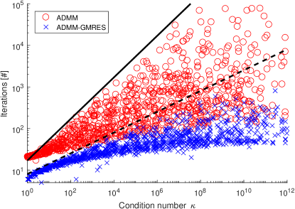
Figure 1: Given the same 1000 randomly-generated problems and using the same parameter choice, ADMM (circles) converges in $O(\sqrt{\kappa})$ iterations while GMRES-accelerated ADMM (crosses) converges in $O(\kappa^{1/4})$ iterations, where $\kappa$ is the condition number.

Under the strong convexity assumptions described in [23], ADMM converges at a linear rate, with a convergence rate dependent on the parameter choice $\beta$ and the problem condition number $\kappa$. A number of previous authors have derived the optimal fixed parameter choice $\beta^{\star}$ that allows ADMM to converge to an $\epsilon$-accurate solution in $O(\sqrt{\kappa}\log\epsilon^{-1})$ iterations [35, 36, 58].

Numerically accelerating this sequence using GMRES, we were surprised to find that an $\epsilon$-accurate solution is consistently computed in $O(\kappa^{1/4}\log\epsilon^{-1})$ iterations, for a square-root factor reduction in the number of iterations. Fig. 1 makes this comparison for 1000 instances of (ECQP) randomly generated using Algorithm 5.2 in Section 5.2 below. The same acceleration was also reliably observed for a wide collection of interior-point Newton subproblems in Section 8.

The order-of-magnitude acceleration is surprising because the $O(\sqrt{\kappa}\log\epsilon^{-1})$ iteration bound is sharp, when considered over all $\kappa$-conditioned (ECQP). Indeed, we give an explicit example of a “hard” instance of (ECQP) in Section 4, and prove that ADMM-GMRES cannot converge for this example at a rate faster than $(\sqrt{\kappa}-1)/(\sqrt{\kappa}+1)$ per iteration. This lower complexity bound is reminiscent of the famous result by Nemirovski and Yudin [53], which states first-order methods cannot minimize every smooth, strongly convex function with condition number $\kappa$ at a rate faster than $(\sqrt{\kappa}-1)/(\sqrt{\kappa}+1)$ per iteration. Indeed, the momentum-accelerated (i.e. “fast”) variants of the gradient method [55] and the projected / proximal descent method [55, 56, 4, 5] are said to be “optimal” precisely because they are able to converge at this rate.

Nevertheless, these numerical results immediately confirm the possibility for an order-of-magnitude acceleration for ADMM under practical settings, using over-relaxation, momentum, or some other scheme. Indeed, one approach is to explicitly extract a $k$-parameter over-relaxation scheme from $k$ iterations of GMRES; see [51] and the references therein. Where convergence is sufficiently rapid, we may consider using GMRES-accelerated ADMM directly as a solution algorithm for (ECQP). In this case, the $O(k^{2})$ time and $O(k)$ memory requirements of GMRES should be balanced against the cost of $k$ iterations of ADMM; see our discussion in Section 2.4.

1.3 Main results

Our primary goal in this paper is to understand why GMRES so frequently achieves an order-of-magnitude acceleration for ADMM. Convergence analysis for Krylov subspace methods is typically formulated as a classic problem in approximation theory—how well can one approximate the eigenvalues of the matrix $I-G(\beta)$ as the roots of an order-$k$ polynomial? In Section 5, we show that the $\kappa^{1/4}$ factor arises because the real eigenvalues of the matrix $I-G(\beta^{\star})$ lie along (a rescaled version of) the interval $[1,\kappa^{1/2}]$, and the Chebyshev polynomial approximates this entire interval with convergence factor $(\kappa^{1/4}-1)/(\kappa^{1/4}+1)$. This is precisely the same mechanism that grants conjugate gradients a square-root factor acceleration over basic gradient descent; see [41, Ch.3] and [67, Ch.6.11].

Within the context of ADMM-GMRES, however, the square-root factor acceleration hinges on two additional assumptions. First, the nonsymmetric iteration matrix $G(\beta)$ should be close to normal, in order for its behavior to be accurately captured by its eigenvalues. Furthermore, $G(\beta)$ also contains complex outliers: eigenvalues with nonzero imaginary parts, which prevent the Chebyshev polynomial from being directly applicable. In Section 5.1, we prove that the $\kappa^{1/4}$ factor will persist if the complex outliers are better conditioned than the real eigenvalues. Our extensive numerical trials found both assumptions to be generic properties of (ECQP), holding for almost all problem instances. As a consequence, convergence in $O(\kappa^{1/4})$ is observed to be generic property for the ADMM-GMRES solution of (ECQP). Although it is difficult to rigorously justify the assumptions, we make a number of heuristic arguments in support of them in Section 5.2 and Section 6.

Much of our analysis is based on the observation that ADMM applied to (ECQP) reduces to a preconditioner for an augmented Lagrangian version of the KKT equations for (ECQP). Within this context, ADMM-GMRES is only one of numerous preconditioned Krylov subspace methods available; see [11] for a comprehensive survey. Indeed, it is closely related to block-triangular [16, 83, 69] and augmented Lagrangian / Uzawa preconditioners [31, 39]. In Section 7, we compare ADMM-GMRES against some classic preconditioners for saddle-point problems, including the block-diagonal preconditioner, variants of the constraint preconditioner, and the Hermitian / Skew-Hermitian splitting preconditioner. Restricting each preconditioner to the same operations used in ADMM, we find that each preconditioner regularly attains its worst-case iteration bound of $O(\sqrt{\kappa})$. By comparison, the ADMM preconditioner converges in $O(\kappa^{1/4})$ iterations for every problem considered. The order-of-magnitude reduction in the number of iterations was able to offset both the higher relative cost of the preconditioner, as well as the need to deploy an expensive Krylov method like GMRES.

It remains an open question whether the order-of-magnitude acceleration would persist for non-quadratic objectives. If the update equations are nonlinear, then ADMM is no longer a matrix iteration, and GMRES acceleration is no longer optimal. Nevertheless, the update equations may be locally well-approximated by their linearization, and a nonlinear version of GMRES like a Newton-Krylov method [17] or Anderson acceleration [78] may prove to be useful.

1.4 Applications to large-scale semidefinite programming

The original motivation of this paper is to solve semidefinite programs (SDPs)

(SDP) $$\underset{Y\succeq 0}{\text{minimize }}\mathrm{tr}\,QY\text{ subject to }\mathrm{tr}\,B_{i}Y=p_{i}\text{ for all }i\in\{1,\ldots,m\},$$

in which the problem data $Q,B_{1},\ldots,B_{m}$ are assumed to be large-and-sparse. Here, each matrix is $\theta\times\theta$ real symmetric, $Y\succeq 0$ indicates that $Y$ is symmetric positive semidefinite. Semidefinite programs are usually solved using an interior-point method; the associated computation cost is dominated by the Newton subproblem

(NEWT) minimize $$\frac{1}{2}\|W^{1/2}(X-\hat{X})W^{1/2}\|_{F}^{2}+p^{T}z$$

subject to $$X+\sum_{i=1}^{m}z_{i}B_{i}=Q,$$

which must be solved at each interior-point iteration, using iteration- and algorithm-specific $\theta\times\theta$ matrices $W$ and $\hat{X}$. In practice, convergence to machine precision almost always occurs within 30-50 iterations, so it is helpful to view the “practical complexity” of (SDP) as a modest constant times the cost of solving (NEWT).

General-purpose interior-point methods solve (NEWT) directly, by performing Gaussian elimination on its linear KKT equations. An important feature of interior-point methods for SDPs is that these KKT equations are typically dense, despite any sparsity in the data matrices $Q,B_{1},\ldots,B_{m}$. As a consequence, the direct approach solves (NEWT) in approximately the same amount of time and memory for highly sparse instances as it does for fully dense ones. In the case of larger problems with $\theta$ and $m$ on the order of thousands, even fitting the KKT equations into memory becomes very difficult.

Alternatively, we can solve (NEWT) using an iterative algorithm, like conjugate gradients (CG) [46, 76, 77, 73] or ADMM [61], as a set of inner iterations within an outer interior-point method. These iterative algorithms have low per-iteration and memory costs that can be further reduced by exploiting sparsity. On the other hand, the resulting interior-point method suffer from “diminishing returns” typical of first-order methods: more and more inner iterations are required for each additional outer iteration. Formally, (NEWT) has condition number $\kappa=\Theta(1/\epsilon^{2})$ at an $\epsilon$-accurate interior-point iterate, so taking the standard $O(\sqrt{\kappa}\log\epsilon^{-1})$ iteration bound for CG and ADMM and the $O(\log\epsilon^{-1})$ iteration bound for the interior-point method, we find that the combined algorithm converges to an $\epsilon$-accurate solution of (SDP) in $O(\epsilon^{-1}(\log\epsilon^{-1})^{2})$ inner iterations. Up to a logarithmic factor, this is the same $O(1/\epsilon)$ iteration bound as obtained by applying a standard first-order method directly to (SDP); see [57, 79]. There seems to be little justification for the added complexities of the interior-point method.

Now, suppose that GMRES-accelerated ADMM is able to solve (NEWT) to $\epsilon$-accuracy in $O(\kappa^{1/4}\log\epsilon^{-1})$ iterations. Then, embedding this accelerated ADMM within an outer interior-point method yields a combined algorithm that converges to an $\epsilon$-accurate solution of (SDP) in $O(\epsilon^{-1/2}(\log\epsilon^{-1})^{2})$ inner iterations. Up to a logarithmic factor, this is the same $O(1/\sqrt{\epsilon})$ iteration bound as “fast” first-order algorithms like Nesterov’s accelerated gradient method [54], FISTA [4], and NESTA [5]. The order-of-magnitude acceleration previously described for the smooth, strongly convex quadratic problem (ECQP) has been extended to the nonsmooth, weakly-convex, non-quadratic problem (SDP) through the use of an outer interior-point loop.

Section 8 tests this idea by embedding ADMM-GMRES within SeDuMi [71], a popular open-source interior-point method written in MATLAB, and using it to solve problems from SDPLIB [14] and the Seventh DIMACS Implementation Challenge [62]. In our results, ADMM-GMRES does indeed solve every instance of (NEWT) in $O(\kappa^{1/4}\log\epsilon^{-1})$ iterations, though the costs associated with GMRES become too high past $\approx 30$ iterations. Restarting ADMM-GMRES every 25 iterations yielded a “fast” first-order method that converged in $O(1/\sqrt{\epsilon})$ iterations for 8 out of the 10 DIMACS problems considered.

1.5 Related work

Accelerating ADMM

When applied to a weakly convex, possibly nonsmooth problem, ADMM has a sublinear error rate, converging to an $\epsilon$-accurate solution within $O(1/\epsilon)$ iterations [42]. Most existing work on accelerating ADMM [38, 60, 44] aim to improve the iteration bound to $O(1/\sqrt{\epsilon})$ by assuming strong convexity and either applying the momentum ideas of Nesterov [54, 56] and Beck and Teboulle [4], or by adopting a “fast” version of the Douglas–Rachford algorithm [28, 19, 63], noting that ADMM is just the Douglas–Rachford algorithm applied to the dual problem [33].

For smooth and strongly convex problems, ADMM converges at a linear rate, producing an $\epsilon$-accurate solution in $O(\sqrt{\kappa}\log\epsilon^{-1})$ iterations [23]. Within this regime, the most widely used acceleration technique is simple over-relaxation, which reliably reduces total iteration count by a small constant [79, 36, 35, 58].

ADMM for SDPs

Semidefinite programs are nonsmooth and weakly convex by construction. While ADMM (or an accelerated variant) can be directly applied to solve (SDP) [79, 59], the resulting iterations converge at a sublinear rate in the worst-case, requiring up to $O(1/\epsilon)$ iterations to produce an $\epsilon$-accurate iterate. In practice, ADMM often performs much better than its worst-case, producing 6-7 accurate digits in just 200-500 iterations over a wide array of test problems [79]. Nevertheless, the algorithm does regularly attain its worst-case bound; several thousand iterations may be required to produce just 2-3 accurate digits [49, 45].

In this paper, we apply ADMM to the inner Newton subproblem (NEWT) within an outer interior-point solution of (SDP). Using GMRES to accelerate ADMM, the number of iterations to $\epsilon$-accuracy is consistently reduced to $O(1/\sqrt{\epsilon})$ iterations, for a square-root factor improvement over directly applying ADMM to (SDP). The $O(1/\epsilon)$ worst-case iteration bound remains unchanged, though our experimental results suggest that the worst-case is difficult to attain.

The per-iteration complexity of ADMM applied to either (SDP) or (NEWT) is at least cubic $\Omega(\theta^{3})$ time and quadratic $\Omega(\theta^{2})$ space, due to the explicit storage of, and algebraic manipulations with, a fully-dense $\theta\times\theta$ matrix variable $Y$. These complexity figures limit the algorithm to medium-sized SDPs, with $\theta$ on the order of a few thousand. However, if the data matrices $Q,B_{1},\ldots,B_{m}$ are sparse with a chordal aggregate sparsity pattern, then it is possible to represent the fully-dense $\theta\times\theta$ matrix variable $Y$ using $\theta$ fully-dense $O(1)\times O(1)$ matrix variables $Y_{1},\ldots,Y_{\theta}$ via a positive semidefinite matrix completion argument; see [32, 52] and also [75] for an extensive survey. This technique, named clique tree conversion or chordal conversion, reduces the per-iteration complexity of ADMM to linear $O(\theta)$ time and space, thereby making it suitable for large-scale SDPs with $\theta$ on the order of tens of thousands [49, 82]. Unfortunately, many large-scale SDPs do not satisfy the chordal sparsity property; for example, it is not satisfied by the large-scale test problems in Section 8.

Iterative solution of the Newton subproblem

The idea of applying a preconditioned iterative solver to the interior-point Newton subproblem dates back to the original Karmarkar interior-point method [46], and remains the standard approach large-scale $\ell_{1}$-regularized regression [18] and network flow problems [50, Chapter 4]. Preconditioners based on sparse matrix ideas, such as incomplete Cholesky factorizations [48] and constraint preconditioning [13], work very well for linear and quadratic programs, but have been less successful for SDP, primarily due to the density of their associated Newton subproblem; see the discussions in [73, 72] for further details.

Preconditioners based on the spectral properties of the Newton subproblem (NEWT), such as the projection preconditioner [73, 72], and the partial Cholesky preconditioner [40, 6], work very well for SDPs. Their key insight is to note that the number of active inequality constraints in (SDP) determines the number of ill-conditioned dimensions in its Newton subproblem (NEWT). If only a few constraints are active, or equivalently, if the solution $Y^{\star}$ to (SDP) is low-rank, then the number of “bad” dimensions in (NEWT) is small, and can be corrected using a low-rank perturbation. The resulting preconditioned problem has a bounded condition number $\kappa=O(1)$ at every $\epsilon$-accurate interior-point iterate.

This paper suggests ADMM as a preconditioner for the Newton subproblem (NEWT). The resulting preconditioned problem has condition number $\kappa=O(1/\sqrt{\epsilon})$ at an $\epsilon$-accurate interior-point iterate under mild technical assumptions. This is a weaker guarantee than the $O(1)$ figure for the spectral preconditioners described above. However, it remains applicable even when the solution $Y^{\star}$ to (SDP) is not low-rank, and the number of “bad” dimensions in (NEWT) is not small. In comparison, the spectral preconditioners are no longer efficient under this regime, and may have costs comparable to that of directly solving the full problem.

Given an arbitrary fully-dense $\theta\times\theta$ algorithm matrix $W$, the per-iteration complexity of an iterative solver applied to (NEWT) is at least cubic $\Omega(\theta^{3})$ time and quadratic $\Omega(\theta^{2})$ space in general. However, if a dual-scaling interior-point method is used (over a primal-dual interior-point method), then $W$ inherits an additional structure: its inverse matrix $W^{-1}$ is sparse, with the same aggregate sparsity pattern as the problem data $Q,B_{1},\ldots,B_{m}$ [8, 75, 7]. Moreover, if the data matrices $Q,B_{1},\ldots,B_{m}$ are sparse with a chordal aggregate sparsity pattern, then $W^{-1}$ can be efficiently factored in linear $O(\theta)$ time and space [20, 2, 81]. Implicitly representing $W$ via its sparse inverse $W^{-1}$ (possibly in factored form) reduces the per-iteration cost of iterative solvers to linear $O(\theta)$ time and space, thereby making them available to large-scale problems with $\theta$ on the order of tens to hundreds of thousands [7, 81].

1.6 Notation

Throughout this paper, we will frequently refer to the condition number $\kappa$, the gradient Lipschitz constant $L$, the strong convexity parameter $\mu$, which are defined in terms of a rescaled objective matrix $\tilde{D}$ in (2.6). The positive integer $k$ is reserved for the iteration index. Accuracy is always measured with respect to the metric $\|\cdot\|_{M}$ defined in (2.10).

The positive integers $n,$ $m,$ $\ell$ refer to the dimensions of the primal-dual variables $x\in\mathbb{R}^{n},$ $z\in\mathbb{R}^{m},$ and $y\in\mathbb{R}^{\ell}$ respectively. Their sum $N=n+m+\ell$ denotes the dimension of the concatenated variable $u=[x;z;y]\in\mathbb{R}^{N}$. In discussing interior-point methods for semidefinite programs in Section 8, the positive integer $\theta$ denotes the order of the semidefinite cone.

Our notation is otherwise standard, with the following exceptions. We use $\Lambda\{A\}$ to refer to the eigenvalues of $A$. The set $\mathbb{P}_{k}$ denotes the space of order-$k$ polynomials. Given a polynomial $p(z)$, we denote its maximum modulus over a compact subset of the complex plane $\mathcal{S}\subset\mathbb{C}$ as $\|p(z)\|_{\mathcal{S}}=\max_{z\in\mathcal{S}}|p(z)|$.

2 ADMM for quadratic problems

Beginning with a choice of the quadratic-penalty / step-size parameter $\beta>0$ and initial points $u^{0}=[x^{0};z^{0};y^{0}]$, ADMM applied to (ECQP) generates iterates

(2.1a) $$x^{k+1} =\arg\min_{x}\frac{1}{2}x^{T}Dx+c^{T}x+\frac{\beta}{2}\|Ax+Bz^{k}-c+y^{k}\|^{2},$$

(2.1b) $$z^{k+1} =\arg\min_{z}p^{T}z+\frac{\beta}{2}\|Ax^{k+1}+Bz-c+y^{k}\|^{2},$$

(2.1c) $$y^{k+1} =y^{k}+(Ax^{k+1}+Bz^{k+1}-c).$$

Some basic algebraic manipulations reveal these to be a matrix-splitting iteration for the (rescaled) augmented Lagrangian KKT system (see e.g. [31, 39])

(2.2) $$\underbrace{\begin{bmatrix}\beta^{-1}D+A^{T}A&A^{T}B&A^{T}\\ B^{T}A&B^{T}B&B^{T}\\ A&B&0\end{bmatrix}}_{H(\beta)}\underbrace{\begin{bmatrix}x\\ z\\ y\end{bmatrix}}_{u}=\underbrace{\begin{bmatrix}A^{T}d-\beta^{-1}c\\ B^{T}d-\beta^{-1}p\\ d\end{bmatrix}}_{v(\beta)},$$

using a Gauss-Seidel–like splitting

(2.3) $$H(\beta)=\underbrace{\begin{bmatrix}\beta^{-1}D+A^{T}A&0&0\\ B^{T}A&B^{T}B&0\\ A&B&-I\end{bmatrix}}_{M(\beta)}-\underbrace{\begin{bmatrix}0&-A^{T}B&-A^{T}\\ 0&0&-B^{T}\\ 0&0&-I\end{bmatrix}}_{N(\beta)}.$$

Indeed, fixing the parameter $\beta$, (2.1) is precisely the linear fixed-point iterations

(2.4) $$u^{k+1}=\underbrace{M(\beta)^{-1}N(\beta)}_{G(\beta)}u^{k}+\underbrace{M(\beta)^{-1}v(\beta)}_{b(\beta)}.$$

ADMM assumes that black-box oracles are available for evaluating matrix-vector products with $(\beta^{-1}D+A^{T}A)^{-1}$, $(B^{T}B)^{-1}$, $A$, $B$, $A^{T}$, and $B^{T}$, without necessarily requiring explicit access to these matrices. The method can be effective only if the oracles are not too expensive to set-up and call. In practice, efficient matrix-implicit implementations frequently arise through problem-specific structure. For example, when the matrices $A$, $B$, and $D$ are large-and-sparse, the matrices $\beta^{-1}D+A^{T}A$ and $B^{T}B$ often admit sparse Cholesky factorizations. After precomputing the factorizations in linear-time, each matrix-vector product with $(\beta^{-1}D+A^{T}A)^{-1}$ or $(B^{T}B)^{-1}$ may be evaluated in linear-time, as the solution of two sparse, triangular linear systems. Alternative structures can also be exploited, including the Kronecker factorization $D=W\otimes W$ for the SDP Newton subproblem in Section 8.1, as well as Toeplitz / Hankel / Circulant matrix structures. For further discussion on these implementation issues, we direct the interested reader to [15, Sec.4.2].

2.1 Sequence acceleration

Let us view ADMM as a black box $T_{\beta}(\cdot)$ that maps a given test point $u$ to its image $T_{\beta}(u)$, in order to rewrite the basic ADMM method as the iterated map

(2.5) $$u^{k+1}=T_{\beta}(u^{k}).$$

Under strong convexity assumptions, (2.5) converges linearly to a unique fixed-point [23]. The matrix $D$ is symmetric positive definite, the matrix $A$ has full row-rank (i.e. $AA^{T}$ is invertible), and the matrix $B$ has full column-rank (i.e. $B^{T}B$ is invertible).

Remark 1.

Given that $A\in\mathbb{R}^{\ell\times n}$ and $B\in\mathbb{R}^{\ell\times m}$, Assumption 2.5 can only be satisfied if $n\geq\ell\geq m$. (Recall that $x\in\mathbb{R}^{n}$, $y\in\mathbb{R}^{\ell}$, $z\in\mathbb{R}^{m}$.)

The convergence rate of (2.5) depends on parameter choice $\beta$ and the problem condition number $\kappa$, defined as the ratio of a gradient Lipschitz parameter $L$ and a strong convexity parameter $\mu$,

(2.6) $$\tilde{D}\triangleq(AD^{-1}A^{T})^{-1},\quad\mu\triangleq\lambda_{\min}(\tilde{D}),\quad L\triangleq\lambda_{\max}(\tilde{D}),\quad\kappa\triangleq L/\mu.$$

In particular, the parameter choice $\beta=\sqrt{\mu L}$ allows an $\epsilon$-accurate solution to be computed in no more than $O(\sqrt{\kappa}\log\epsilon^{-1})$ iterations [35, 36, 58].

Sequence acceleration seeks to find an $\epsilon$-accurate approximation of the fixed point $u^{\star}=T_{\beta}(u^{\star})$ while making as few calls to the black-box oracle as possible. Two popular approaches are over-relaxation, which linearly extrapolates the current step,

(2.7) $$u^{k+1}=u^{k}+\omega_{k}[T_{\beta}(u^{k})-u^{k}],$$

and momentum, which linearly extrapolates the previous step,

(2.8) $$\tilde{u}=u^{k}+\theta_{k}(u^{k}-u^{k-1}),\qquad u^{k+1}=T_{\beta}(\tilde{u}).$$

In each case, the $(k+1)$-th iterate is selected from the plane that crosses the initial point and the $k$ images

(2.9) $$u^{k+1}\in\mathrm{Aff}\{u^{0},T_{\beta}(u^{0}),T_{\beta}(u^{1}),\ldots,T_{\beta}(u^{k})\}.$$

The affine hull linearly extrapolates the information collected from $k$ evaluations of the black-box oracle; the parameters $\theta_{1},\ldots,\theta_{k}$ and $\omega_{1},\ldots,\omega_{k}$ may be viewed as its coordinates. By carefully tuning these parameters, it is possible to select better candidates than the default choice produced by the iterated map (2.5), thereby yielding a sequence $u^{0},u^{1},\ldots,u^{k}$ with an accelerated convergence rate.

2.2 The optimality of GMRES

Let the black-box oracle $T_{\beta}(\cdot)$ be affine, meaning that there exists some matrix $G(\beta)$ and vector $b(\beta)$ such that $T_{\beta}(u)=G(\beta)u+b(\beta)$. Furthermore, let us measure the accuracy of a test point $u$ using an implicit but easily computable Euclidean metric

(2.10) $$\|u-u^{\star}\|_{M}\triangleq\|u-[G(\beta)u+b(\beta)]\|=\|[I-G(\beta)](u-u^{\star})\|.$$

Then, the affine search space (2.9) reduces to a Krylov subspace

(2.11) $$u^{k+1}\in u^{0}+\mathrm{span}\{r,Gr,\ldots,G^{k}r\}$$

where $G\equiv G(\beta)$ and $r=u^{0}-[G(\beta)u^{0}+b(\beta)]$, and the problem of selecting the best candidate from the Krylov subspace (2.11) is numerically solved by GMRES. We defer to standard texts for its implementation details, e.g. [67, Alg. 6.9] or [67, Alg. 6.10], and only note that the algorithm can be viewed as a “black-box” that solves the following projected least-squares problem at the $k$-th iteration:

(2.12) $$\mathbf{GMRES}_{k}(A,b) =\arg\min\left\{\|b-Ax\|_{2}:x\in\mathrm{span}\{b,Ab,\ldots,A^{k-1}b\}\right\},$$

in $\Theta(k^{2}N)$ flops, $\Theta(kN)$ memory, and $k$ matrix-vector products with $A$. Consider the following algorithm. [ADMM-GMRES] Input: The update operator $T_{\beta}$ that implements (2.1) as $u^{k+1}=T_{\beta}(u^{k})$; Initial point $u^{0}$; Number of iterations $k$.

1. Precompute and store $T_{\beta}(u^{0})=G(\beta)u^{0}+b(\beta)$ and $r=u^{0}-T_{\beta}(u^{0})$;

2. Call $\Delta u=\mathbf{GMRES}_{k}(I-G(\beta),\,r)$, while evaluating each matrix-vector product as $[I-G(\beta)]h=h-[T_{\beta}(u_{0}+h)-T_{\beta}(u^{0})]$;

3. Output $u^{k}=u^{0}-\Delta u$.

The optimality of GMRES in (2.12) guarantees $\|u^{k}-u^{\star}\|_{M}$ to be smaller than that of regular ADMM, as well as any accelerated variant that selects its $k$-th iterate $u^{k}$ from (2.9). In other words, no linearly extrapolating sequence acceleration scheme, based on momentum, over-relaxation, or otherwise, can converge faster than GMRES when viewed under this metric.

2.3 ADMM as a preconditioner

The fixed-point equation associated with the ADMM iterations (2.4)

(2.13) $$u^{\star}-G(\beta)u^{\star}=b(\beta),$$

is a linear system of equations when $\beta$ is held fixed, which can be solved using GMRES. In the previous subsection, we named the resulting method ADMM-GMRES, and viewed it as an optimally accelerated version of ADMM. Equivalently, (2.13) is also the left-preconditioned system of equations

(2.14) $$M^{-1}(\beta)[H(\beta)u^{\star}-v(\beta)]=0\qquad\Leftrightarrow\qquad\text{(\ref{eq:admm_fixed})},$$

where $H$ and $v$ comprise the augmented Lagrangian KKT system in (2.2), and $M$ is the preconditioner matrix defined in (2.3). Note that the ADMM iteration matrix satisfies $G(\beta)=I-M^{-1}(\beta)H(\beta)$ by definition. In turn, ADMM-GMRES is equivalent to a preconditioned GMRES solution of the augmented KKT system $H(\beta)u=v(\beta)$ using $M(\beta)$ as the preconditioner.

2.4 Reducing the cost of GMRES

A significant shortcoming of GMRES is its need to store and manipulate an $N\times k$ dense matrix at the $k$-th iteration. Its $\Theta(k^{2}N)$ time and $\Theta(kN)$ memory requirements become unsustainable once $k$ grows large. It was proved by Faber and Manteuffel that these complexity figures cannot be substantially reduced without destroying the optimal property of GMRES [29]. Hence, if many GMRES iterations are desired, then we must give up on its optimality and adopt a limited-memory heuristic.

One limited-memory approach is to periodically restart GMRES: after $p$ iterations, the final iterate is extracted, and used as the initial point for a new set of $p$ iterations. An issue with the resulting algorithm, known as GMRES($p$), is that it can stall, meaning that it may fail to make further progress after a certain number of iterations. Alternatively, a Krylov method based on Lanczos biorthogonalization may be used, including BiCG, QMR and their transpose-free variants; see [67]. These are entirely heuristic, but tend to work well when GMRES converges quickly, and do not stall as easily as restarted GMRES. QMR is often preferred over BiCG for being more stable and for having a convergence analysis somewhat related to GMRES.

Limited-memory variants of ADMM-GMRES can be developed by viewing it as a preconditioned GMRES solution of the augmented KKT system $H(\beta)u=v(\beta)$ in (2.2) using the matrix $M(\beta)$ in (2.3) as the preconditioner. For example, we obtain ADMM-GMRES($p$) and ADMM-QMR by using GMRES($p$) and QMR in place of regular GMRES, respectively. Fig. 2 compares ADMM with ADMM-GMRES and these two limited-memory variants, as applied to two problems of comparable conditioning. In the first, “easy” example, all limited-memory variants of ADMM-GMRES outperform basic ADMM, with ADMM-QMR converging almost as rapidly as ADMM-GMRES, despite requring far less time and memory. But in the second, “difficult” example, all of these limited-memory variants stall, or get close to stalling. Only ADMM-GMRES is able to converge at the desired $(\kappa^{1/4}-1)/(\kappa^{1/4}+1)$ rate.

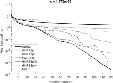
(a)

(b)

Figure 2: Comparison of ADMM with ADMM-GMRES and its limited-memory variants: (a) an “easy” example; (b) a “difficult” example.

3 GMRES convergence analysis

Krylov subspace methods like GMRES are closely associated with the idea of approximating a matrix inverse using a low-order matrix polynomial. To explain, consider substituting the constraints of the GMRES least-squares problem (2.12) into its objective, to yield

(3.1) $$\|b-Ax^{k}\|=\min_{\alpha_{1},\ldots,\alpha_{k}}\left\|b-A\left(\sum_{j=1}^{k}\alpha_{j}A^{j-1}b\right)\right\|=\min_{p\in\mathbb{P}_{k-1}}\|[I-Ap(A)]b\|.$$

If there exists an accurate low-order matrix polynomial approximation $p(A)$ for the matrix inverse $A^{-1}$, then $Ap(A)\approx I$ and $\|[I-Ap(A)]b\|\approx 0$. GMRES must converge rapidly, since it optimizes over all polynomials in (3.1).

Equivalently, we may solve the residual minimization problem

(3.2) $$\min_{p\in\mathbb{P}_{k-1}}\left\{\|q(A)b\|:q(z)=1-zp(z)\right\}=\min_{\begin{subarray}{c}q\in\mathbb{P}_{k}\\ q(0)=1\end{subarray}}\|q(A)b\|,$$

and recover $p(A)$ via $p(z)=z^{-1}(q(z)-1)$. Equation (3.2) is the standard tool for analyzing the convergence of optimal Krylov subspace methods like GMRES; see [41, 25, 67]. For each $k\in\{1,2,\ldots\}$, the typical proof constructs a heuristic polynomial $h_{k}(z)\in\mathbb{P}_{k}$ satisfying $h_{k}(0)=1$, and demonstrates that the induced 2-norm of the matrix polynomial $h_{k}(A)$ converges geometrically, as in $\|h_{k}(A)\|\leq\alpha\varrho^{k}$. Then, since GMRES optimizes over all polynomials in (3.2), it must converge at least as quickly as this particular choice of polynomial:

(3.3) $$\min_{\begin{subarray}{c}q\in\mathbb{P}_{k}\\ q(0)=1\end{subarray}}\|q(A)b\|\leq\|h_{k}(A)b\|\leq\|b\|\alpha\varrho^{k}.$$

Hence, we conclude that GMRES converges at the asymptotic rate of $\varrho$, requiring no more than $(1-\varrho)^{-1}\log(\alpha\epsilon^{-1})$ iterations to converge to an $\epsilon$-accurate iterate.

In this section, we will simplify the residual minimization problem (3.2) associated with the matrix $A\leftarrow[I-G(\beta)]$ to an easier one associated with the $\ell\times\ell$ nonsymmetric matrix

(3.4) $$K(\beta)\triangleq\begin{bmatrix}Q^{T}\\ -P^{T}\end{bmatrix}\left[(\beta^{-1}\tilde{D}+I)^{-1}-(\beta\tilde{D}^{-1}+I)^{-1}\right]\begin{bmatrix}Q&P\end{bmatrix},$$

in which $\tilde{D}=(AD^{-1}A^{T})^{-1}$ and $B=\left[\begin{smallmatrix}Q&P\end{smallmatrix}\right]\left[\begin{smallmatrix}R\\ 0\end{smallmatrix}\right]$ is the QR decomposition of $B$. (Recall that $\ell$ is the number of rows in $A$, $B$, as well as the dimension of the Lagrange multiplier $y$.) We begin by showing that only $\ell\leq\frac{1}{2}N$ eigenvalues of the $N\times N$ iteration matrix $G(\beta)$ are nonzero, and these have values that coincide with the eigenvalues of $G_{22}(\beta)=\frac{1}{2}I+\frac{1}{2}K(\beta)$.

Lemma 3.1.

Let $B=\left[\begin{smallmatrix}Q&P\end{smallmatrix}\right]\left[\begin{smallmatrix}R\\ 0\end{smallmatrix}\right]$ be the QR decomposition of $B$. Then the ADMM iteration matrix $G(\beta)$ defined in (2.4) has a block decomposition

(3.5) $$G(\beta)=\left[\begin{array}[]{c|cc|c}I_{n}&0&0&0\\ 0&R^{-1}&0&0\\ 0&0&P&Q\end{array}\right]\left[\begin{array}[]{c|c|c}0_{n}&G_{12}(\beta)&G_{13}(\beta)\\ \hline\cr 0&G_{22}(\beta)&G_{23}(\beta)\\ \hline\cr 0&0&0_{m}\end{array}\right]\left[\begin{array}[]{ccc}I_{n}&0&0\\ \hline\cr 0&R&0\\ 0&0&P^{T}\\ \hline\cr 0&0&Q^{T}\end{array}\right],$$

into blocks of size $n$, $\ell$, and $m$ respectively, in which the constituent matrices are

$$G_{12}(\beta)=-\beta D^{-1}A^{T}(\beta^{-1}\tilde{D}+I)^{-1}\begin{bmatrix}Q&P\end{bmatrix},$$

$$G_{13}(\beta)=-\beta D^{-1}A^{T}(\beta^{-1}\tilde{D}+I)^{-1}Q,$$

$$G_{22}(\beta)=\frac{1}{2}I+\frac{1}{2}K(\beta),\qquad G_{23}(\beta)=\begin{bmatrix}Q^{T}\\ -P^{T}\end{bmatrix}(\beta\tilde{D}^{-1}+I)^{-1}Q,$$

$K(\beta)$ is defined in (3.4), and $\tilde{D}=(AD^{-1}A^{T})^{-1}$.

Proof 3.2.

Follows from direct computation and applications of the Sherman–Morrison–Woodbury identity.

Remark 2.

The special structure of $K(\beta)$ allows its singular values to be explicitly stated. In particular,

(3.6) $$\|K(\beta)\|=\frac{\gamma-1}{\gamma+1}\quad\text{where }\gamma=\max\left\{\frac{L}{\beta},\frac{\beta}{\mu}\right\},$$

so the eigenvalues of $K(\beta)$ are contained within the disk on the complex plane centered at at the origin, with radius $(\gamma-1)/(\gamma+1)$. This is an important characterization of $K(\beta)$ that we will use extensively in Sections 4 & 5.

Furthermore, the block pattern in the Schur decomposition (3.5) suggests that the Jordan block associated with each zero eigenvalue of $G(\beta)$ is at most size $2\times 2$. After two iterations, ADMM becomes entirely dependent upon the inner iteration matrix $G_{22}(\beta)$.

Corollary 3.

Given $\beta>0$ and any polynomial $p(\cdot)$, we have

$$\|p(G(\beta))\,G^{2}(\beta)\|\leq c_{0}\left(1+\beta\|D^{-1}A^{T}\|\right)\|p(G_{22}(\beta))\|,$$

where $c_{0}=2\max\{\sigma_{\max}(B),1/\sigma_{\min}(B),\sigma_{\max}(B)/\sigma_{\min}(B)\}$.

Proof 3.3.

Let us write $G\equiv G(\beta)$. For each matrix monomial, we substitute Lemma 3.1 and note that the following holds for all $j\geq 0$

$$G^{j}=U\left[\begin{array}[]{c|c|c}0&G_{12}&G_{13}\\ \hline\cr 0&G_{22}&G_{23}\\ \hline\cr 0&0&0\end{array}\right]^{j+2}U^{-1} =U\left[\begin{array}[]{c}G_{12}\\ \hline\cr G_{22}\\ \hline\cr 0\end{array}\right]G_{22}^{j}\left[\begin{array}[]{c|c|c}0&G_{22}&G_{23}\end{array}\right]U^{-1}.$$

Repeating this argument for each monomial in $p(\cdot)$, we find that

$$\|p(G)\,G^{2}\| \leq\kappa_{U}\|\begin{bmatrix}G_{12}&G_{22}\end{bmatrix}\|\|\begin{bmatrix}G_{22}&G_{23}\end{bmatrix}\|\|p(G_{22})\|,$$

$$\leq\kappa_{U}(\beta\|D^{-1}A^{T}\|+1)(1+1)\|p(G_{22})\|,$$

where $\kappa_{U}=\|U\|\|U^{-1}\|=\max\{\sigma_{\max}(B),1/\sigma_{\min}(B),\sigma_{\max}(B)/\sigma_{\min}(B)\}$.

Accordingly, the residual minimization problem (3.2) posed over $G(\beta)$ is reduced to a simpler problem over $K(\beta)$ after two iterations.

Lemma 3.4.

Fix $\beta>0$ and initial point $u^{0}$. Let $u^{k}$ be the iterate generated at the $k$-th iteration of ADMM-GMRES (Algorithm 2.2). Then the following holds for all $k\geq 2$

(3.7) $$\frac{\|u^{k}-u^{\star}\|_{M}}{\|u^{0}-u^{\star}\|_{M}}\leq(c_{0}+c_{1}\beta)\min_{\begin{subarray}{c}p\in\mathbb{P}_{k-2}\\ p(1)=1\end{subarray}}\|p(K(\beta))\|,$$

where $K(\beta)$ is defined in (3.4), $\|\cdot\|_{M}$ is defined in (2.10), $\mathbb{P}_{k}$ is the space of order-$k$ polynomials, and $c_{0},c_{1}$ are constants.

Proof 3.5.

Substituting $A\leftarrow(I-G(\beta))$ and $b\leftarrow r$ into (3.2) yields

$$\min_{\begin{subarray}{c}p\in\mathbb{P}_{k}\\ p(0)=1\end{subarray}}\|p(I-G(\beta))r\|\overset{\text{(a)}}{=}\min_{\begin{subarray}{c}p\in\mathbb{P}_{k}\\ p(1)=1\end{subarray}}\|p(G(\beta))r\|\\ \overset{\text{(b)}}{\leq}\|r\|c(\beta)\min_{\begin{subarray}{c}p\in\mathbb{P}_{k-2}\\ p(1)=1\end{subarray}}\|p(G_{22}(\beta))\|\overset{\text{(c)}}{=}\|r\|c(\beta)\min_{\begin{subarray}{c}p\in\mathbb{P}_{k-2}\\ p(1)=1\end{subarray}}\|p(K(\beta))\|.$$

Equality (a) shifts the polynomials $p(1-z)\leftrightarrow p(z^{\prime})$, which also shifts the constraint point from $z=0$ to $z^{\prime}=1$. Inequality (b) takes the heuristic choice of $p(z)=z^{2}q(z)$ with an order $k-2$ polynomial $q$, and substitutes Corollary 3. Equality (c) then shifts and scales the polynomials $p(z)\leftrightarrow p(\frac{1}{2}+\frac{1}{2}z^{\prime})$, keeping the constraint point $z=1$ at $z^{\prime}=1$.

4 Worst-case behavior

When applied to (ECQP), ADMM converges at the rate of $1-1/\sqrt{\kappa}$ with the parameter choice of $\beta=\sqrt{\mu L}$; a number of previous authors have established versions of the following statement [23, 36, 35, 58].

Proposition 4.1.

The $k$-th iterate of ADMM with $k\geq 2$ satisfies

$$\frac{\|u^{k}-u^{\star}\|_{M}}{\|u^{0}-u^{\star}\|_{M}}\leq(c_{0}+c_{1}\beta)\left(\frac{\gamma}{\gamma+1}\right)^{k-2}$$

where $\gamma=\max\{L/\beta,\beta/\mu\}$, and $c_{0},c_{1}$ are constants. The bound is sharp up to a multiplicative constant.

Proof 4.2.

The residuals satisfy $r^{k}=G^{k}(\beta)r^{0}$, so $\|r^{k}\|/\|r^{0}\|\leq\|G^{k}(\beta)\|$. To establish the inequality, we substitute the bound $\|G_{22}^{k}\|\leq(\frac{1}{2}+\frac{1}{2}\|K\|)^{k}$ from Lemma 3.1 and the value of $\|K\|$ from Remark 2 into Corollary 3. To prove sharpness, we take $n=\ell=2m$ and set $A=I_{n}$, $B=[I_{m},0_{m}]^{T}$, and $D$ diagonal. Then, both $G_{22}$ and $K$ are diagonal by construction, so $\|G_{22}^{k}\|=(\frac{1}{2}+\frac{1}{2}\|K\|)^{k}$ trivially holds.

Let us use Lemma 3.4 to prove a similar statement for ADMM-GMRES.

Theorem 4.3.

The $k$-th iteration of ADMM-GMRES satisfies

$$\frac{\|u^{k}-u^{\star}\|_{M}}{\|u^{0}-u^{\star}\|_{M}}\leq\left(c_{0}+c_{1}\beta\right)\left(\frac{\gamma-1}{\gamma+1}\right)^{k-2}$$

where $\gamma=\max\{L/\beta,\beta/\mu\}$, and $c_{0},c_{1}$ are constants. The bound is sharp up to a multiplicative constant.

Proof 4.4.

To establish the inequality, we set $p(z)$ in Lemma 3.4 to be the monomial $p(z)=z^{k-2}$ and take $\|K^{k}\|\leq\|K\|^{k}$. To prove sharpness, we take $n=\ell=2m$ and give a problem construction satisfying $\|K^{k}\|=\|K\|^{k}$ whose optimal polynomial is precisely $p^{\star}(z)=z^{k-2}$. Consider

$$A=I_{n},\qquad D=\begin{bmatrix}\frac{1}{\sqrt{\kappa}}I_{m}&0\\ 0&\sqrt{\kappa}I_{m}\end{bmatrix},$$

$$B=\begin{bmatrix}\cos\Theta\\ \sin\Theta\end{bmatrix}\text{ where }\Theta=\frac{\pi}{2n}\mathrm{diag}\,(1,3,5,\ldots,n-1).$$

By inspection, $\mu=1/\sqrt{\kappa}$, $L=\sqrt{\kappa}$, and $L/\mu=\kappa$, and $K(\sqrt{\mu L})$ is a scaled orthogonal matrix

$$K(\sqrt{\mu L})=\frac{\sqrt{\kappa}-1}{\sqrt{\kappa}+1}\begin{bmatrix}\cos 2\Theta&-\sin 2\Theta\\ \sin 2\Theta&\cos 2\Theta\end{bmatrix}$$

whose $n$ eigenvalues lie evenly spaced along the circumference of a circle centered at the origin with radius $a=\|K(\sqrt{\mu L})\|=\frac{\sqrt{\kappa}-1}{\sqrt{\kappa}+1}$. The associate eigenvalue approximation problem is bound:

$$\min_{\begin{subarray}{c}p\in\mathbb{P}_{k-2}\\ p(1)=1\end{subarray}}\|p(K(\sqrt{\mu L}))\|\overset{\text{(a)}}{=}\min_{\begin{subarray}{c}p\in\mathbb{P}_{k-2}\\ p(1)=1\end{subarray}}\max_{i\in\{1,\ldots,n\}}|p(a\omega^{i})|\overset{\text{(b)}}{\leq}\min_{\begin{subarray}{c}p\in\mathbb{P}_{k-2}\\ p(1)=1\end{subarray}}\max_{\begin{subarray}{c}\lambda\in\mathbb{C}\\ |\lambda|=a\end{subarray}}|p(\lambda)|\overset{\text{(c)}}{=}a^{k-2},$$

where $\omega=\exp(\sqrt{-1}\frac{2\pi}{n})$ is the $n$-th root of unity. Step (a) makes a unitary eigendecomposition for the normal matrix $K(\sqrt{\mu L})=XSX^{*}$, where $XX^{*}=X^{*}X=I$, and notes that $\|p(K(\sqrt{\mu L}))\|=\|Xp(S)X^{*}\|=\|p(S)\|$. Step (b) encompasses the roots of unity $\omega^{i}$ within the unit circle $\{z\in\mathbb{C}:|z|=1\}$. Step (c) applies the closed-form solution $p^{\star}(z)=z^{k-2}$ due to Zarantonello (see [64] for a proof, or [25] for a more intuitive explanation). In the limit $n\to\infty,$ the roots of unity converge uniformly to the unit circle, and the inequality (b) converge uniformly towards an equality.

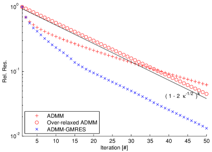
Figure 3: The problem construction in the proof of Theorem 4.3 places the eigenvalues of $K(\beta)$ in a circle, so ADMM-GMRES convergences at the same asymptotic rate as over-relaxed ADMM with $\omega=2$.

Setting $\beta=\sqrt{\mu L}$ minimizes value of $\gamma=\max\{L/\beta,\beta/\mu\}$. This parameter choice allows ADMM to converge to an $\epsilon$-accurate solution in

(4.1) $$\left\lceil(\sqrt{\kappa}+1)\log\left(\frac{c_{0}+c_{1}\beta}{\epsilon}\right)\right\rceil\text{ iterations,}$$

and ADMM-GMRES to do the same in

(4.2) $$\left\lceil\frac{1}{2}(\sqrt{\kappa}+1)\log\left(\frac{c_{0}+c_{1}\beta}{\epsilon}\right)\right\rceil\text{ iterations.}$$

We see that ADMM-GMRES is only a factor of two better than basic ADMM. In the worst case, GMRES will not be able to yield a substantial acceleration over the basic ADMM method. This is easily verified numerically; see Fig. 3.

Indeed, the optimal polynomial used to prove Theorem 4.3 may be extracted and explicitly applied as a successive over-relaxation scheme.

Corollary 4.

Consider the successive over-relaxation (SOR) iterations

$$u^{1} =G(\beta)u^{0}+v(\beta),\qquad u^{2}=G(\beta)u^{1}+v(\beta),$$

$$u^{j+1} =(1-\omega)u^{j}+\omega[G(\beta)u^{j}+v(\beta)]\quad\forall j\in\{3,\ldots,k\}$$

with $\beta=\sqrt{\mu L}$ and $\omega=2$. Then the $k$-th iterate $u^{k}$ satisfies the bound in Theorem 4.3.

Proof 4.5.

The SOR residuals satisfy $r^{k}=q(G)r^{0}$ where $q(z)=\prod_{i=1}^{k}[(1-\omega_{j})+\omega_{j}z]$. Collocating its roots with those of the optimal polynomial $p^{\star}(z)$ in the proof of Theorem 4.3 yields the desired iterates.

This is precisely over-relaxed ADMM using the parameter choice of $\omega=2$, which was shown to be optimal by several previous authors [21, 35, 58].

5 Explaining Convergence in $O(\kappa^{1/4})$ Iterations

In order to understand the circumstances that allow the ADMM-GMRES converge an order-of-magnitude faster than basic ADMM, we make the following assumption. [$\kappa_{X}$ is bounded] For a fixed $\beta>0$, the matrix $K(\beta)$, defined in (3.4), is diagonalizable. Furthermore, it has an eigendecomposition $K(\beta)=XSX^{-1}$ whose matrix-of-eigenvectors $X$ has a bounded condition number $\kappa_{X}=\|X\|\|X^{-1}\|$. Intuitively, we assume that the matrix $K(\beta)$ is close to normal, so that its behavior can be accurately described by its eigenvalues alone; we will return to this point later in Section 6. Substituting $\|p(K)\|=\|Xp(S)X^{-1}\|\leq\|X\|\|p(S)\|\|X^{-1}\|$ reduces the residual minimization problem in Lemma 3.4 to an eigenvalue approximation problem (see e.g. [68])

(5.1) $$\frac{\|u^{k}-u^{\star}\|_{M}}{\|u^{0}-u^{\star}\|_{M}}\leq(c_{0}+c_{1}\beta)\kappa_{X}\min_{\begin{subarray}{c}p\in\mathbb{P}_{k-2}\\ p(1)=1\end{subarray}}\|p(z)\|_{\Lambda},$$

where we have used the maximum modulus notation

$$\|p(z)\|_{\Lambda}\triangleq\max_{z\in\Lambda}|p(z)|,\qquad\Lambda\triangleq\{\lambda_{1},\ldots,\lambda_{m}\}.$$

In this new problem, our objective is to construct a low-order polynomial whose zeros are approximately the eigenvalues of $K(\beta)$.

Problem (5.1) is made easier by enclosing the eigenvalues $\Lambda$ within the disk $\mathcal{D}=\{z\in\mathbb{C}:|z|\leq a\}$ mentioned earlier in Remark 2, with radius

(5.2) $$a\triangleq\frac{\gamma-1}{\gamma+1}\text{ where }\gamma=\max\left\{\frac{L}{\beta},\frac{\beta}{\mu}\right\}.$$

In view of Theorem 4.3, this enclosure $\Lambda\subset\mathcal{D}$ is sharp: there exists a choice of problem data $A,B,D$ to place $\Lambda$ right along the boundary $\partial\mathcal{D}$. The associated optimal polynomial is simply $p^{\star}(z)=z^{k}$, but this causes ADMM-GMRES to converge at the same rate as regular ADMM.

In order to improve upon the $O(\sqrt{\kappa})$ iteration estimate from Theorem 4.3, we must introduce additional information about the distribution of eigenvalues within the interior of the disk. Suppose, in particular, that all of our eigenvalues were also real, i.e. $\Lambda\subset\mathbb{R}$. Then the corresponding approximation problem over the real interval $\mathcal{I}\triangleq\mathbb{R}\cap\mathcal{D}$ has a closed-form solution attributed to Chebyshev (see [41, Ch.3] or [67, Sec.6.11.1])

(5.3) $$\min_{\begin{subarray}{c}p\in\mathbb{P}_{k}\\ p(1)=1\end{subarray}}\|p(z)\|_{\mathcal{I}}=\frac{1}{|T_{k}(1/a)|}\leq 2\left(\frac{\sqrt{\gamma}-1}{\sqrt{\gamma}+1}\right)^{k},$$

attained by $p^{\star}(z)=T_{k}(z/a)/|T_{k}(1/a)|$ where $T_{k}(z)$ is the order-$k$ Chebyshev polynomial of the first kind. Using the Chebyshev polynomial to solve the eigenvalue approximation problem (5.1) yields an optimal convergence rate of $(\kappa^{1/4}-1)/(\kappa^{1/4}+1)$ for the parameter choice $\beta=\sqrt{\mu L}$. In other words, ADMM-GMRES converges to an $\epsilon$-accurate solution in $O(\kappa^{1/4})$ iterations, for an order of magnitude improvement over its worst-case.

5.1 Damping the outlier eigenvalues

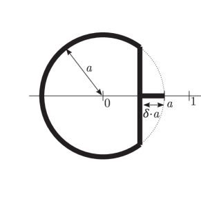
(a)

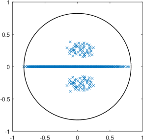
(b)

Figure 4: The enclosure $\mathcal{I}\cup\mathcal{C}$ bounds the outlier eigenvalues away from the right-side of the disk by the distance $\delta\cdot a$: (a) graphical illustration; (b) numerical example, for a problem with $n=500$, $m=400$, $\ell=50$.

In practice, $K(\beta)$ also has a number of eigenvalues with nonzero imaginary parts. These eigenvalues prevent (5.3) from being directly applicable, so we refer to them as outlier eigenvalues. The issue of outliers is standard in Krylov subspace methods. If the number of outliers is small, then a standard technique is to annihilate them one at a time, and to apply a Chebyshev approximation to the remaining eigenvalues that lie along a line; see [41, p.53] or [25, Sec.5]. In our numerical experiments, however, the number of outlier eigenvalues was often observed to be quite large.

Instead, let us assume a different structure: that the outlier eigenvalues are better conditioned than the real eigenvalues. Rather than annihilating them one at a time, it may be sufficient to “dampen” their effect using a few fixed-point iterations, like in multigrid methods. Then, the Chebyshev approximation can be used to approximate the remaining purely-real but poorly-conditioned eigenvalues. Since GMRES is optimal, it must converge faster than this heuristic approach.

Consider the eigenvalue enclosure $\Lambda\{K\}\subset\mathcal{I}\cup\mathcal{C}$, where $\mathcal{I}=\mathbb{R}\cap\mathcal{D}$ is the same real interval considered in the previous section, and

(5.4) $$\mathcal{C} \triangleq\{z\in\mathcal{D}:\mathrm{Re}\{z\}\leq\delta\cdot a\},\qquad\delta\triangleq 1-\max_{\begin{subarray}{c}\lambda\in\Lambda\{K(\beta)\}\\ \mathrm{Im}\,\lambda\neq 0\end{subarray}}\frac{\mathrm{Re}\,\lambda}{\|K(\beta)\|}\geq 0$$

is used to encompasses the outlier eigenvalues; an illustration is shown in Fig. 4. We view the quantity $\delta^{-1}$ as a relative condition number of $\mathcal{C}$, due to the following result.

Lemma 5.1.

The approximation problem for $\mathcal{C}$ in (5.4) is bounded

$$\min_{\begin{subarray}{c}p\in\mathbb{P}_{k}\\ p(1)=1\end{subarray}}\|p(z)\|_{\mathcal{C}}\leq\left(\frac{2a}{1+a}\right)^{k}\left(1-\frac{\delta}{2}\right)^{k/2},$$

using the polynomial $p(z)=(z+a)^{k}/(1+a)^{k}$.

Proof 5.2.

We use the over-relaxation polynomial $p(z)=(z+\omega)^{k}(1+\omega)^{-k}$ to approximate $\mathcal{C}$. Since $\omega>0$, the maximum modulus is attained at $z^{\star}=\arg\max_{z\in\mathcal{C}}|p(z)|=a\left[(1-\delta)\pm j\sqrt{1-(1-\delta)^{2}}\right]$. Now,

$$\frac{|z^{\star}+\omega|^{2}}{(1+\omega)^{2}}=\frac{[a(1-\delta)+\omega]^{2}+a^{2}[1-(1-\delta)^{2}]}{(1+\omega)^{2}}=\frac{(a+\omega)^{2}}{(1+\omega)^{2}}\left(1-\frac{2a\delta\omega}{(a+\omega)^{2}}\right).$$

Setting $\omega=a$ maximizes the ratio $2\delta\omega/(a+\omega)^{2}$ and yields the desired bound.

Fixing $\delta>0$, the error over $\mathcal{C}$ can be dampened to some prescribed accuracy in a fixed number of iterations, independent of all other considerations. This is the central insight that we use in our new iteration estimate; so long as $\delta>0$, ADMM-GMRES will converge in $O(\kappa^{1/4})$ iterations.

Theorem 5.3.

Under Assumption 5, the $k$-th iterate of ADMM-GMRES satisfies

(5.5) $$\frac{\|u^{k}-u^{\star}\|_{M}}{\|u^{0}-u^{\star}\|_{M}}\leq 2(c_{0}+\beta c_{1})\kappa_{X}\left(\frac{\sqrt{\gamma}-1}{\sqrt{\gamma}+1}\right)^{\delta(k-2)/6},$$

where $\delta$ is defined in (5.4), and $c_{0},c_{1},\kappa_{X}$ are constants.

Our proof solves the approximation problem (5.1) over $\mathcal{I}\cup\mathcal{C}\supset\Lambda$ using the following polynomial

$$p_{k}(z)\triangleq\left(\frac{z+a}{1+a}\right)^{\eta}\frac{T_{\xi}(z/a)}{|T_{\xi}(1/a)|},\qquad\xi\triangleq k-\eta,$$

which is constructed as the product of $\eta$ fixed-point iterations and an order-$\xi$ Chebyshev polynomial from (5.3). Intuitively, each increment of $\xi$ decreases global error by $(\sqrt{\gamma}-1)/(\sqrt{\gamma}+1)$, but also increases the relative error between $\mathcal{C}$ and $\mathcal{I}$ by a constant factor. To smooth this error between the two regions, we increment $\eta$ by a fixed number determined by Lemma 5.1. Alternating between decrementing the global error and smoothing the relative error allows us to converge at the overall accelerated rate of $(\sqrt{\gamma}-1)/(\sqrt{\gamma}+1)$.

Proof 5.4.

Noting that $\|p_{k}(z)\|_{\Lambda}\leq\|p_{k}(z)\|_{\mathcal{I}\cup\mathcal{C}}=\max\left\{\|p_{k}(z)\|_{\mathcal{I}},\|p_{k}(z)\|_{\mathcal{C}}\right\}$, we bound each component

(5.6) $$\|p_{k}(z)\|_{\mathcal{C}} \leq\left(\frac{2a}{1+a}\right)^{\eta}\left(1-\frac{\delta}{2}\right)^{\eta/2}\frac{(1+\sqrt{2})^{\xi}}{T_{\xi}(1/a)},$$

(5.7) $$\|p_{k}(z)\|_{\mathcal{I}} =\left(\frac{2a}{1+a}\right)^{\eta}\frac{1}{T_{\xi}(1/a)}\leq 2\left(\frac{\sqrt{\gamma}-1}{\sqrt{\gamma}+1}\right)^{\xi},$$

using Lemma 5.5 and $\max_{|z|\leq 1}|T_{n}(z)|\leq(1+\sqrt{2})^{n}$. We will pick the ratio $\eta/\xi$ to satisfy

(5.8) $$\left(1-\frac{\delta}{2}\right)^{\eta/\xi}\leq\frac{1}{(1+\sqrt{2})^{2}},$$

so that we have $\|p_{k}(z)\|_{\mathcal{I}}\geq\|p_{k}(z)\|_{\mathcal{C}}$. Viewing $\eta/\xi$ as an “iteration estimate” to guarantee a constant error reduction of $\epsilon=1/(1+\sqrt{2})^{2}$ over $\mathcal{C}$, we take logarithms and obtain $\eta/\xi\geq 2\delta^{-1}\log\epsilon^{-1}=c_{3}\delta^{-1}$ and $\xi\geq\delta(k-2)/6$, noting that $\delta\leq 2$. With $\|p_{k}(z)\|_{\mathcal{I}}=\|p_{k}(z)\|_{\mathcal{I}\cup\mathcal{C}}$ now guaranteed, we take the second expression in (5.7) to be the global error estimate $\|p_{k}(z)\|_{\mathcal{I}}\geq\|p_{k}(z)\|_{\Lambda}$ for (5.1).

Theorem 5.3 says that ADMM-GMRES will converge to an $\epsilon$-accurate solution in

$$2+\left\lceil\frac{6(\kappa^{1/4}+1)}{\delta}\log\left(\frac{2\kappa_{X}(c_{0}+c_{1}\beta)}{\epsilon}\right)\right\rceil\text{ iterations}$$

using the parameter choice $\beta=\sqrt{\mu L}$. This is a factor of $O((\kappa^{1/4}/\delta)\log(\kappa_{X}/\epsilon))$. So long as $\delta$ is not too small relative to $1/\kappa^{1/4}$ and $\kappa_{X}$ not too big relative to $1/\epsilon$, Theorem 5.3 guarantees convergence in $O(\kappa^{1/4})$ iterations.

5.2 Explaining the empirical results

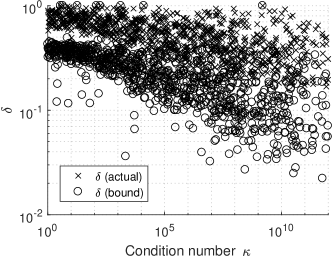
(a)

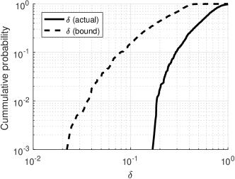
(b)

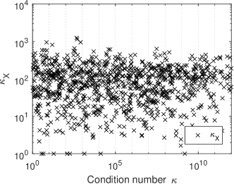
(c)

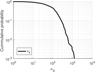
(d)

Figure 5: Statistics for $\delta$ and $\kappa_{X}$ for the 1000 randomly-generated problems in Fig. 1: (a) & (b) scatter plot and empirical CDF for $\delta$ and its lower bound $\delta_{\mathrm{lb}}$ (Lemma 5.5); (c) & (d) scatter plot and empirical CDF for $\kappa_{X}$.

Earlier in the introduction, we presented a comparison of ADMM and ADMM-GMRES for 1000 random trials. These problems were generated using the following algorithm.

Input: dimension parameters $n$, $\ell\leq n$, $m\leq\ell$ and conditioning parameter $s>0$.
Output: random data matrices $D\in\mathbb{S}^{n}$, $A\in\mathbb{R}^{\ell\times n}$, $B\in\mathbb{R}^{\ell\times m}$ satisfying Assumption 2.5.

1. Select the singular vectors $U_{A},U_{B},U_{D},V_{A},V_{B}$ i.i.d. uniformly from their respective orthogonal groups.

2. Select the singular values $\Sigma_{A},\Sigma_{B},\Sigma_{D}$ i.i.d. from the log-normal distribution $\sim\mathrm{exp}(0,s^{2})$.

3. Output $A=U_{A}\Sigma_{A}V_{A}^{T}$, $B=U_{B}\Sigma_{B}V_{B}^{T}$, and $D=U_{D}\Sigma_{D}U_{D}^{T}$.

More specifically, the dimension parameters $n,\ell,m$ were uniformly sampled from $n=1000$, $\ell\in\{1,\ldots,n\}$, and $m\in\{1,\ldots,\ell\}$, and the log-standard-deviation is swept within the range $s\in[0,2]$. Both algorithms are tasked with solving the equation to a relative residual of $\epsilon=10^{-6}$. ADMM fails to converge within 100,000 iterations for 49 of the problems, while ADMM-GMRES converges on all of the problems.

To verify whether Theorem 5.3 is sufficient to explain the $O(\kappa^{1/4})$ behavior seen in these 1000 random problems, we plot the distribution of $\delta$ and $\kappa_{X}$ with respect to $\kappa$ in Fig. 5a and Fig. 5c. The smallest value of $\delta$ is 0.06, with mean and median both around 0.6. The largest value of $\kappa_{X}$ is 775, with mean and median both around 50. These are both relatively modest, and as predicted by Theorem 5.3, ADMM-GMRES converges in $O(\kappa^{1/4})$ iterations.

The associated cumulative probability distributions are shown in Fig. 5b and Fig. 5d. An exponentially decaying probability tail for both quantities can be observed. The rapid roll-off in probability tail is a signature trait for concentration-of-measure type results. In the case of $\delta$, consider the following bound.

Lemma 5.5.

Define $K(\beta)$, $Q$, $P$ as in (3.4). Then

$$\delta_{\mathrm{lb}}\triangleq 1-\frac{\|Q^{T}K(\beta)Q\|+\|P^{T}K(\beta)P\|}{2\|K(\beta)\|}\leq\delta.$$

Proof 5.6.

Note that $K(\beta)$ has the following block structure $K=\left[\begin{smallmatrix}X&Z\\ -Z^{T}&Y\end{smallmatrix}\right]$. For such matrices, Benzi & Simoncini [12] used a field-of-values type argument to show that if $\lambda\in\Lambda\{K\}$ and $\mathrm{Im}\{\lambda\}\neq 0$, then $|\mathrm{Re}\lambda|\leq\frac{1}{2}\left[\|X\|+\|Y\|\right]$. Substituting the definitions of $\delta$, $X$, and $Y$ results in the desired bound.

Hence, we see that the quantity $\delta$ is bounded away from zero because the matrices $K$, $Q$, $P$ are incoherent. More specifically, let us write $K=U\Sigma V^{T}$ as its singular value decomposition. If we treat $Q$, $P$, $U$, and $V$ all as random orthogonal matrices, then the matrices $Q^{T}U$, $P^{T}U$, $Q^{T}V$, and $P^{T}V$ are all dense with an overwhelming probability [24, Thm.VIII.1]. This observation bounds the expected value of $\|Q^{T}K(\beta)Q\|$ and $\|P^{T}K(\beta)P\|$ away from $\|K(\beta)\|$, thereby bounding $\delta$ away from zero via Lemma 5.5.

6 The normality assumption

A weakness in our argument is Assumption 5, which takes $\kappa_{X}$, the condition number for the matrix of eigenvectors of $K(\beta)$, to be bounded. The assumption is closely related to the normality of $K(\beta)$. A matrix is normal if it has a complete set of orthogonal eigenvectors, so if $K(\beta)$ is normal, then $\kappa_{X}=1$, and our bounds are sharp up to a multiplicative factor. On the other hand, if $K(\beta)$ is nonnormal, then our bounds may fail to be sharp to an arbitrary degree. The phenomenon has to do with the fact that eigenvalues are not necessarily meaningful descriptors for the behavior of nonnormal matrices; see the discussions in [41, 25, 27] for more details, and the book [74] for a thorough exposition.

In the case of ADMM, there are reasons to believe that $K(\beta)$ is relatively close to normal, and that Assumption 5 is not too strong in practice. To explain, consider the following dimensionless nonnormality measure

$$\nu(A)\triangleq\|A^{T}A-AA^{T}\|_{F}^{1/2}/\|A\|_{F},$$

which takes on values from 0 (attained by any normal matrix) to $\sqrt{2}$ (attained by highly nonnormal matrices like $\left[\begin{smallmatrix}0&0\\ 1&0\end{smallmatrix}\right]$). The measure is closely associated to Henrici’s departure from normality [43], and can be used to bound many other measures of nonnormality; see the survey in [26].

Proposition 6.1.

Let $K(\beta)$ be the $\ell\times\ell$ matrix in (3.4). Then

$$\nu(K(\beta))\leq\frac{\left(8\min\{m,\ell-m\}\right)^{1/4}}{\|K(\beta)\|_{F}/\|K(\beta)\|}\leq\sqrt{2}\ell^{1/4}\frac{\|K(\beta)\|}{\|K(\beta)\|_{F}}.$$

Proof 6.2.

Note that $K\equiv K(\beta)$ has the structure $K=JU^{T}WU$, where $J=\mathrm{diag}\,(I_{m},-I_{\ell-m})$, $U$ is orthonormal, and $W=W^{T}$ shares its singular values with $K$. Then $\|K^{T}K-KK^{T}\|_{F}^{2}=\|UW^{2}U-JU^{T}W^{2}UJ\|_{F}^{2}=2\|2Q^{T}W^{2}P\|_{F}^{2}$, where $Q$ is the first $m$ columns of $U$, and $P$ is the remaining $\ell-m$ columns. But $\|Q^{T}W^{2}P\|_{F}^{2}=\mathrm{tr}\,W^{2}QQ^{T}W^{2}PP^{T}\leq\|W\|^{4}\min\{\mathrm{tr}\,QQ^{T},\mathrm{tr}\,PP^{T}\}$, and taking fourth roots produces the first inequality. The second inequality follows by maximizing the bound with $\ell=m/2$.

In the literature, the ratio $\|K\|_{F}^{2}/\|K\|^{2}$ is sometimes known as the numerical rank of $K$; see [65]. Taking on a value from $1$ to $\ell$, it is always bounded by, and is a stable relaxation of, the rank of $K$.

Assuming that the numerical rank of $K$ grows linearly with its dimension $\ell$ (e.g. if the data were generated using Algorithm 5.2), then substituting $\|K\|_{F}^{2}/\|K\|^{2}\in\Omega(\ell)$ into Proposition 6.1 produces $\nu(K)\in O(\ell^{-1/4})$. The matrix $K$ becomes more and more normal as its dimension $\ell$ grows large, since $\nu(K)$ decays to zero. While the observation does not provide a rigorous bound for $\kappa_{X}$, it does concur with our numerical results presented in later sections.

Finally, even if Assumption 5 fails to hold, ADMM-GMRES will still obey its worst-case bound (Proposition 4.3). Convergence is guaranteed in $O(\sqrt{\kappa})$ iterations, although the significant acceleration from GMRES may be lost.

7 Comparison with classical preconditioners

Throughout this paper, we have treated ADMM-GMRES as a preconditioned Krylov subspace method for the KKT equations associated with (ECQP)

(7.1) $$\left[\begin{array}[]{cc|c}D&0&A^{T}\\ 0&0&B^{T}\\ \hline\cr A&B&0\end{array}\right]\left[\begin{array}[]{c}x\\ z\\ \hline\cr y\end{array}\right]=\left[\begin{array}[]{c}-c\\ -p\\ \hline\cr d\end{array}\right],$$

while assuming that matrix-vector products with $(\beta^{-1}D+A^{T}A)^{-1}$, $(B^{T}B)^{-1}$, $A$, $B$, $A^{T}$ and $B^{T}$ can be efficiently performed, i.e. efficient oracles are available. But (7.1) is a standard saddle-point system—albeit with a singular $(1,1)$ block—and preconditioned Krylov subspace methods for such problems are mature and well-developed; we refer the reader to the authoritative surveys [11, 3]. A number of classical preconditioners can be constructed using these same oracles, many of them even sharing the same $O(\sqrt{\kappa})$ worst-case iteration bound as ADMM.

An important finding in this paper is that the average-case behavior of ADMM-GMRES is considerably better than its worst-case. In fact, our results from Section 5 suggest that the worst-case bound is almost never attained, except on artificially constructed “degenerate” problems. It is natural to ask whether the same thing can be said for the alternative preconditioners, which are constructed using the same ingredients. Will they also converge in $O(\kappa^{1/4})$ iterations? Or will they readily attain their worst-case bound of $O(\sqrt{\kappa})$ iterations?

In this section, we benchmark ADMM-GMRES against classical preconditioned Krylov subspace methods for saddle-point problems, on random instances of (7.1) generated using Algorithm 5.2. We restrict our attention to classical preconditioners that are based on the same six matrix-vector products listed above, and also matrix-vector products with $AD^{-1}A^{T}$ and its inverse $(AD^{-1}A^{T})^{-1}$, the former of which arises by block-eliminating $D$ from (7.1). Our goal is to compare the number of iterations needed by different preconditioners to solve the same $\kappa$-conditioned problem to $\epsilon$-accuracy.

A practical issue overlooked by a direct comparison of iteration counts (and the number of oracle calls) is that some oracles are considerably more expensive to call. To account for this, we use the CPU time as a weighted tally of oracle calls, by implementing the relative timings of the oracles proportional to their real-life values. To this end, we implement the matrix-vector products with $A,$ $B,$ $A^{T},$ and $B^{T}$ explicitly, and make the following assumption to reduce the cost of matrix-vector products with $(\beta^{-1}D+A^{T}A)^{-1},$ $(B^{T}B)^{-1},$ $AD^{-1}A^{T},$ and $(AD^{-1}A^{T})^{-1}$. The Cholesky factorizations $B^{T}B=L_{B}L_{B}^{T}$, $D=L_{D}L_{D}^{T}$, and the eigendecomposition $(AD^{-1}A^{T})^{-1}=V\Lambda V^{T}$ are explicitly available. Using Assumption 7, matrix-vector products with $(B^{T}B)^{-1}$ may be implemented as $z\mapsto L_{B}^{-T}L_{B}^{-1}z$, those with $AD^{-1}A^{T},$ $(AD^{-1}A^{T})^{-1}$ may be implemented as $y\mapsto V\Lambda^{-1}V^{T}y$ and $y\mapsto V\Lambda V^{T}y$, and those with $(\beta^{-1}D+A^{T}A)^{-1}$ may be implemented as

$$x\mapsto(\beta^{-1}D+A^{T}A)^{-1}x =\beta D^{-1}\left[I-A^{T}(\beta^{-1}I+AD^{-1}A^{T})^{-1}AD^{-1}\right]x.$$

The assumption is modeled after the Newton subproblem in Section 8, which satisfies it in near-linear time due to a Kronecker structure described in Section 8.1. It is slightly stronger that what is strictly necessary to realize the oracles for the comparison; we adopt it because it closely mimics the implementation considerations for Section 8.

7.1 Classical preconditioners

We restrict our attention to classical preconditioners that can be realized using only matrix-vector products with $(\beta^{-1}D+A^{T}A)^{-1},$ $(B^{T}B)^{-1},$ $A,$ $B,$ $A^{T},$ $B^{T}$, $AD^{-1}A^{T},$ and $(AD^{-1}A^{T})^{-1}$. These methods are selected from the survey [11], and solve either the reduced augmented system

(7.2) $$\left[\begin{array}[]{c|c}0&B^{T}\\ \hline\cr B&-AD^{-1}A^{T}\end{array}\right]\left[\begin{array}[]{c}z\\ \hline\cr y\end{array}\right]=\left[\begin{array}[]{c}-p\\ \hline\cr\tilde{d}\end{array}\right],$$

or the Schur complement problem

(7.3) $$\left[B^{T}(AD^{-1}A^{T})^{-1}B\right]z=-\tilde{p},$$

where the new right-hand sides are obtained via forward substitution

(7.4) $$\tilde{d}=d+AD^{-1}c,\qquad\tilde{p}=p-B^{T}(AD^{-1}A^{T})^{-1}\tilde{d},$$

and the unknown variables are recovered via back substitution

(7.5) $$y=(AD^{-1}A^{T})^{-1}(Bz-\tilde{d}),\qquad x=-D^{-1}(A^{T}y+c).$$

Note that each forward substitution (7.4), backward substitution (7.5), and matrix-vector product with (7.2) and (7.3) can be performed using only the 8 matrix-vector oracles listed above.

Block-diagonal preconditioner (Blk-Diag). Solve the reduced augmented system (7.2) using a symmetric indefinite Krylov method like MINRES, with the positive definite matrix

$$M_{1}=\left[\begin{array}[]{c|c}\beta B^{T}B&0\\ \hline\cr 0&AD^{-1}A^{T}\end{array}\right]$$

serving as preconditioner. The $(2,2)$ block of $M_{1}$ matches that of $\hat{H}$, while its $(1,1)$ block is used to precondition the Schur complement. The preconditioned matrix has the eigenvalue $-1$ with multiplicity $m-\ell$, and $2\ell$ eigenvalues $\lambda_{i}=\frac{1}{2}(-1\pm\sqrt{1+4\eta_{i}})$, where $\eta_{1},\ldots,\eta_{\ell}$ are the $\ell$ eigenvalues of $\beta^{-1}Q^{T}\tilde{D}Q$ [30, Lem.2.1] (see also [11, Thm.3.8] and [66, Lem.2.1]). Applying the classic two-interval approximation result [22] (see also [41, Ch.3]) shows that MINRES converges to an $\epsilon$-accurate solution within $k\leq 1+\left\lceil\sqrt{\kappa}\log[(1+\sqrt{1+4L/\beta})/\epsilon]\right\rceil$ iterations. We set $\beta=L$ to obtain convergence in $O(\sqrt{\kappa})$ iterations.

Constraint preconditioner I (Constr I). Solve the reduced augmented system (7.2) using a general Krylov method like GMRES, with

$$M_{2}=\left[\begin{array}[]{c|c}0&B^{T}\\ \hline\cr B&-\beta I\end{array}\right]=\left[\begin{array}[]{c|c}I&\beta^{-1}B^{T}\\ \hline\cr 0&I\end{array}\right]\left[\begin{array}[]{c|c}\beta^{-1}B^{T}B&0\\ \hline\cr 0&-\beta I\end{array}\right]\left[\begin{array}[]{c|c}I&0\\ \hline\cr\beta^{-1}B&I\end{array}\right]$$

serving as preconditioner. The preconditioner is designed to replicate the governing matrix, while modifying the $(2,2)$ block in a way as to make the overall matrix considerably easier to invert. The preconditioned matrix has the eigenvalue 1 with multiplicity $2\ell$, and $m-\ell$ eigenvalues that coincide with the eigenvalues of $\beta^{-1}P^{T}\tilde{D}^{-1}P$ [47, Thm.2.1]; see also [11, Thm.10.1]. The latter $m-\ell$ eigenvalues lie within the real interval $[1/(L\beta),1/(\mu\beta)]$, so assuming diagonalizability (i.e. adopting a version of Assumption 5), GMRES converges within $O(\sqrt{\kappa})$ iterations for all choices of $\beta\geq 1/L$. We set $\beta=\sqrt{\mu L}$ to concur with ADMM.

Constraint preconditioner II (Constr II). Solve the Schur complement system (7.3) using a symmetric positive definite Krylov method like conjugate residuals, with

$$M_{3}=B^{T}B$$

serving as preconditioner. This is derived by using the Schur complement from the previous preconditioner to precondition the Schur complement of (7.2). The preconditioned problem has coefficient matrix $Q^{T}\tilde{D}Q,$ whose eigenvalues lie in the real interval $[\mu,L]$. Accordingly, conjugate residuals converges within $O(\sqrt{\kappa})$ iterations.

Hermitian Skew-Hermitian Splitting (HSS). Solve the reduced augmented system (7.2) using a general Krylov method like GMRES, with

$$M_{4}=\left[\begin{array}[]{c|c}\alpha I&0\\ \hline\cr 0&-(AD^{-1}A^{T}+\alpha I)\end{array}\right]\left[\begin{array}[]{c|c}\alpha I&B^{T}\\ \hline\cr-B&\alpha I\end{array}\right]$$

as preconditioner. Small choices of the parameter $\alpha$ work best, though the method is not sensitive to its exact value [9, 10, 70]. Note that $M_{4}$ requires matrix-vector products with $(\alpha^{2}I+B^{T}B)^{-1}$ to be efficient. When $\alpha$ is sufficiently small, this matrix may be approximated, e.g. using a few iteration of conjugate gradients preconditioned by $B^{T}B$. To keep our implementation simple, we set $\alpha=1/L$ (as recommended by Simoncini and Benzi [70]) and explicitly precompute a Cholesky factorization for $\alpha^{2}I+B^{T}B$.

Our list excludes the Uzawa method (and its inexact variants), incomplete factorizations, and multilevel / hierarchical preconditioners, because they cannot be efficiently realized using the 8 matrix-vector oracles alone. We have excluded the Arrow–Hurwicz as it is simply a lower-cost, less accurate version of “Constr I”. We have also excluded the block-triangular version of “Blk-Diag”, because it can be shown to be almost identical to “Constr II” after a single iteration, but requires the more computationally expensive GMRES algorithm.

7.2 Results

Table 1: Max. Iterations (Max. CPU time in seconds) to $\epsilon=10^{-6}$ for random problems with dimensions $n=1000$, $1\leq m\leq n$, $1\leq\ell\leq m$. “ADGM” refers to ADMM-GMRES, and “ADGM($k$)” refers to ADMM-GMRES($k$), i.e. with restart parameter $k$.

$\log_{10}\kappa$	$(0,2]$	$(2,4]$	$(4,6]$	$(6,8]$	$(8,10]$
Num. trials	204	192	169	185	135
$10\sqrt{\kappa}$	32	316	3162	31,623	316,228
ADMM	126 (0.97)	982 (5.09)	$>10^{3}$	$>10^{3}$	$>10^{3}$
Blk-Diag	102 (0.52)	506 (3.27)	$>10^{3}$	$>10^{3}$	$>10^{3}$
Constr I	42 (0.45)	155 (1.19)	269 (2.11)	553 (3.10)	678 (4.43)
Constr II	49 (0.19)	227 (1.28)	722 (3.00)	$>10^{3}$	$>10^{3}$
HSS	97 (2.72)	278 (12.6)	532 (19.4)	$>10^{3}$	$>10^{3}$
$6\kappa^{1/4}$	11	34	107	337	1067
ADGM	13 (0.23)	29 (0.55)	76 (1.24)	198 (3.94)	469 (6.44)
ADGM(5)	14 (0.25)	50 (0.68)	$>10^{3}$	$>10^{3}$	$>10^{3}$
ADGM(10)	13 (0.21)	37 (0.51)	$>10^{3}$	$>10^{3}$	$>10^{3}$
ADGM(25)	13 (0.20)	30 (0.50)	$>10^{3}$	$>10^{3}$	$>10^{3}$

Table 2: Max. Iterations (Max. CPU time in seconds) to $\epsilon=10^{-6}$ for random problems with dimensions $n=3000$, $1\leq m\leq n$, $1\leq\ell\leq m$.

$\log_{10}\kappa$	$(0,2]$	$(2,4]$	$(4,6]$	$(6,8]$	$(8,10]$
Num. trials	242	236	210	195	110
$10\sqrt{\kappa}$	32	316	3162	31,623	316,228
ADMM	85 (9.87)	910 (98.8)	$>10^{3}$	$>10^{3}$	$>10^{3}$
Blk-Diag	96 (4.14)	568 (20.2)	$>10^{3}$	$>10^{3}$	$>10^{3}$
Constr I	52 (3.75)	244 (10.8)	636 (20.5)	$>10^{3}$	$>10^{3}$
Constr II	46 (1.65)	254 (8.18)	$>10^{3}$	$>10^{3}$	$>10^{3}$
HSS	87 (19.8)	378 (72.8)	843 (212)	$>10^{3}$	$>10^{3}$
$6\kappa^{1/4}$	11	34	107	337	1067
ADGM	12 (1.36)	28 (4.01)	116 (7.77)	199 (23.15)	431 (69.54)
ADGM(5)	13 (1.65)	45 (5.98)	$>10^{3}$	$>10^{3}$	$>10^{3}$
ADGM(10)	12 (1.28)	37 (4.07)	$>10^{3}$	$>10^{3}$	$>10^{3}$
ADGM(25)	12 (1.37)	30 (4.61)	$>10^{3}$	$>10^{3}$	$>10^{3}$

Table 3: Associated max. initial set-up CPU time in seconds

	Factoring	Factoring	Forming and eigendecomposing
$n$	$B^{T}B=L_{B}L_{B}^{T}$	$D=L_{D}L_{D}^{T}$	$AD^{-1}A^{T}=V\Lambda^{-1}V^{T}$
1000	0.0658	0.0325	0.3610
3000	1.1122	0.4802	7.0947

We solved 1000 random problems with $n=1000$, $1\leq m\leq n$, $1\leq\ell\leq m$, and 1000 random problems with $n=3000$, $1\leq m\leq n$, $1\leq\ell\leq m$, using ADMM, ADMM-GMRES, and the four preconditioned Krylov methods described above, on an Intel Core i7-3960X CPU with six 3.30 GHz cores. All six methods were set to terminate at 1000 iterations. Accuracy was measured as the relative residual norm with respect to the saddle-point equation (7.1).

Tables 3 & 3 show the number of iterations and CPU time to $10^{-6}$ accuracy. Table 3 shows the associated set-up times for the three oracles in Assumption 7. ADMM and all four of the preconditioner Krylov methods converge in $O(\sqrt{\kappa})$ iterations, but ADMM-GMRES consistently converges in $O(\kappa^{1/4})$ iterations. This square-root factor acceleration is large enough to offset the high per-iteration cost of the method in every case. However, note that the preconditioner “Constr I” does not require access to the eigendecomposition of $AD^{-1}A^{T}$, and so enjoys a considerable set-up time advantage over ADMM-GMRES. Once the condition number exceeds $\kappa\geq 10^{4}$, the square-root acceleration becomes large enough to offset the fairly hefty cost of computing the eigendecomposition, making it the fastest overall. The restarted GMRES variant enjoys some of this acceleration, but is also susceptible to stalling once the problem becomes sufficiently ill-conditioned.

The constraint preconditioner “Constr I” performs surprisingly well for the $n=1000$ examples in Table 3, consistently outperforming its $O(\sqrt{\kappa})$ iteration bound. Examining closer, however, we find this to be an artifact of the finite convergence property of GMRES. Once the problem size is increased to $n=3000$, the method is no longer able to solve ill-conditioned problems with $\kappa\geq 10^{6}$.

In all of these examples, the per-iteration costs remain approximately constant—even for methods that relied on GMRES—due to the relatively high cost of the preconditioners. Profiling the code, we find that each GMRES iteration takes no more than 4 milliseconds to execute. By contrast, even our fastest preconditioner (Constr II) requires $\sim 36$ milliseconds per application.

8 Solving the SDP Newton subproblem

Now, we consider using ADMM-GMRES to solve the Newton subproblem associated with an interior-point solution of the semidefinite program in (SDP). Recall from Section 1.4 that the Newton subproblem solved at each interior-point iteration has the general form

(8.1) minimize $$\frac{1}{2}\|W^{1/2}(X-\hat{X})W^{1/2}\|_{F}^{2}+p^{T}z$$

subject to $$X+\sum_{i=1}^{m}z_{i}B_{i}=Q,$$

in which all matrices are $\theta\times\theta$ real symmetric. The symmetric positive definite matrix $W$ is known as the scaling matrix, and is generally fully-dense. Different interior-point methods differ in how the scaling matrix $W$ is constructed, but in every case, the matrix becomes progressively ill-conditioned as the interior-point method makes progress towards the solution. To be specific, the matrix $W$ has a condition number $\mathrm{cond}(W)=\Theta(1/\epsilon)$ at an interior-point iterate with duality gap $\epsilon$, and this gives (8.1) the condition number of $\kappa=\Theta(1/\epsilon^{2})$; see [80] and also [73, 72]. We must solve this highly ill-conditioned problem to a similar level of accuracy as the current duality gap $\epsilon$ in order for further progress to be made.

Indeed, (8.1) is just an instance of (ECQP). To see this, we define the vectorization $\mathrm{vec}\,X$ of a given $\theta\times\theta$ matrix $X$ as the size-$\theta^{2}$ column vector made up of sequential columns of $X$ stacked on top of each other, and the Kronecker product $A\otimes B$ implicitly to satisfy the Kronecker identity $(A\otimes B)\mathrm{vec}\,X=\mathrm{vec}\,(BXA^{T})$. Using these two operations, we can rewrite (8.1) as

(8.2) minimize $$\frac{1}{2}x^{T}(W\otimes W)x+c^{T}x+p^{T}z$$

subject to $$x+Bz=q,$$

where $x=\mathrm{vec}\,X,$ $c=-\mathrm{vec}\,(W\hat{X}W),$ $B=[\mathrm{vec}\,B_{1},\ldots,\mathrm{vec}\,B_{m}]$, and $q=\mathrm{vec}\,Q$. This is an instance of (ECQP), over the variables $x\in\mathbb{R}^{n}$ of dimension $n=\theta^{2}$ and $z\in\mathbb{R}^{m}$ of dimension $m$, and subject to $\ell=n=\theta^{2}$ equality constraints. Note that $B$ must have full column-rank in order for the associated SDP to be nondegenerate [1], so we must always have $m\leq n$.

Standard interior-point methods solve (8.2) directly by forming and factoring (the Schur complement of) its KKT equations, in cubic $O(n^{3/2}m+nm^{2}+m^{3})$ time and quadratic $\Theta(m^{2})$ memory. The goal of this section is solve (8.2) at reduced cost using ADMM and ADMM-GMRES. In Section 8.1 below, we explain how each iteration of ADMM can be performed in as low as $O(n^{3/2}+m)$ time and $O(n+m)$ memory. Then, in Sections 8.2 and 8.3, we show that ADMM-GMRES solves the Newton subproblems associated with an interior-point solution of the SDPLIB [14] and DIMACS [62] benchmark problems to $\epsilon$-accuracy in $O(\kappa^{1/4}\log\epsilon^{-1})$ iterations.

8.1 Implementation

We begin by noting that the $n\times n$ dense matrix $W\otimes W$ can be diagonalized in $O(n^{3/2}$) time and $O(n)$ memory. This arises from the fact that $(A\otimes B)(C\otimes D)=AC\otimes BD$. Once we have an eigendecomposition for the $\theta\times\theta$ matrix $W=V\Lambda V^{T}$ in $O(\theta^{3})$ time and $O(\theta^{2})$ memory, we immediately have an eigendecomposition for the $\theta^{2}\times\theta^{2}$ matrix $W\otimes W=(V\otimes V)(\Lambda\otimes\Lambda)(V\otimes V)^{T}$. This insight gives us explicit values for the Lipschitz constant $L=\lambda_{\max}(W\otimes W)=\lambda_{\max}^{2}(W)$ and the strong convexity constant $\mu=\lambda_{\min}(W\otimes W)=\lambda_{\min}^{2}(W)$, and shows that $\kappa=L/\mu=\mathrm{cond}(W)^{2}=\Theta(1/\epsilon^{2})$.

Now, we apply ADMM to (8.2), and obtain the following iterations

(8.3a) $$x^{k+1} =(\beta^{-1}W\otimes W+I)^{-1}(c+q-Bz^{k}-y^{k})$$

(8.3b) $$z^{k+1} =(B^{T}B)^{-1}[\beta^{-1}p-B^{T}(x^{k+1}+y^{k}-q)]$$

(8.3c) $$y^{k+1} =y^{k}+(x^{k+1}+Bz^{k+1}-q).$$

After computing the eigendecomposition $W=V\Lambda V^{T}$, we set the algorithm parameter $\beta$ to $\sqrt{\mu L}=\lambda_{\max}(W)\lambda_{\min}(W)$, in order to for the sequence to converge in $O(\sqrt{\kappa})$ iterations.

Each iteration requires a single matrix-vector product with $(\beta^{-1}W\otimes W+I)^{-1},$ $B,$ $B^{T}$, and $(B^{T}B)^{-1}$. The first matrix-vector product $\mathrm{vec}\,X=(\beta^{-1}W\otimes W+I)^{-1}\mathrm{vec}\,Y$ can be efficiently implemented in $O(n^{3/2})$ time and $O(n)$ memory using the eigendecomposition $W=V\Lambda V^{T}$ and the following formula

$$X=V\left(\left[\frac{1}{\beta^{-1}\lambda_{i}\lambda_{j}+1}\right]_{i,j=1}^{\theta}\circ(V^{T}YV)\right)V^{T},$$

obtained by diagonalizing $(\beta^{-1}W\otimes W+I)=(V\otimes V)(\beta^{-1}\Lambda\otimes\Lambda+I)(V\otimes V)^{T}$. Here, $\circ$ denotes the element-wise Hadamard product.

The cost of matrix-vector products with $B$, $B^{T}$, $(B^{T}B)^{-1}$, however, depends on the sparsity of the SDP to be solved. For many SDPs, particularly those that arise from combinatorial problems, the matrix $B$ is highly sparse, and the matrix $B^{T}B$ admits a sparse Cholesky factorization, so all three operations can be performed in linear $O(m)$ time. However, for other problems, $B^{T}B$ may suffer from catastrophic fill-in, and in this case, the matrix-vector product $(B^{T}B)^{-1}$ may require up to cubic $O(m^{3})$ time and quadratic $O(m^{2})$ memory to implement. This issue of factoring $B^{T}B$ is common to all ADMM-based approaches to SDPs; see [79, Rem.2], [59, Sec.4] and the references therein. In some cases, an iterative method like conjugate gradients may be used [15, Ch.4], possibly alongside an incomplete factorization preconditioner, though this can greatly increase the per-iteration cost, thereby diminishing the appeal of ADMM.

8.2 The SDPLIB problems

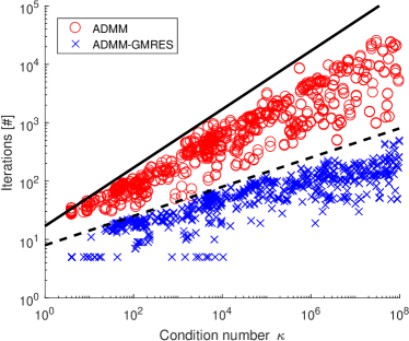
(a)

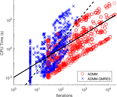
(b)

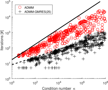
(c)

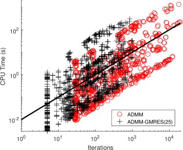
(d)

Figure 6: Iterations to $\epsilon=10^{-6}$ residual convergence for the 1038 Newton direction problems described in-text: (a) & (b) ADMM vs ADMM-GMRES; (c) & (d) ADMM vs ADMM-GMRES(25)

We generate instances of (8.2) using SeDuMi [71] over the 80 problems in the SDPLIB suite [14] with $m\leq 700$. This collection encompasses a diversity of practical semidefinite programs, and $m$ is small enough so that the matrix $B^{T}B$ may always be inverted at a reasonable cost. At the same time, the iterates $u^{k}$ have dimensions up to $n+\ell+m\leq 789264$ (for the problem truss8), which is large enough for the comparisons to be realistic. For each problem, the predictor and corrector Newton subproblems with $\kappa\leq 10^{8}$ are extracted and solved using ADMM and ADMM-GMRES on an Intel Xeon E5-2687W CPU with eight 3.10 GHz cores. The stopping condition is set to be $10^{-6}$ relative residual, i.e. when an iterate $u^{k}$ is found such that $\|u^{k}-u^{\star}\|_{M}/\|u^{\star}\|_{M}\leq 10^{-6}$. The maximum number of iterations for both methods is capped at 1000.

Fig. 6a shows the number of iterations to convergence. Results validate the $O(\sqrt{\kappa})$ figure expected of ADMM, and the $O(\kappa^{1/4})$ figure expected of GMRES. In fact, the multiplicative constants associated with each appear to be very similar to the results shown earlier in Fig. 1. Fig. 6b compares the associated CPU times with the number of iterations. The per-iteration cost of ADMM-GMRES is constant for small $k$, but grows linearly with $k$ beyond about 30 iterations. For many of the problems considered, the square-root factor reduction in iterations to convergence is offset by the quadratic growth in computation time, and both methods end up using a similar amount of time, despite the considerable difference in iteration count.

A practical implementation of ADMM-GMRES will require the use of a limited-memory version of GMRES. We consider the simplest approach of restarting every 25 iterations; the results are shown in Figs. 6c & 6d. The restarted variant requires a factor of two more iterations to converge when compared to the usual algorithm. The amortized per-iteration cost of restarted ADMM-GMRES is a factor of two times higher that of basic ADMM, but the method also converges in significantly fewer iterations.

8.3 The DIMACS problems

Table 4: Solving DIMACS Problems using SeDuMi modified to compute search directions using ADMM-GMRES(25). “CPU” is total CPU time in seconds, “Iter” is the total inner ADMM-GMRES iterations taken, and “feas” and “opt” are defined in-text.

Key	Name	$m$	$\theta$	$N$	CPU	Iter	feas	opt
a	hamming_7_5_6	1793	128	$3.46\times 10^{4}$	2.86	300	6.59	7.92
b	hamming_8_3_4	16129	256	$1.47\times 10^{5}$	11.5	347	6.37	8.16
c	hamming_9_5_6	53761	512	$5.78\times 10^{5}$	85.2	422	6.45	7.89
d	hamming_9_8	2305	512	$5.27\times 10^{5}$	70.4	411	5.39	7.47
e	hamming_10_2	23041	1024	$2.12\times 10^{6}$	256	328	5.40	7.94
f	hamming_11_2	56321	2048	$8.44\times 10^{6}$	1262	217	3.98	6.36
g	toruspm3-8-50	512	512	$5.25\times 10^{5}$	201	1651	2.53	4.91
h	torusg3-8	512	512	$5.25\times 10^{5}$	950	8906	3.64	6.07
i	torusg3-15	3375	3375	$2.28\times 10^{7}$	26721	3280	1.68	4.88
j	toruspm3-15-50	3375	3375	$2.28\times 10^{7}$	36782	4387	2.20	5.42

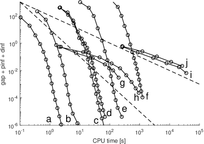
(a)

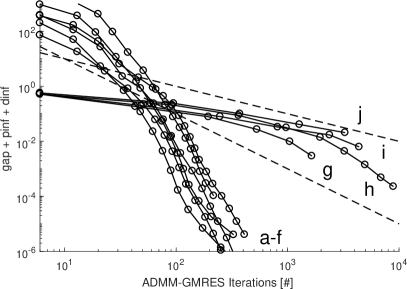
(b)

Figure 7: The convergence behavior of embedding ADMM-GMRES within SeDuMi for the DIMACS problems: (a) against CPU time; (b) against inner ADMM-GMRES iterations. Data for the keys are shown in Table 4. Each marker shows a single interior-point iteration. The dash lines indicate sublinear $O(1/k)$ and $O(1/k^{2})$ error rates.

Finally, we incorporate ADMM-GMRES within SeDuMi, as a set of inner iterations within an outer interior-point method, in order to solve large-scale SDPs from the Seventh DIMACS Implementation Challenge [62]. In other words, we modify SeDuMi to use ADMM-GMRES to compute the Newton search directions, in lieu of its internal Cholesky-based solver, while leaving the remainder of the solver unchanged. The Newton subproblems are large enough to prevent the full GMRES from being used, so we restart GMRES every 25 iterations, allowing up to 1000 inner iterations to be performed per outer interior-point iteration. The inner ADMM-GMRES iterations are terminated when an iterate $u^{k}$ is found such that $\|H(u^{k}-u^{\star})\|_{\infty}\leq\tau$, where $H$ is the KKT matrix for (8.2), and $\tau$ is an absolute tolerance as specified by the SeDuMi algorithm. Typically, $\tau$ is around one order of magnitude smaller than the current duality gap $\epsilon$. The outer interior-point iterations are terminated either by converging to the desired solution accuracy, or prematurely if SeDuMi considers the computed search direction to be too inaccurate to make further progress.

The numerical experiments are performed on an Intel Xeon E5-2609 v4 CPU with eight 1.70 GHz cores. Table 4 shows the results, and Fig. 7 plots the progress of the interior-point iterates over different interior-point iterations against time and against inner ADMM-GMRES iterations. Here, $N=n+\ell+m=2\theta^{2}+m$ refers to the total number of primal-dual variables in the corresponding (ECQP) problem. The accuracy of each interior-point iterate $\{X,y,S\}$ is quantified by the number of decimal digits of feasibility $\mathrm{feas}=-\log_{10}(\mathrm{pinf}+\mathrm{dinf})$ and digits of optimality $\mathrm{opt}=-\log_{10}(\mathrm{gap}),$ which are themselves defined in terms of the dimensionless DIMACS metrics [62]:

$$\mathrm{pinf}=\frac{\sqrt{\sum_{i}(\mathrm{tr}\,B_{i}Y-p_{i})^{2}}}{1+\|p\|_{2}},\qquad\mathrm{dinf}=\frac{\|\sum z_{i}B_{i}+X-Q\|_{F}}{1+\|Q\|_{F}}.$$

$$\mathrm{gap}=\frac{|\mathrm{tr}\,QY-p^{T}z|}{1+|\mathrm{tr}\,QY|+|p^{T}z|}.$$

The results show that ADMM-GMRES with restarts is able to converge within $O(\kappa^{1/4})$ iterations for 8 out of the 10 problems, namely the problems labeled from “a” to “h”. Their corresponding convergence curves demonstrate a time complexity of $O(1/\sqrt{\epsilon})$ and an error rate of $O(1/k^{2})$ at the $k$-th iteration. This is the “accelerated” rate that we described earlier in Section 1.4, typically obtained by “fast” first-order methods. For the remaining 2 problems, however, the method only converges in $O(\sqrt{\kappa})$ iterations, with a time complexity of $O(1/\epsilon)$ and an error rate of $O(1/k)$ at the $k$-th iteration. This is the usual rate attained by solving the interior-point Newton subproblem using a standard iterative method like conjugate gradients.

9 Conclusions and future work

In this paper, we have provided theoretical and numerical evidence that ADMM-GMRES can consistently converge in $O(\kappa^{1/4})$ iterations for a smooth strongly convex quadratic objective, despite a worst-case bound of $O(\sqrt{\kappa})$ iterations. The order-of-magnitude reduction in iterations over the basic ADMM method was widely observed for both randomized examples and in the Newton subproblems for the interior-point solution of semidefinite programs. These results confirm the possibility for an over-relaxation scheme, momentum scheme, or otherwise, to significantly accelerate the convergence of ADMM, beyond the constant factor typically observed for existing schemes, and suggest the direct use of ADMM-GMRES as a practical solution method.

It remains an open question whether the same sort of acceleration can be extended to ADMM for general nonquadratic objectives. One possible approach is to use GMRES to a linearized approximation of the nonlinear fixed-point equation, in a Krylov-Newton method [17]. Alternatively, a Broyden-like secant approximation may be constructed from previous iterates, and used to extrapolate the current step, in an Anderson acceleration method [78]. Both approaches reduce to ADMM-GMRES in the case of quadratic objectives, but further work is needed to understand their effectiveness.

References

- [1] F. Alizadeh, J.-P. A. Haeberly, and M. L. Overton, Complementarity and nondegeneracy in semidefinite programming, Mathematical Programming, 77 (1997), pp. 111–128.
- [2] M. S. Andersen, J. Dahl, and L. Vandenberghe, Logarithmic barriers for sparse matrix cones, Optimization Methods and Software, 28 (2013), pp. 396–423.
- [3] O. Axelsson, Unified analysis of preconditioning methods for saddle point matrices, Numerical Linear Algebra with Applications, 22 (2015), pp. 233–253.
- [4] A. Beck and M. Teboulle, A fast iterative shrinkage-thresholding algorithm for linear inverse problems, SIAM journal on imaging sciences, 2 (2009), pp. 183–202.
- [5] S. Becker, J. Bobin, and E. J. Candès, Nesta: A fast and accurate first-order method for sparse recovery, SIAM Journal on Imaging Sciences, 4 (2011), pp. 1–39.
- [6] S. Bellavia, J. Gondzio, and B. Morini, A matrix-free preconditioner for sparse symmetric positive definite systems and least-squares problems, SIAM Journal on Scientific Computing, 35 (2013), pp. A192–A211.
- [7] S. Bellavia, J. Gondzio, and M. Porcelli, An inexact dual logarithmic barrier method for solving sparse semidefinite programs, Mathematical Programming, (2018).
- [8] S. J. Benson, Y. Ye, and X. Zhang, Solving large-scale sparse semidefinite programs for combinatorial optimization, SIAM Journal on Optimization, 10 (2000), pp. 443–461.
- [9] M. Benzi, M. J. Gander, and G. H. Golub, Optimization of the Hermitian and skew-Hermitian splitting iteration for saddle-point problems, BIT Numerical Mathematics, 43 (2003), pp. 881–900.
- [10] M. Benzi and G. H. Golub, A preconditioner for generalized saddle point problems, SIAM Journal on Matrix Analysis and Applications, 26 (2004), pp. 20–41.
- [11] M. Benzi, G. H. Golub, and J. Liesen, Numerical solution of saddle point problems, Acta numerica, 14 (2005), pp. 1–137.
- [12] M. Benzi and V. Simoncini, On the eigenvalues of a class of saddle point matrices, Numerische Mathematik, 103 (2006), pp. 173–196.
- [13] L. Bergamaschi, J. Gondzio, and G. Zilli, Preconditioning indefinite systems in interior point methods for optimization, Computational Optimization and Applications, 28 (2004), pp. 149–171.
- [14] B. Borchers, SDPLIB 1.2, a library of semidefinite programming test problems, Optimization Methods and Software, 11 (1999), pp. 683–690.
- [15] S. Boyd, N. Parikh, E. Chu, B. Peleato, and J. Eckstein, Distributed optimization and statistical learning via the alternating direction method of multipliers, Foundations and Trends® in Machine Learning, 3 (2011), pp. 1–122.
- [16] J. H. Bramble and J. E. Pasciak, A preconditioning technique for indefinite systems resulting from mixed approximations of elliptic problems, Mathematics of Computation, 50 (1988), pp. 1–17.
- [17] P. N. Brown and Y. Saad, Convergence theory of nonlinear Newton–Krylov algorithms, SIAM Journal on Optimization, 4 (1994), pp. 297–330.
- [18] E. Candes and J. Romberg, l1-magic: Recovery of sparse signals via convex programming, URL: www.acm.caltech.edu/l1magic/, (2005).
- [19] A. Chambolle and T. Pock, A first-order primal-dual algorithm for convex problems with applications to imaging, Journal of mathematical imaging and vision, 40 (2011), pp. 120–145.
- [20] J. Dahl, L. Vandenberghe, and V. Roychowdhury, Covariance selection for nonchordal graphs via chordal embedding, Optimization Methods & Software, 23 (2008), pp. 501–520.
- [21] D. Davis and W. Yin, Faster convergence rates of relaxed Peaceman-Rachford and ADMM under regularity assumptions, arXiv preprint arXiv:1407.5210, (2014).
- [22] C. De Boor and J. R. Rice, Extremal polynomials with application to Richardson iteration for indefinite linear systems, SIAM Journal on Scientific and Statistical Computing, 3 (1982), pp. 47–57.
- [23] W. Deng and W. Yin, On the global and linear convergence of the generalized alternating direction method of multipliers, Journal of Scientific Computing, (2012), pp. 1–28.
- [24] D. L. Donoho and X. Huo, Uncertainty principles and ideal atomic decomposition, Information Theory, IEEE Transactions on, 47 (2001), pp. 2845–2862.
- [25] T. A. Driscoll, K.-C. Toh, and L. N. Trefethen, From potential theory to matrix iterations in six steps, SIAM review, 40 (1998), pp. 547–578.
- [26] L. Elsner and M. Paardekooper, On measures of nonnormality of matrices, Linear Algebra and its Applications, 92 (1987), pp. 107–123.
- [27] M. Embree, How descriptive are GMRES convergence bounds?, (1999).
- [28] E. Esser, X. Zhang, and T. F. Chan, A general framework for a class of first order primal-dual algorithms for convex optimization in imaging science, SIAM Journal on Imaging Sciences, 3 (2010), pp. 1015–1046.
- [29] V. Faber and T. Manteuffel, Necessary and sufficient conditions for the existence of a conjugate gradient method, SIAM Journal on Numerical Analysis, 21 (1984), pp. 352–362.
- [30] B. Fischer, A. Ramage, D. J. Silvester, and A. J. Wathen, Minimum residual methods for augmented systems, BIT Numerical Mathematics, 38 (1998), pp. 527–543.
- [31] M. Fortin and R. Glowinski, Augmented Lagrangian methods, (1983).
- [32] M. Fukuda, M. Kojima, K. Murota, and K. Nakata, Exploiting sparsity in semidefinite programming via matrix completion I: General framework, SIAM J. Optim., 11 (2001), pp. 647–674.
- [33] D. Gabay, Applications of the method of multipliers to variational inequalities, North-Holland, Amsterdam, 1983.
- [34] D. Gabay and B. Mercier, A dual algorithm for the solution of nonlinear variational problems via finite element approximation, Computers & Mathematics with Applications, 2 (1976), pp. 17–40.
- [35] E. Ghadimi, A. Teixeira, I. Shames, and M. Johansson, Optimal parameter selection for the alternating direction method of multipliers (ADMM): quadratic problems, Automatic Control, IEEE Transactions on, 60 (2015), pp. 644–658.
- [36] P. Giselsson and S. Boyd, Diagonal scaling in Douglas-Rachford splitting and ADMM, in Decision and Control (CDC), 2014 IEEE 53rd Annual Conference on, IEEE, 2014, pp. 5033–5039.
- [37] R. Glowinski and A. Marroco, Sur l’approximation, par éléments finis d’ordre un, et la résolution, par pénalisation-dualité d’une classe de problèmes de Dirichlet non linéaires, Revue française d’automatique, informatique, recherche opérationnelle. Analyse numérique, 9 (1975), pp. 41–76.
- [38] T. Goldstein, B. O’Donoghue, S. Setzer, and R. Baraniuk, Fast alternating direction optimization methods, SIAM Journal on Imaging Sciences, 7 (2014), pp. 1588–1623.
- [39] G. H. Golub and C. Greif, On solving block-structured indefinite linear systems, SIAM Journal on Scientific Computing, 24 (2003), pp. 2076–2092.
- [40] J. Gondzio, Matrix-free interior point method, Computational Optimization and Applications, 51 (2012), pp. 457–480.
- [41] A. Greenbaum, Iterative methods for solving linear systems, vol. 17, Siam, 1997.
- [42] B. He and X. Yuan, On the o(1/n) convergence rate of the Douglas-Rachford alternating direction method, SIAM Journal on Numerical Analysis, 50 (2012), pp. 700–709.
- [43] P. Henrici, Bounds for iterates, inverses, spectral variation and fields of values of non-normal matrices, Numerische Mathematik, 4 (1962), pp. 24–40.
- [44] M. Kadkhodaie, K. Christakopoulou, M. Sanjabi, and A. Banerjee, Accelerated alternating direction method of multipliers, in Proceedings of the 21th ACM SIGKDD International Conference on Knowledge Discovery and Data Mining, ACM, 2015, pp. 497–506.
- [45] A. Kalbat and J. Lavaei, A fast distributed algorithm for decomposable semidefinite programs, in Decision and Control (CDC), 2015 IEEE 54th Annual Conference on, IEEE, 2015, pp. 1742–1749.
- [46] N. Karmarkar, A new polynomial-time algorithm for linear programming, in Proceedings of the sixteenth annual ACM symposium on Theory of computing, ACM, 1984, pp. 302–311.
- [47] C. Keller, N. I. Gould, and A. J. Wathen, Constraint preconditioning for indefinite linear systems, SIAM Journal on Matrix Analysis and Applications, 21 (2000), pp. 1300–1317.
- [48] C.-J. Lin and J. J. Moré, Incomplete cholesky factorizations with limited memory, SIAM Journal on Scientific Computing, 21 (1999), pp. 24–45.
- [49] R. Madani, A. Kalbat, and J. Lavaei, ADMM for sparse semidefinite programming with applications to optimal power flow problem, in Decision and Control (CDC), 2015 IEEE 54th Annual Conference on, IEEE, 2015, pp. 5932–5939.
- [50] J. E. Mitchell, P. M. Pardalos, and M. G. Resende, Interior point methods for combinatorial optimization, in Handbook of combinatorial optimization, Springer, 1998, pp. 189–297.
- [51] N. M. Nachtigal, L. Reichel, and L. N. Trefethen, A hybrid GMRES algorithm for nonsymmetric linear systems, SIAM Journal on Matrix Analysis and Applications, 13 (1992), pp. 796–825.
- [52] K. Nakata, K. Fujisawa, M. Fukuda, M. Kojima, and K. Murota, Exploiting sparsity in semidefinite programming via matrix completion II: Implementation and numerical results, Math. Program., 95 (2003), pp. 303–327.
- [53] A. Nemirovskii, D. B. Yudin, and E. R. Dawson, Problem complexity and method efficiency in optimization, Wiley, 1983.
- [54] Y. Nesterov, A method of solving a convex programming problem with convergence rate , in Soviet Mathematics Doklady, vol. 27, 1983, pp. 372–376.
- [55] , Introductory lectures on convex optimization, vol. 87, Springer Science & Business Media, 2004.
- [56] Y. Nesterov, Smooth minimization of non-smooth functions, Mathematical programming, 103 (2005), pp. 127–152.
- [57] Y. Nesterov, Smoothing technique and its applications in semidefinite optimization, Mathematical Programming, 110 (2007), pp. 245–259.
- [58] R. Nishihara, L. Lessard, B. Recht, A. Packard, and M. I. Jordan, A general analysis of the convergence of ADMM, arXiv preprint arXiv:1502.02009, (2015).
- [59] B. O’Donoghue, E. Chu, N. Parikh, and S. Boyd, Conic optimization via operator splitting and homogeneous self-dual embedding, Journal of Optimization Theory and Applications, 169 (2016), pp. 1042–1068.
- [60] Y. Ouyang, Y. Chen, G. Lan, and E. Pasiliao Jr, An accelerated linearized alternating direction method of multipliers, SIAM Journal on Imaging Sciences, 8 (2015), pp. 644–681.
- [61] S. K. Pakazad, A. Hansson, and M. S. Andersen, Distributed interior-point method for loosely coupled problems, IFAC Proceedings Volumes, 47 (2014), pp. 9587–9592.
- [62] G. Pataki and S. Schmieta, The DIMACS library of semidefinite-quadratic-linear programs, tech. rep., Tech. Rep. Preliminary draft, Computational Optimization Research Center, Columbia University, New York, 2002.
- [63] P. Patrinos, L. Stella, and A. Bemporad, Douglas-Rachford splitting: Complexity estimates and accelerated variants, in Decision and Control (CDC), 2014 IEEE 53rd Annual Conference on, IEEE, 2014, pp. 4234–4239.
- [64] T. J. Rivlin, The Chebyshev Polynomials: From Approximation Theory to Algebra and Number Theory, John Wiley & Sons, 1974.
- [65] M. Rudelson and R. Vershynin, Sampling from large matrices: An approach through geometric functional analysis, Journal of the ACM (JACM), 54 (2007), p. 21.
- [66] T. Rusten and R. Winther, A preconditioned iterative method for saddlepoint problems, SIAM Journal on Matrix Analysis and Applications, 13 (1992), pp. 887–904.
- [67] Y. Saad, Iterative methods for sparse linear systems, Siam, 2003.
- [68] Y. Saad and M. H. Schultz, GMRES: A generalized minimal residual algorithm for solving nonsymmetric linear systems, SIAM Journal on scientific and statistical computing, 7 (1986), pp. 856–869.
- [69] V. Simoncini, Block triangular preconditioners for symmetric saddle-point problems, Applied Numerical Mathematics, 49 (2004), pp. 63–80.
- [70] V. Simoncini and M. Benzi, Spectral properties of the Hermitian and skew-Hermitian splitting preconditioner for saddle point problems, SIAM Journal on Matrix Analysis and Applications, 26 (2004), pp. 377–389.
- [71] J. F. Sturm, Using SeDuMi 1.02, a MATLAB toolbox for optimization over symmetric cones, Optimization methods and software, 11 (1999), pp. 625–653.
- [72] K.-C. Toh, Solving large scale semidefinite programs via an iterative solver on the augmented systems, SIAM Journal on Optimization, 14 (2004), pp. 670–698.
- [73] K.-C. Toh and M. Kojima, Solving some large scale semidefinite programs via the conjugate residual method, SIAM Journal on Optimization, 12 (2002), pp. 669–691.
- [74] L. N. Trefethen and M. Embree, Spectra and pseudospectra: the behavior of nonnormal matrices and operators, Princeton University Press, 2005.
- [75] L. Vandenberghe, M. S. Andersen, et al., Chordal graphs and semidefinite optimization, Foundations and Trends in Optimization, 1 (2015), pp. 241–433.
- [76] L. Vandenberghe and S. Boyd, A primal-dual potential reduction method for problems involving matrix inequalities, Mathematical Programming, 69 (1995), pp. 205–236.
- [77] , Semidefinite programming, SIAM review, 38 (1996), pp. 49–95.
- [78] H. F. Walker and P. Ni, Anderson acceleration for fixed-point iterations, SIAM Journal on Numerical Analysis, 49 (2011), pp. 1715–1735.
- [79] Z. Wen, D. Goldfarb, and W. Yin, Alternating direction augmented Lagrangian methods for semidefinite programming, Mathematical Programming Computation, 2 (2010), pp. 203–230.
- [80] M. H. Wright, Interior methods for constrained optimization, Acta numerica, 1 (1992), pp. 341–407.
- [81] R. Y. Zhang, S. Fattahi, and S. Sojoudi, Large-scale sparse inverse covariance estimation via thresholding and max-det matrix completion, in International Conference on Machine Learning, 2018.
- [82] Y. Zheng, G. Fantuzzi, A. Papachristodoulou, P. Goulart, and A. Wynn, Fast admm for semidefinite programs with chordal sparsity, in American Control Conference (ACC), 2017, IEEE, 2017, pp. 3335–3340.
- [83] W. Zulehner, Analysis of iterative methods for saddle point problems: a unified approach, Mathematics of computation, 71 (2002), pp. 479–505.