New Derivatives on Fractal Subset of Real-line

Abstract

In this manuscript we introduced the generalized fractional Riemann-Liouville and Caputo like derivative for functions defined on fractal sets. The Gamma, Mittag-Leffler and Beta functions were defined on the fractal sets. The non-local Laplace transformation is given and applied for solving linear and non-linear fractal equations. The advantage of using these new nonlocal derivatives on fractals subset of real-line lies in the fact that they are used for better modelling of processes with memory effect.

Keyword: Fractal calculus; Triadic Cantor set; Non-local Laplace transformation; Memory processes; Generalized Mittag-Leffler function; Generalized Gamma function; Generalized Beta function

1 Introduction

The calculus involving arbitrary orders of derivatives and integrals is called the fractional calculus. Recently, the fractional calculus has found many applications in several areas of science and engineering [1, 2, 3, 4, 6]. The nonlocal property of the fractional derivatives and integrals is used to model the processes with memory effect [1, 2]. For example, the fractional derivatives are used to model more appropriate the dynamics of the non-conservative systems in the Hamilton, Lagrange and Nambu mechanics [7, 8, 5, 9, 10]. The continuous but non-differentiable functions admit the local fractional derivatives [11]. The local fractional derivative give the measure on fractal sets. Consequently, recently the $F^{\alpha}$-calculus on the fractal subset of real line and fractal curves is built as a framework [12, 13]. Fractal analysis is established by many researchers by using different methods [14, 15, 16, 17]. Using $F^{\alpha}$-calculus the Newton, Lagrange and Hamilton mechanics were built on fractal sets [18, 19]. Also, the Schrödinger’s equation on fractal curve was derived in [20, 21, 22]. Motivated by the above mentioned interesting results, in this work, we define the non-local derivative on fractal sets. These new derivatives can be successfully used to derive new mathematical models on fractal sets involving processes with memory.

We organize our manuscript as follows:

In Section 2, we gave a brief exposition of $F^{\alpha}$-calculus and defined fractal Gamma and Beta functions. In Section 3 we defined the non-local derivative on fractals as a generalized Riemann-Liouville and Caputo fractional derivatives. In Section 4, Mittag-Leffler function and non-local Laplace fractional on fractal sets are introduced. We solved the non-local differential equations on fractal using the suggested methods. Section 5 was devoted to our conclusion.

2 A review of fractional local derivatives

In this section, we review the $F^{\alpha}$-calculus [12, 13].

2.1 Calculus on fractal subset of real-line

The fractal geometry is the geometry of the real world [1]. Fractal shape is the object with the fractional dimension and the self similarity property [9, 10]. In the seminal paper, Parvate and Gangal have established a calculus on fractals which similar to Riemann integration. The suggested framework become a mathematical model for many phenomena in fractal media [12, 13]. We recall that the triadic Cantor set is a fractal that can be obtained by an iterative process. In figure 1 we show the Triadic Cantor set [14].

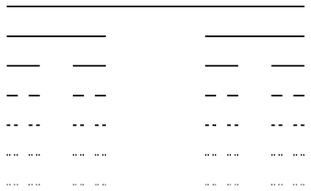
Figure 1: The finite iteration for constructing the triadic Cantor set.

The integral staircase function for the triadic Cantor set is defined as [12, 13].

$$S_{F}^{\alpha}(x)=\left\{\begin{array}[]{ll}\gamma^{\alpha}(F,a,b),&~{}\textmd{if}~{}x\geq a_{0},\\ -\gamma^{\alpha}(F,a,b),&~{}\textmd{othewise}.\end{array}\right.$$ (1)

where $\alpha$ is the $\gamma$-dimension of triadic Cantor set. In Figure 2 we plot the integral staircase function for triadic Cantor set.

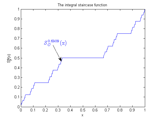
Figure 2: We plot the integral staircase function for triadic Cantor.

The definitions of $F^{\alpha}$-limit, $F^{\alpha}$-continuity and $F^{\alpha}$-integration are given in the ref. [12, 13]. The $F^{\alpha}$-differentiation is denoted by $D_{F}^{\alpha}$ and it is defined as

$$D_{F}^{\alpha}f(x)=\left\{\begin{array}[]{ll}F-\lim_{y\rightarrow x}\frac{f(y)-f(x)}{S_{F}^{\alpha}(y)-S_{F}^{\alpha}(x)},&\textmd{if}~{}~{}x\in F,\\ 0,&\textmd{otherwise,}\end{array}\right.$$ (2)

if the limit exists [12, 13].
Definition 1. The Gamma function with the fractal support is defined as

$$\Gamma_{F}^{\alpha}(x)=\int_{S_{F}^{\alpha}(0)}^{S_{F}^{\alpha}(\infty)}e^{-S_{F}^{\alpha}(t)}S_{F}^{\alpha}(t)^{S_{F}^{\alpha}(x)-1}d_{F}^{\alpha}t,$$ (3)

where

$$e^{-S_{F}^{\alpha}(t)}=F-\lim_{n\rightarrow\infty}(1-\frac{S_{F}^{\alpha}(t)}{n})^{n}.$$ (4)

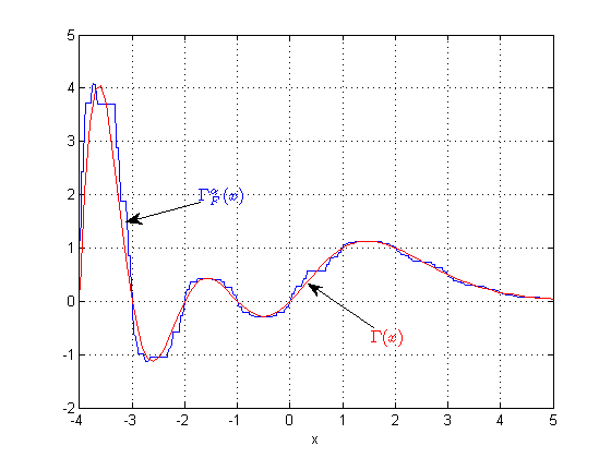
Figure 3: We sketch the fractal Gamma function which is compared with the standard case.

Definition 2. The fractal Beta function on the fractal set is defined as follows

$$B_{F}^{\alpha}(r,w)=\int_{0}^{1}S_{F}^{\alpha}(\zeta)^{r-1}(1-S_{F}^{\alpha}(\zeta))^{w-1}d_{F}^{\alpha}\zeta,$$ (5)

which is called two-parameter $(r,w)$ fractal integral, where $~{}\Re(r)>0$ and $\Re(w)>0$.
In the following we present some properties of fractal Beta function.
1) The fractal Beta function has a symmetry $B_{F}^{\alpha}(w,r)=B_{F}^{\alpha}(r,w)$. Since, we have

$$B_{F}^{\alpha}(r,w)=\int_{S_{F}^{\alpha}(0)}^{S_{F}^{\alpha}(1)}(S_{F}^{\alpha}(x))^{r-1}(1-S_{F}^{\alpha}(x))^{w-1}d_{F}^{\alpha}x,$$ (6)

using the transformation $S_{F}^{\alpha}(x)=1-S_{F}^{\alpha}(y)$, we conclude that

$$B_{F}^{\alpha}(r,w)=\int_{S_{F}^{\alpha}(0)}^{S_{F}^{\alpha}(1)}(1-S_{F}^{\alpha}(y))^{r-1}(S_{F}^{\alpha}(y))^{w-1}d_{F}^{\alpha}y=B_{F}^{\alpha}(w,r).$$ (7)

2) Using the transformation $S_{F}^{\alpha}(x)=\sin^{2}(S_{F}^{\alpha}(\theta))$, we get following form for the fractal the Beta function

$$B_{F}^{\alpha}(r,w)=\int_{S_{F}^{\alpha}(0)}^{S_{F}^{\alpha}(\pi/2)}\sin^{2}(S_{F}^{\alpha}(\theta))^{r-1}\cos^{2}(S_{F}^{\alpha}(\theta))^{w-1}(2\sin(S_{F}^{\alpha}(\theta))\cos(S_{F}^{\alpha}(\theta)))d_{F}^{\alpha}x,$$ (8)

$$=2\int_{S_{F}^{\alpha}(0)}^{S_{F}^{\alpha}(\pi/2)}\sin^{2r-1}(S_{F}^{\alpha}(\theta))\cos^{2w-1}(S_{F}^{\alpha}(\theta))d_{F}^{\alpha}x.$$ (9)

3) The Beta fractal function is related to the fractal Gamma function as

$$B_{F}^{\alpha}(r,w)=\frac{\Gamma_{F}^{\alpha}(r)\Gamma_{F}^{\alpha}(w)}{\Gamma_{F}^{\alpha}(r+w)}.$$ (10)

Proof: We have

$$\Gamma_{F}^{\alpha}(r)\Gamma_{F}^{\alpha}(w)=4\int_{S_{F}^{\alpha}(0)}^{S_{F}^{\alpha}(\infty)}(S_{F}^{\alpha}(x))^{2r-1}(S_{F}^{\alpha}(y))^{2w-1}e^{S_{F}^{\alpha}(x)^{2}+S_{F}^{\alpha}(y)^{2}}d_{F}^{\alpha}xd_{F}^{\alpha}y.$$ (11)

Transforming to polar coordinates $S_{F}^{\alpha}(x)=S_{F}^{\alpha}(\rho)\cos(S_{F}^{\alpha}(\phi)),~{}~{}~{}S_{F}^{\alpha}(x)=S_{F}^{\alpha}(\rho)\sin(S_{F}^{\alpha}(\phi))$ we obtain

$$\Gamma_{F}^{\alpha}(r)\Gamma_{F}^{\alpha}(w) =4\int_{S_{F}^{\alpha}(0)}^{S_{F}^{\alpha}(\infty)}(S_{F}^{\alpha}(\rho))^{2(r+w)-1}e^{-S_{F}^{\alpha}(\rho)^{2}}d_{F}^{\alpha}\rho\int_{S_{F}^{\alpha}(0)}^{S_{F}^{\alpha}(\pi/2)}\cos^{2r-1}(S_{F}^{\alpha}(\phi))\sin^{2w-1}(S_{F}^{\alpha}(\phi))d_{F}^{\alpha}\phi,$$

$$=B_{F}^{\alpha}(r,w)\Gamma_{F}^{\alpha}(r+w).$$ (12)

Thus, the proof is completed.

3 Non-local fractal derivative and integral

In this section, we define the non-local derivative for the functions with fractal support.
Definition 3. If $f(x)\in C_{F}^{\alpha}[a,b]$ ($\alpha$-order differentiable function on $[a,b]$) and $\beta>0$ then we have

$$_{a}\mathcal{I}_{x}^{\beta}f(x):=\frac{1}{\Gamma_{F}^{\alpha}(\beta)}\int_{S_{F}^{\alpha}(a)}^{S_{F}^{\alpha}(x)}\frac{f(t)}{(S_{F}^{\alpha}(x)-S_{F}^{\alpha}(t))^{\alpha-\beta}}d_{F}^{\alpha}t,~{}~{}~{}~{}S_{F}^{\alpha}(x)>S_{F}^{\alpha}(a),$$ (13)

where if $\beta=\alpha$ then we have fractal integral whose order is equal the dimension of the fractal, and

$$_{x}\mathcal{I}_{b}^{\beta}f(x):=\frac{1}{\Gamma_{F}^{\alpha}(\beta)}\int_{S_{F}^{\alpha}(x)}^{S_{F}^{\alpha}(b)}\frac{f(t)}{(S_{F}^{\alpha}(x)-S_{F}^{\alpha}(t))^{\alpha-\beta}}d_{F}^{\alpha}t,~{}~{}~{}~{}S_{F}^{\alpha}(x)<S_{F}^{\alpha}(b),$$ (14)

are called the analogous left sided and the right sided Riemann-Liouville fractal integral of order $\beta$.
Definition 4. Let $n-\alpha\leq\beta<n$, then analogous left and right Riemann-Liouville fractal derivative are defined as follows:

$${}_{a}\mathcal{D}_{x}^{\beta}f(x):=\frac{1}{\Gamma_{F}^{\alpha}(n-\beta)}(D_{F}^{\alpha})^{n}\int_{S_{F}^{\alpha}(a)}^{S_{F}^{\alpha}(x)}\frac{f(t)}{(S_{F}^{\alpha}(x)-S_{F}^{\alpha}(t))^{-n+\beta+\alpha}}d_{F}^{\alpha}t,$$ (15)

$${}_{x}\mathcal{D}_{b}^{\beta}f(x):=\frac{1}{\Gamma_{F}^{\alpha}(n-\beta)}(-D_{F}^{\alpha})^{n}\int_{S_{F}^{\alpha}(x)}^{S_{F}^{\alpha}(b)}\frac{f(t)}{(S_{F}^{\alpha}(t)-S_{F}^{\alpha}(x))^{-n+\beta+\alpha}}d_{F}^{\alpha}t.$$ (16)

Definition 5. Let $f(x)\in C^{\alpha n}[a,b]$, then the analogous left sided Caputo fractal derivative is defined by

$$_{a}^{C}\mathcal{D}_{x}^{\beta}f(x):=\frac{1}{\Gamma_{F}^{\alpha}(n-\beta)}\int_{S_{F}^{\alpha}(a)}^{S_{F}^{\alpha}(x)}(S_{F}^{\alpha}(x)-S_{F}^{\alpha}(t))^{n-\beta-\alpha}(D_{F}^{\alpha})^{n}f(t)d_{F}^{\alpha}t,~{}~{}~{}n=\max(0,-[-\beta]).$$ (17)

Also, the analogous right sided Caputo fractal derivative has the form

$${}_{x}^{C}\mathcal{D}_{b}^{\beta}f(x):=\frac{1}{\Gamma_{F}^{\alpha}(n-\beta)}\int_{S_{F}^{\alpha}(x)}^{S_{F}^{\alpha}(b)}(S_{F}^{\alpha}(t)-S_{F}^{\alpha}(x))^{n-\beta-\alpha}(-D_{F}^{\alpha})^{n}f(t)d_{F}^{\alpha}t.$$ (18)

Now, we give some important relations, namely

$$_{a}\mathcal{I}_{x}^{\beta}(S_{F}^{\alpha}(x)-S_{F}^{\alpha}(a))^{\eta}=\frac{\Gamma_{F}^{\alpha}(\eta+1)}{\Gamma_{F}^{\alpha}(\eta+\beta+1)}(S_{F}^{\alpha}(x)-S_{F}^{\alpha}(a))^{\eta+\beta},~{}~{}~{}\eta>-1.$$ (19)

Proof: Using the Eq. (13) we conclude

$$_{a}\mathcal{I}_{x}^{\beta}(S_{F}^{\alpha}(x)-S_{F}^{\alpha}(a))^{\eta}=\frac{1}{\Gamma_{F}^{\alpha}(\beta)}\int_{S_{F}^{\alpha}(a)}^{S_{F}^{\alpha}(x)}(S_{F}^{\alpha}(x)-S_{F}^{\alpha}(t))^{\beta-1}(S_{F}^{\alpha}(t)-S_{F}^{\alpha}(a))^{\eta}d_{F}^{\alpha}t.$$ (20)

Let us consider

$$S_{F}^{\alpha}(\xi)=\frac{S_{F}^{\alpha}(t)-S_{F}^{\alpha}(a)}{S_{F}^{\alpha}(x)-S_{F}^{\alpha}(a)},~{}~{}~{}~{}~{}~{}~{}~{}d_{F}^{\alpha}t=(S_{F}^{\alpha}(x)-S_{F}^{\alpha}(a))d_{F}^{\alpha}\xi.~{}~{}~{}~{}~{}$$ (21)

Therefore, $S_{F}^{\alpha}(\xi):S_{F}^{\alpha}(0)\rightarrow S_{F}^{\alpha}(1)$ while $S_{F}^{\alpha}(t):S_{F}^{\alpha}(a)\rightarrow S_{F}^{\alpha}(x)$. As a result we obtain

$$S_{F}^{\alpha}(x)-S_{F}^{\alpha}(t)=\frac{S_{F}^{\alpha}(1)-S_{F}^{\alpha}(\xi)}{S_{F}^{\alpha}(\xi)}(S_{F}^{\alpha}(t)-S_{F}^{\alpha}(0)).$$ (22)

Substituting Eqs. ( 21) and ( 22) in Eq. (20) we conclude that

$${}_{a}\mathcal{I}_{x}^{\beta}(S_{F}^{\alpha}(x)-S_{F}^{\alpha}(a))^{\eta}=\frac{1}{\Gamma_{F}^{\alpha}(\beta)}\int_{S_{F}^{\alpha}(0)}^{S_{F}^{\alpha}(1)}(1-S_{F}^{\alpha}(\xi))^{\beta-1}S_{F}^{\alpha}(\xi)^{1-\beta}(S_{F}^{\alpha}(t)-S_{F}^{\alpha}(a))^{\beta+\eta-1}(S_{F}^{\alpha}(x)-S_{F}^{\alpha}(a))d_{F}^{\alpha}\xi,$$

$$=\frac{1}{\Gamma_{F}^{\alpha}(\beta)}\int_{S_{F}^{\alpha}(0)}^{S_{F}^{\alpha}(1)}(1-S_{F}^{\alpha}(\xi))^{\beta-1}\left(\frac{S_{F}^{\alpha}(t)-S_{F}^{\alpha}(a)}{S_{F}^{\alpha}(x)-S_{F}^{\alpha}(a)}\right)^{1-\beta}(S_{F}^{\alpha}(t)-S_{F}^{\alpha}(a))^{\beta+\eta-1}(S_{F}^{\alpha}(x)-S_{F}^{\alpha}(a))d_{F}^{\alpha}\xi.$$ (23)

Then, we have

$$_{a}\mathcal{I}_{x}^{\beta}(S_{F}^{\alpha}(x)-S_{F}^{\alpha}(a))^{\eta}=\frac{(S_{F}^{\alpha}(x)-S_{F}^{\alpha}(a))^{\beta+\eta}}{\Gamma_{F}^{\alpha}(\beta)}\int_{S_{F}^{\alpha}(0)}^{S_{F}^{\alpha}(1)}(1-S_{F}^{\alpha}(\xi))^{\beta-1}(S_{F}^{\alpha}(\xi))^{\eta}d_{F}^{\alpha}\xi.$$ (24)

In view of Eq. (5) we derive

$$_{a}\mathcal{I}_{x}^{\beta}(S_{F}^{\alpha}(x)-S_{F}^{\alpha}(a))^{\eta}=\frac{(S_{F}^{\alpha}(x)-S_{F}^{\alpha}(a))^{\beta+\eta}}{\Gamma_{F}^{\alpha}(\beta)}B_{F}^{\alpha}(\beta,\eta+1).$$ (25)

Applying Eq. (10) we get

$$_{a}\mathcal{I}_{x}^{\beta}(S_{F}^{\alpha}(x)-S_{F}^{\alpha}(a))^{\eta} =\frac{(S_{F}^{\alpha}(x)-S_{F}^{\alpha}(a))^{\beta+\eta}}{\Gamma_{F}^{\alpha}(\beta)}\frac{\Gamma_{F}^{\alpha}(\beta)\Gamma_{F}^{\alpha}(\eta+1)}{\Gamma_{F}^{\alpha}(\beta+\eta+1)},$$

$$=\frac{\Gamma_{F}^{\alpha}(\eta+1)}{\Gamma_{F}^{\alpha}(\beta+\eta+1)}(S_{F}^{\alpha}(x)-S_{F}^{\alpha}(a))^{\beta+\eta}.$$ (26)

Now, we consider following formula

$$_{a}\mathcal{D}_{x}^{\beta}(S_{F}^{\alpha}(x)-S_{F}^{\alpha}(a))^{\eta}=\frac{\Gamma_{F}^{\alpha}(\eta+1)}{\Gamma_{F}^{\alpha}(\eta+1-\beta)}(S_{F}^{\alpha}(x)-S_{F}^{\alpha}(a))^{\eta-\beta}.$$ (27)

Proof: By rewriting the Eq. (27) we get

$$_{a}\mathcal{D}_{x}^{\beta}(S_{F}^{\alpha}(x)-S_{F}^{\alpha}(a))^{\eta}=(D_{F}^{\alpha})^{n}~{}_{a}\mathcal{I}_{x}^{n-\beta}(S_{F}^{\alpha}(x)-S_{F}^{\alpha}(a))^{\eta}.$$ (28)

Utilizing the Eq. (19) we conclude

$$_{a}\mathcal{D}_{x}^{\beta}(S_{F}^{\alpha}(x)-S_{F}^{\alpha}(a))^{\eta} =\frac{\Gamma_{F}^{\alpha}(\eta+1)}{\Gamma_{F}^{\alpha}(\eta+n-\beta+1)}(D_{F}^{\alpha})^{n}(S_{F}^{\alpha}(x)-S_{F}^{\alpha}(a))^{\eta+n-\beta},$$ (29)

$$=\frac{\Gamma_{F}^{\alpha}(\eta+1)}{\Gamma_{F}^{\alpha}(\eta-\beta+1)}(D_{F}^{\alpha})^{n}(S_{F}^{\alpha}(x)-S_{F}^{\alpha}(a))^{\eta-\beta},~{}~{}~{}\eta>-1.$$ (30)

Now, we write some important composition relations, namely

$$_{a}\mathcal{I}_{x}^{\beta}~{}_{a}\mathcal{D}_{x}^{\beta}f(x)=f(x)-\sum_{j=1}^{n}\frac{(_{a}\mathcal{D}_{x}^{\beta-j}f(x))|_{(S_{F}^{\alpha}(a))}}{\Gamma_{F}^{\alpha}(\beta+1-j)}(S_{F}^{\alpha}(x)-S_{F}^{\alpha}(a))^{\beta-j}.$$ (31)

Proof: Using the definitions we get

$$_{a}\mathcal{I}_{x}^{\beta}~{}_{a}\mathcal{D}_{x}^{\beta}f(x) =\frac{1}{\Gamma_{F}^{\alpha}(\beta)}\int_{S_{F}^{\alpha}(a)}^{S_{F}^{\alpha}(x)}(S_{F}^{\alpha}(x)-S_{F}^{\alpha}(t))^{\beta-1}\mathcal{D}_{x}^{\beta}f(t)d_{F}^{\alpha}t$$ (32)

$$=\frac{1}{\Gamma_{F}^{\alpha}(\beta+1)}D_{F}^{\alpha}\int_{S_{F}^{\alpha}(a)}^{S_{F}^{\alpha}(x)}(S_{F}^{\alpha}(x)-S_{F}^{\alpha}(t))^{\beta}(D_{F}^{\alpha})^{n}~{}_{a}\mathcal{I}_{x}^{n-\beta}f(t)d_{F}^{\alpha}tf(t)d_{F}^{\alpha}t.$$ (33)

Applying, n-times integration by part it leads to

$$_{a}\mathcal{I}_{x}^{\beta}~{}_{a}\mathcal{D}_{x}^{\beta}f(x) =D_{F}^{\alpha}~{}_{a}\mathcal{I}_{x}^{\beta+1-n}(_{a}\mathcal{I}_{x}^{n-\beta}f(x))-\sum_{k=1}^{n}\frac{(D_{F}^{\alpha})^{n-k}~{}_{a}\mathcal{D}_{x}^{\beta-n}f(x)|_{S_{F}^{\alpha}(a)}}{\Gamma_{F}^{\alpha}(\beta-k+1)}(S_{F}^{\alpha}(x)-S_{F}^{\alpha}(a))^{\beta-k},$$

$$=f(x)-\sum_{k=1}^{n}~{}\frac{{}_{a}\mathcal{D}_{x}^{\beta-k}f(x)|_{S_{F}^{\alpha}(a)}}{\Gamma_{F}^{\alpha}(\beta-k+1)}(S_{F}^{\alpha}(x)-S_{F}^{\alpha}(a))^{\beta-k}.$$ (34)

The similar proof works for the following formulas

$${}_{x}\mathcal{I}_{b}^{\beta}~{}_{x}\mathcal{D}_{b}^{\beta}f(x)=f(x)-\sum_{j=1}^{n}\frac{(_{x}\mathcal{D}_{b}^{\beta-j}f(x))|_{(S_{F}^{\alpha}(b))}}{\Gamma_{F}^{\alpha}(\beta+1-j)}(S_{F}^{\alpha}(b)-S_{F}^{\alpha}(x))^{\beta-j},$$ (35)

$${}_{a}\mathcal{I}_{x}^{\beta}~{}_{a}^{C}\mathcal{D}_{x}^{\beta}f(x)=f(x)-\sum_{j=1}^{n}\frac{((D_{F}^{\alpha})^{j}f(x))|_{(S_{F}^{\alpha}(a))}}{\Gamma_{F}^{\alpha}(j+1)}(S_{F}^{\alpha}(x)-S_{F}^{\alpha}(a))^{j},$$ (36)

$${}_{x}\mathcal{I}_{b}^{\beta}~{}_{x}^{C}\mathcal{D}_{b}^{\beta}f(x)=f(x)-\sum_{j=1}^{n}\frac{((D_{F}^{\alpha})^{j}f(x))|_{(S_{F}^{\alpha}(b))}}{\Gamma_{F}^{\alpha}(j+1)}(S_{F}^{\alpha}(b)-S_{F}^{\alpha}(x))^{j}.$$ (37)

In figures 4 and 5 we compared the non-local standard derivative versus non-local fractal derivative and the generalized fractal integral.

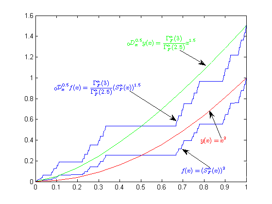
Figure 4: We plot $y(x)=x^{2}$ and $f(x)=S_{F}^{\alpha}(x)^{2}$ and their non-local derivative ${}_{0}D_{x}^{0.5}y(x)$ and ${}_{0}\mathcal{D}_{x}^{0.5}f(x)$, respectively.

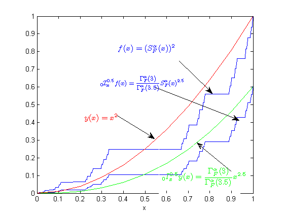
Figure 5: We show the graph of $g(x)=x^{2}$ and $f(x)=S_{F}^{\alpha}(x)^{2}$ and their non-local integral ${}_{0}I_{x}^{0.5}g(x)$ and ${}_{0}\mathcal{I}_{x}^{0.5}f(x)$, respectively.

4 Generalized functions in the non-local calculus on the fractal subset of real-line

In this section, we suggest the mathematical tools for solving the non-local fractal differential equations.

4.1 Gamma function on fractal subset of real line

Now, we define the Gamma function for the fractal calculus that will be used in non-local calculus on fractals.

4.2 Mittag-Leffler function on fractal subset of real-line

It is well known that the exponential function has important role in the theory of standard differential equation. The generalized exponential function is called the Mittag-Leffer function and plays an important role for fractional differential equations [1].
Definition 6. The generalized two parameter $\eta,\nu$ Mittag-Liffler function on fractal $F$ with $\alpha$-dimension is defined as

$$E_{F,\eta,\nu}^{\alpha}(x)=\sum_{k=0}^{\infty}\frac{S_{F}^{\alpha}(x)^{k}}{\Gamma_{F}^{\alpha}(\eta k+\nu)},~{}~{}~{}\eta>0,~{}~{}\nu\in\Re.$$ (38)

In the special case we have the following results, namely

$$E_{F,1,1}^{\alpha}(x) =e^{S_{F}^{\alpha}(x)},$$ (39)

$$E_{F,1,2}^{\alpha}(x) =\frac{e^{S_{F}^{\alpha}(x)-1}}{S_{F}^{\alpha}(x)},$$ (40)

$$E_{F,2,1}^{\alpha}(x) =\cosh(S_{F}^{\alpha}(x)),$$ (41)

$$E_{F,2,2}^{\alpha}(x) =\frac{\sinh(S_{F}^{\alpha}(x))}{S_{F}^{\alpha}(x)}.$$ (42)

4.3 Non-local Laplace transformation on fractal subset of real-line

The Laplace transformation is a very useful tool for solving standard linear differential equation with constant coefficients. The generalized Laplace transformation is applied to solve the fractional differential equations. Thus, in this section, we generalized the Laplace transformation for the function with fractal support which is utilized to solve the non-local differential equation on the fractal set [1].
Definition 7. Laplace transformation for the function $f(x)$ is denoted by $F(s)$ and it is defined as

$$\mathcal{F}_{F}^{\alpha}(S_{F}^{\alpha}(s))=\mathcal{L}_{F}^{\alpha}[f(x)]=\int_{S_{F}^{\alpha}(0)}^{S_{F}^{\alpha}(\infty)}f(x)e^{-S_{F}^{\alpha}(s)S_{F}^{\alpha}(x)}d_{F}^{\alpha}x.$$ (43)

Now, we give the fractal Laplace transformation of some functions. If we define the fractal convolution of two function $f(x)$ and $g(x)$ as follows:

$$f(x)*g(x)=\int_{S_{F}^{\alpha}(0)}^{S_{F}^{\alpha}(x)}f(S_{F}^{\alpha}(x)-S_{F}^{\alpha}(\tau))g(S_{F}^{\alpha}(\tau))d_{F}^{\alpha}\tau,$$ (44)

the fractal Laplace transformation of power function of $S_{F}^{\alpha}(x)$ is

$$\mathcal{L}_{F}^{\alpha}[S_{F}^{\alpha}(x)]\int_{S_{F}^{\alpha}(0)}^{S_{F}^{\alpha}(\infty)}S_{F}^{\alpha}(x)^{\beta}e^{-S_{F}^{\alpha}(s){S_{F}^{\alpha}(x)}}d_{F}^{\alpha}x=\frac{\Gamma_{F}^{\alpha}(1+\beta)}{s^{\beta+1}}.$$ (45)

Lemma: The Laplace transformation of the non-local fractal Riemann-Liouville integral is given by

$$\mathcal{L}_{F}^{\alpha}[_{0}\mathcal{I}_{x}^{\beta}f(x)]=\frac{\mathcal{F}_{F}^{\alpha}(S_{F}^{\alpha}(s))}{S_{F}^{\alpha}(s)^{\beta}}.$$ (46)

Proof: The Laplace transform of the fractal Riemann-Liouville integral is

$$\mathcal{L}_{F}^{\alpha}[_{0}\mathcal{I}_{x}^{\beta}f(x)]=\mathcal{L}_{F}^{\alpha}\left[\frac{1}{\Gamma_{F}^{\alpha}(\beta)}\int_{S_{F}^{\alpha}(0)}^{S_{F}^{\alpha}(x)}\frac{f(t)}{(S_{F}^{\alpha}(x)-S_{F}^{\alpha}(t))^{\alpha-\beta}}d_{F}^{\alpha}t\right].$$ (47)

Using the Eqs.(44) and (45) we arrive at

$$\mathcal{L}_{F}^{\alpha}[_{0}\mathcal{I}_{x}^{\beta}f(x)] =\frac{1}{\Gamma_{F}^{\alpha}(\beta)}\mathcal{F}_{F}^{\alpha}(S_{F}^{\alpha}(s))\mathcal{L}_{F}^{\alpha}[S_{F}^{\alpha}(x)^{\beta-1}],$$

$$=\frac{1}{\Gamma_{F}^{\alpha}(\beta)}\mathcal{F}_{F}^{\alpha}(S_{F}^{\alpha}(s))\frac{\Gamma_{F}^{\alpha}(\beta)}{S_{F}^{\alpha}(s)^{\beta}},$$

$$=\frac{\mathcal{F}_{F}^{\alpha}(S_{F}^{\alpha}(s))}{S_{F}^{\alpha}(s)^{\beta}}.$$ (48)

The fractal Laplace transform of the non-local fractal Riemann-Liouville derivative of order $\beta\in[0,1)$ is given by

$$\mathcal{L}_{F}^{\alpha}\{_{0}\mathcal{D}_{x}^{\beta}f(x),x,s\}=S_{F}^{\alpha}(s)^{\beta}\mathcal{F}_{F}^{\alpha}(s)-\sum_{k=1}^{n}S_{F}^{\alpha}(s)^{n-k}~{}_{0}\mathcal{D}_{x}^{\beta-n+k-1}f(x)|_{S_{F}^{\alpha}(0)},$$ (49)

where $n=[\beta]+1$. The fractal Laplace transform of the non-local fractal Caputo derivative of order $\beta\in[0,1)$ is given by

$$\mathcal{L}_{F}^{\alpha}\{_{0}^{C}\mathcal{D}_{x}^{\beta}f(x),x,s\}=(S_{F}^{\alpha}(s))^{\beta}\mathcal{F}_{F}^{\alpha}(s)-\sum_{k=1}^{n}S_{F}^{\alpha}(s)^{\beta-k}~{}_{0}\mathcal{D}_{x}^{k-1}f(x)|_{S_{F}^{\alpha}(0)}.$$ (50)

where $n=\max(0,-[-\beta])$.

5 Non-local fractal differential equations

In this section, we solve some illustrative examples.

Example 1. Consider the following linear fractal equation

$$_{0}^{C}\mathcal{D}_{x}^{\frac{1}{2}}y(x)=2,$$ (51)

with the initial condition

$$D_{F}^{\alpha}y(x)|_{S_{F}^{\alpha}(0)=0}=1,$$ (52)

where $\alpha=0.6309$ is Cantor set dimension. By applying ${}_{0}\mathcal{I}_{x}^{\frac{1}{2}}$ on the both sides of the Eq. (52) we obtain

$$y(x)=\frac{1}{\Gamma_{F}^{\alpha}(1+\frac{1}{2})}S_{F}^{\alpha}(x)+\frac{2}{\Gamma_{F}^{\alpha}(1-\frac{1}{2})}S_{F}^{\alpha}(x)^{-\frac{1}{2}}.$$ (53)

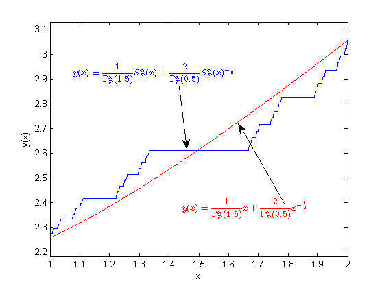
Figure 6: We present the solution of Eq. (51) on the real-line and Cantor set.

Example 2. Consider a linear fractal differential equation

$$_{0}^{C}\mathcal{D}_{x}^{\frac{1}{2}}y(x)=1-S_{F}^{\alpha}(x),~{}~{}~{}~{}S_{F}^{\alpha}(x)\geq 1,$$ (54)

with initial condition as

$$D_{F}^{\alpha}y(x)|_{S_{F}^{\alpha}(1)}=0.$$ (55)

By applying ${}_{0}\mathcal{I}_{x}^{\frac{1}{2}}$ on the both sides of the Eq. (55) we arrive at

$$y(x)=-\frac{\Gamma_{F}^{\alpha}(2)}{\Gamma_{F}^{\alpha}(2+\frac{1}{2})}(S_{F}^{\alpha}(x)-1)^{1+\frac{1}{2}},~{}~{}~{}S_{F}^{\alpha}(x)\geq 1.$$ (56)

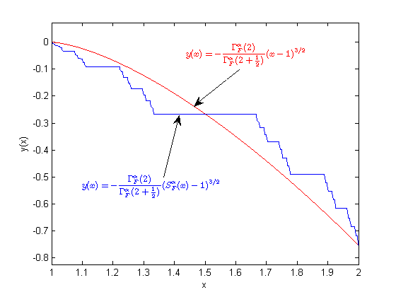
Figure 7: We give the graph of the solution of Eq. (54) on the real-line and Cantor set.

In Figures, 7 and 6 we plot the solutions of Eqs.(54) and (51), respectively.
Example 3. Consider a linear differential equation

$$_{0}\mathcal{D}_{x}^{\frac{1}{2}}y(x)=~{}y(x),~{}~{}~{}~{}~{}~{}~{}~{}~{}~{}$$ (57)

with the following initial condition, namely

$${}_{0}\mathcal{D}_{x}^{-\frac{1}{2}}y(x)|_{S_{F}^{\alpha}(0)}=1.$$ (58)

By inspection, the solution for the Eq. (57) becomes

$$y(x)=S_{F}^{\alpha}(x)^{-\frac{1}{2}}E_{F,1/2,1/2}^{\alpha}(-\sqrt{S_{F}^{\alpha}(x)}).$$ (59)

In Figure 8 we sketched the solution of Eq. (57) on the Cantor set and real-line.

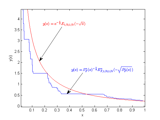
Figure 8: We plot the solution of Eq. (57) on the real-line and Cantor set.

Example 4. We examine the following non-local differential equation on a fractal subset of real-line, namely with the following initial condition

$${}_{0}\mathcal{D}_{F}^{\frac{4}{3}}y(x)-\lambda y(x)=(S_{F}^{\alpha}(x))^{2},~{}$$ (60)

$${}_{0}\mathcal{D}_{F}^{\frac{1}{3}}y(x)|_{S_{F}^{\alpha}(0)}=1,~{}~{}~{}~{}~{}~{}~{}~{}~{}~{}~{}~{}~{}~{}~{}_{0}\mathcal{D}_{F}^{\frac{-1}{6}}y(x)|_{S_{F}^{\alpha}(0)}=2.$$ (61)

For solving Eq. (60) we apply the fractal Laplace transformation on both side of it and we get

$$S_{F}^{\alpha}(s)^{\frac{4}{3}}\mathcal{F}_{F}^{\alpha}(s)-1-2(S_{F}^{\alpha}(s))^{\frac{1}{2}}-\lambda\mathcal{F}_{F}^{\alpha}(s)=\frac{2}{S_{F}^{\alpha}(s)^{3}}.$$ (62)

After some calculations we obtain

$$\mathcal{F}_{F}^{\alpha}(s)=\frac{1}{S_{F}^{\alpha}(s)^{\frac{4}{3}}-\lambda}+\frac{2S_{F}^{\alpha}(s)^{\frac{1}{2}}}{S_{F}^{\alpha}(s)^{\frac{4}{3}}-\lambda}+\frac{2S_{F}^{\alpha}(s)^{-3}}{S_{F}^{\alpha}(s)^{\frac{4}{3}}-\lambda}.$$ (63)

By computing the inverse fractal Laplace transform we conclude

$$y(x) =S_{F}^{\alpha}(x)^{\frac{4}{3}}E_{F,4/3,4/3}^{\alpha}(\lambda S_{F}^{\alpha}(x)^{\frac{4}{3}})+2S_{F}^{\alpha}(x)^{\frac{-1}{6}}E_{F,4/3,5/6}^{\alpha}(\lambda S_{F}^{\alpha}(x)^{\frac{4}{3}}$$

$$+2S_{F}^{\alpha}(x)^{\frac{10}{3}}E_{F,4/3,13/3}^{\alpha}(\lambda S_{F}^{\alpha}(x)^{\frac{4}{3}}.$$ (64)

Remark: The figures 6, 7, and 8 show that the solution of Eqs. (51), (54) and (57) leads to the standard non-local fractional cases when $\alpha=1$, respectively.

6 Conclusion

In this work, we defined new non-local derivatives on fractal sets. These new type of non-local derivatives can describe better the dynamics of complex systems which possess memory effect on a fractal set. Four illustrative examples were solved in detail. Finally, one can recover the standard non-local fractional cases when put $\alpha=1$.

All authors common finished the manuscript. All authors have read and approved the final manuscript.

The authors declare no conflict of interest.

References

• [1] Vladimir V. Uchaikin, Fractional Derivatives for Physicists and Engineers Vol. 1 Background and Theory. Vol 2. Application, Springer, Berlin, 2013.
• [2] D. Baleanu, K. Diethelm, E. Scalas, Juan J. Trujillo, Fractional Calculus Models and Numerical Methods. Ser. on Complexity, Nonlinearity and Chaos, World Scientific, 2012.
• [3] Stefan G. Samko, Anatoly A. Kilbas, Oleg I. Marichev, Fractional Integrals and Derivatives Theory and Applications, Gordon and Breach, New York, 1993.
• [4] I. Podlubny, Fractional Differential Equations. Academic, New York, 1999.
• [5] Skwara Urszula, et al., Applications of fractional calculus to epidemiological models, AIP Conference Proceedings-American Institute of Physics. 2012 , 1479 (1), 1339-1342.
• [6] Bruce J. West, M. Bologna, P. Grigolini, Physics of Fractal operators, New York, Springer, 2003
• [7] Alireza K. Golmankhaneh, Investigations in Dynamics: With Focus on Fractional Dynamics, LAP Lambert Academic Publishing, Saarbrucken, 2012.
• [8] D. Baleanu, Alireza K. Golmankhaneh, R. Nigmatullin, Ali K. Golmankhaneh, Fractional Newtonian mechanics, Cent. Eur. J. Phys. , 2010, 8(1), 120-125.
• [9] D. Baleanu, Alireza K. Golmankhaneh, Ali K. Golmankhaneh, Fractional nambu mechanics, Int. J. Theor. Phys., 2009, 48(4), 1044-1052.
• [10] D. Baleanu, Alireza K. Golmankhaneh, Ali K. Golmankhaneh, and Raoul R. Nigmatullin, Newtonian law with memory, Nonlinear Dyn., 2010, 60(1-2), 81-86.
• [11] Kiran M. Kolwankar, Anil D. Gangal, Fractional differentiability of nowhere differentiable functions and dimensions, Chaos: An Interdisciplinary J. Nonlinear Sci. , 1996, 6(4) , 505-513.
• [12] A. Parvate, Anil D. Gangal, Calculus on fractal subsets of real-line I: Formulation, Fractals, 2009, 17(01), 53-81.
• [13] A. Parvate, Anil D. Gangal, Calculus on fractal subsets of real-line II: Conjugacy with ordinary calculus, Fractals, 2011, 19(03), 271-290.
• [14] Benoit B. Mandelbrot, The Fractal Geometry of Nature, Freeman and Company, 1977.
• [15] K. Falconer, Techniques in Fractal Geometry, John Wiley and Sons, 1997.
• [16] J. Kigami, Analysis on fractals, Vol. 143, Cambridge University Press, 2001.
• [17] Xiao-Jun Yang, Advanced Local Fractional Calculus and Its Applications, World Science, New York, NY, USA 2012.
• [18] Alireza K. Golmankhaneh, Ali M. Yengejeh, D. Baleanu, On the fractional Hamilton and Lagrange mechanics, Int. J. Theor. Phys., 2012 51(9), 2909-2916.
• [19] Alireza K. Golmankhaneh, Ali K. Golmankhaneh, D. Baleanu, Lagrangian and Hamiltonian Mechanics on Fractals Subset of Real-Line, Int. J. Theor. Phys. 2013, 52(11), 4210-4217.
• [20] Alireza K. Golmankhaneh, Ali K. Golmankhaneh, D. Baleanu, About Maxwell’s equations on fractal subsets of $R^{3}$, Cent. Eur. J. Phys. 2013, 11 (6), 863-867.
• [21] Alireza K. Golmankhaneh, Ali K. Golmankhaneh, D. Baleanu, About Schröodinger Equation on Fractals Curves Imbedding in $R^{3}$ , Int. J. Theor. Phys., 2015, 54 (4) , 1275-1282.
• [22] Hari M. Srivastava, Alireza K. Golmankhaneh, D. Baleanu and Xiao-Jun Yang, Local fractional Sumudu transform with application to IVPs on Cantor sets, Abstr. Appl. Anal. 2014 Article ID 620529, 1-7.